CHAPTER 5 Data-Mining Predictions -...
32
Improving human-to-computer interaction through speech processing is just one area of computing that can benefit from enhanced computing. On the other side of the interface is the backend, which usually ties in to a database. It is here that enhanced computing can help users get the most from their data. Over the past ten years, there has been a dramatic increase in com- puter usage—and in the number of home users. Electronic commerce has resulted in the collection of vast amounts of customer and order informa- tion. In addition, most businesses have automated their processes and converted legacy data into electronic formats. Businesses large and small are now struggling with the question of what to do with all the electronic data they have collected. Data warehousing is a multi-billion-dollar industry that involves the collection, organization, and storage of large amounts of data. Data cubes—structures comprising one or more tables in a relational data- base—are built so that data can be examined through multiple dimen- sions. This allows databases containing millions of records and hundreds of attributes to be explored instantly. Data mining is the process of extracting meaningful information from large quantities of data. It involves uncovering patterns in the data and is often tied to data warehousing because it makes such large amounts of data usable. Data elements are grouped into distinct categories so that predictions can be made about other pieces of data. For example, a bank may wish to ascertain the characteristics that typify customers who pay back loans. Although this could be done with database queries, the bank would first have to know what customer attributes to query for. Data min- CHAPTER 5 Data-Mining Predictions 109
Transcript of CHAPTER 5 Data-Mining Predictions -...

Improving human-to-computer interaction through speech processing isjust one area of computing that can benefit from enhanced computing. Onthe other side of the interface is the backend, which usually ties in to adatabase. It is here that enhanced computing can help users get the mostfrom their data.
Over the past ten years, there has been a dramatic increase in com-puter usage—and in the number of home users. Electronic commerce hasresulted in the collection of vast amounts of customer and order informa-tion. In addition, most businesses have automated their processes andconverted legacy data into electronic formats. Businesses large and smallare now struggling with the question of what to do with all the electronicdata they have collected.
Data warehousing is a multi-billion-dollar industry that involves thecollection, organization, and storage of large amounts of data. Datacubes—structures comprising one or more tables in a relational data-base—are built so that data can be examined through multiple dimen-sions. This allows databases containing millions of records and hundredsof attributes to be explored instantly.
Data mining is the process of extracting meaningful information fromlarge quantities of data. It involves uncovering patterns in the data and isoften tied to data warehousing because it makes such large amounts ofdata usable. Data elements are grouped into distinct categories so thatpredictions can be made about other pieces of data. For example, a bankmay wish to ascertain the characteristics that typify customers who payback loans. Although this could be done with database queries, the bankwould first have to know what customer attributes to query for. Data min-
C H A P T E R 5
Data-Mining Predictions
109
ch05.qxd 3/7/05 10:38 AM Page 109

ing can be used to identify what those attributes are and then make pre-dictions about future customer behavior.
Data mining is a technique that has been around for several years. Un-fortunately, many of the original tools and techniques for mining data werecomplex and difficult for beginners to grasp. Microsoft and other softwaremakers have responded by creating easier-to-use data-mining tools. A 2004report titled “The Golden Vein” by the Economist.com states:
As the cost of storing data plummets and the power of analytic tools im-proves, there is little likelihood that enthusiasm for data mining, in all itsforms, will diminish.
This is the first of two chapters that will examine how a fictional re-tailer named Savings Mart was able to utilize Microsoft’s Analysis Ser-vices, included with Microsoft SQL Server, to improve operationalefficiencies and reduce costs. The present chapter will examine a stand-alone Windows program named LoadSampleData which is used to loadvalues into a database and generate random purchases for several of theretailer’s stores. A mining model will then be created based on shipmentsto each store. The mining model will be the first step toward revising theway Savings Mart procedurally handles product orders and shipments.
Chapter 6 will extend the predictions made in this chapter throughthe use of a Windows service designed to automate mining-model pro-cessing and the application of processing results. Finally, a modified ver-sion of the LoadSampleData program will be used to verify that SavingsMart was able to successfully lower its operating costs.
The chapter also includes a Microsoft case study which examines areal company that used Analysis Services to build a data-mining solution.In the case study, a leaser of technology equipment needed to predictwhen clients would return their leased equipment. By using Analysis Ser-vices, it was able to quickly build a data-mining solution that helped to re-duce costs and more accurately predict the value of assets.
Introducing Data Mining with SQL Server
Although SQL Server 7.0 offered Online Analytical Processing (OLAP) asOLAP Services, it was not until the release of SQL Server 2000 that data-mining algorithms were included. Analysis Services comes bundled withSQL Server as a separate install. It allows developers to build complex
110 Chapter 5 Data Mining Predictions
ch05.qxd 3/7/05 10:38 AM Page 110

OLAP cubes and then utilize two popular data-mining algorithms toprocess data within the cubes.
Of course, it is not necessary to build OLAP cubes in order to utilizedata-mining techniques. Analysis Services also allows mining models to bebuilt against one or more tables from a relational database. This is a bigdeparture from traditional data-mining methodologies. It means that userscan access data-mining predictions without the need for OLAP services.
Data mining involves the gathering of knowledge to facilitate betterdecision-making. It is meant to empower organizations to learn from theirexperiences—or in this case their historical data—in order to form proac-tive and successful business strategies. It does not replace decision-makers, but instead provides them with a useful and important tool.
The introduction of data-mining algorithms with SQL Server repre-sents an important step toward making data mining accessible to morecompanies. The built-in tools allow users to visually create mining modelsand then train those models with historical data from relational databases.
Data-Mining Algorithms
Data mining with Analysis Services is accomplished using one of two pop-ular mining algorithms—decision trees and clustering. These algorithmsare used to find meaningful patterns in a group of data and then makepredictions about the data. Table 5.1 lists the key terms related to datamining with Analysis Services.
Decision Trees
Decision trees are useful for predicting exact outcomes. Applying thedecision trees algorithm to a training dataset results in the formation of atree that allows the user to map a path to a successful outcome. At everynode along the tree, the user answers a question (or makes a “decision”),such as “years applicant has been at current job (0–1, 1–5, > 5 years).”
The decision trees algorithm would be useful for a bank that wants toascertain the characteristics of good customers. In this case, the predictedoutcome is whether or not the applicant represents a bad credit risk. Theoutcome of a decision tree may be a Yes/No result (applicant is/is not abad credit risk) or a list of numeric values, with each value assigned aprobability. We will see the latter form of outcome later in this chapter.
The training dataset consists of the historical data collected from pastloans. Attributes that affect credit risk might include the customer’s edu-cational level, the number of kids the customer has, or the total household
Introducing Data Mining with SQL Server 111
ch05.qxd 3/7/05 10:38 AM Page 111

112 Chapter 5 Data Mining Predictions
Term Definition
Case The data and relationships that represent a single objectyou wish to analyze. For example, a product and all its at-tributes, such as Product Name and Unit Price. It is notnecessarily equivalent to a single row in a relational table,because attributes can span multiple related tables. Theproduct case could include all the order detail records for asingle product.
Case Set Collection of related cases. This represents the way thedata is viewed and not necessarily the data itself. One caseset involving products could focus on the product, whereasanother may focus on the purchase detail for the sameproduct.
Clustering One of two popular algorithms used by Analysis Servicesto mine data. Clustering involves the classification of datainto distinct groups. As opposed to the other algorithm,decision trees, clustering does not require an outcomevariable.
Cubes Multidimensional data structures built from one or moretables in a relational database. Cubes can be the input for adata-mining model, but with Analysis Services the inputcould also be based on an actual relational table(s).
Decision Trees One of two popular algorithms used by Analysis Servicesto mine data. Decision trees involves the creation of atree that allows the user to map a path to a successfuloutcome.
Testing Dataset A portion of historical data that can be used to validate thepredictions of a trained mining model. The model will betrained using a training dataset that is representative of allhistorical data. By using a testing dataset, the developer canensure that the mining model was designed correctly andcan be trusted to make useful predictions.
Training Dataset A portion of historical data that is representative of allinput data. It is important that the training dataset repre-sent input variables in a way that is proportional to occur-rences in the entire dataset. In the case of Savings Mart,we would want the training dataset to include all the storesthat were open during the same time period so that no biasis unintentionally introduced.
Table 5.1 Key terms related to data mining with Analysis Services.
ch05.qxd 3/7/05 10:38 AM Page 112

income. Each split on the tree represents a decision that influences thefinal predicted variable. For example, a customer who graduated fromhigh school may be more likely to pay back the loan. The variable used inthe first split is considered the most significant factor. So if educationallevel is in the first split, it is the factor that most influences credit risk.
Clustering
Clustering is different from decision trees in that it involves groupingdata into meaningful clusters with no specific outcome. It goes through alooped process whereby it reevaluates each cluster against all the otherclusters looking for patterns in the data. This algorithm is useful when alarge database with hundreds of attributes is first evaluated. The cluster-ing process may uncover a relationship between data items that was neversuspected. In the case of the bank that wants to determine credit risk,clustering might be used to identify groups of similar customers. It couldreveal that certain customer attributes are more meaningful than origi-nally thought. The attributes identified in this process could then be usedto build a mining model with decision trees.
OLE DB for Data-Mining Specification
Analysis Services is based on the OLE DB for Data Mining (OLE DB forDM) specification. OLE DB for DM, an extension of OLE DB, was devel-oped by the Data Mining Group at Microsoft Research. It includes an Appli-cation Programming Interface (API) that exposes data-mining functionality.This allows third-party providers to implement their own data-mining algo-rithms. These algorithms can then be made available through the AnalysisServices Manager application when building new mining models.
TIP: Readers interested in learning more about the OLE DB for Data MiningSpecification can download documentation from the Microsoft Web site athttp://www.microsoft.com/downloads/details.aspx?FamilyID=01005f92-dba1-4fa4-8ba0-af6a19d30217&displaylang=en.
Savings Mart
Savings Mart is a fictitious discount retailer operating in a single Americanstate. It has been in business since 2001 and hopes to open new stores byachieving greater operational efficiencies. Since its inception, Savings
Savings Mart 113
ch05.qxd 3/7/05 10:38 AM Page 113

Mart has relied on a system of adjusting product inventory thresholds todetermine when shipments will be made to stores. Every time a product ispurchased, the quantity for that product and store is updated. When thequantity dips below the minimum threshold allowed for that product andstore, an order is automatically generated and a shipment is made threedays later.
Although this process seemed like a good way to ensure that the storeswere well stocked, it resulted in shipments being made to each store almostevery day. This resulted in high overhead costs for each store. Managementnow wishes to replace the order/shipment strategy with a system designedto predict shipment dates rather than rely on adjustable thresholds.
A sample application presented in this chapter allows the reader tocreate a training dataset for Savings Mart based on randomly generatedpurchases. The reader can then step through the process of creating amining model based on the dataset.
Loading the Savings Mart Database
To execute the sample code with SQL Server, you will need to create adatabase using a script file available on the book’s Web site. The installa-tion steps are as follows:
1. Open SQL Server’s Query Analyzer and connect to the serverwhere you wish to install the database.
2. Click File and Open…3. From the Open Query File dialog, browse to location of the
InstallDB.sql file available on the book’s Web site. Once selected,click OK.
4. Click Query and Execute or hit F5.5. Once the script has completed executing, a new database named
SavingsMart will be visible in the drop-down box on the toolbar.
Figure 5.1 is a diagram of the SavingsMart database. The Productstable contains a record for every product available in the stores. Eachproduct is associated with a certain vendor and assigned to a producttype, such as beverage or medicine. A field named DiscontinuedDate willcontain either a null, meaning it is not discontinued, or the date that itshould no longer be available for order. Every product should have aUnitQuantity of one or greater, which indicates the number of itemspackaged with that product. The products UnitPrice represents the retail
114 Chapter 5 Data Mining Predictions
ch05.qxd 3/7/05 10:38 AM Page 114

Savings Mart 115
Figu
re 5
.1Th
e S
avin
gsM
art
data
base
. Th
e sa
mpl
e da
taba
se c
onta
ins
five
hund
red
prod
ucts
and
fiv
e st
ores
.S
tore
s ar
e st
ocke
d w
ith a
ll pr
oduc
ts a
ccor
ding
to
thre
shol
d va
lues
con
tain
ed in
the
Pro
duct
Thre
shol
dsta
ble.
Each
tim
e a
prod
uct
is o
rder
ed a
nd a
shi
pmen
t co
mpl
eted
, th
e qu
antit
y fie
ld in
Pro
duct
Qty
is u
pdat
ed.
ch05.qxd 3/7/05 10:38 AM Page 115

price before any discounts are applied. The UnitType and UnitAmountfields may or may not contain values, depending on the product. For in-stance, a bottled water product will have a UnitType of “oz” and a Unit-Amount of 16.4, indicating that it weighs 16.4 fluid ounces. It is not nec-essary to record the weight of a mop, so for this product these valueswould be null.
The Purchases table is written to every time a customer makes a sin-gle purchase. It records information common to all purchases, such aswhen the purchase took place, what store it was made in, and what em-ployee rang up the purchase. Purchases are made for products availablewithin a particular store. Availability is determined by examining theQuantity field in the table ProductQty. A purchase can include multipleproducts and more than one unit of each product. The ProductDetailtable is a child of products, and it contains a record for each product asso-ciated with a single purchase. If the product purchased is on sale duringthe time of purchase, then the discount percentage, specified in the Pro-ductDiscounts table is applied.
Once a product is sold beneath the minimum threshold allowed for thestore, as indicated by the ProductThresholds table, an order is automati-cally placed. The quantity for the order is based on the maximum amountfound in the ProductThresholds table. Each shipment is the direct result ofan order and is typically completed three days after the order is placed.
Populating the Database
Once the SavingsMart database is created, the next step is to populate thedatabase. Unlike the sample databases in Chapters 2 and 3, the Savings-Mart database needs to be populated with a large quantity of data. To fa-cilitate this process and provide a method for generating unique trainingdatasets, a sample data-loading application is included on the book’s Website at http:// www.awprofessional.com/title/0321246268. The sample Win-dows application, named LoadSampleData, will allow you to simulate ran-dom purchases as well as to initiate orders and shipments needed torestock products.
Utilizing the LoadSampleData program ensures that you are dealingwith a clean database. Very often, the most difficult and time-consumingpart of successful data mining involves cleaning the historical database toremove or replace records holding invalid values. Refer to the next sec-tion, “Cleaning the Database,” for more information about this.
116 Chapter 5 Data Mining Predictions
ch05.qxd 3/7/05 10:38 AM Page 116
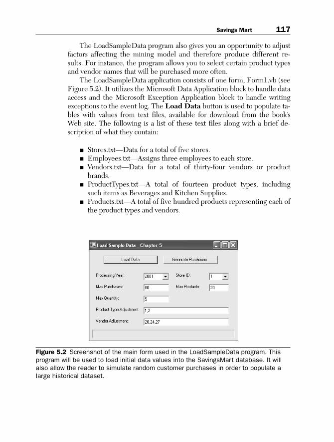
The LoadSampleData program also gives you an opportunity to adjustfactors affecting the mining model and therefore produce different re-sults. For instance, the program allows you to select certain product typesand vendor names that will be purchased more often.
The LoadSampleData application consists of one form, Form1.vb (seeFigure 5.2). It utilizes the Microsoft Data Application block to handle dataaccess and the Microsoft Exception Application block to handle writingexceptions to the event log. The Load Data button is used to populate ta-bles with values from text files, available for download from the book’sWeb site. The following is a list of these text files along with a brief de-scription of what they contain:
■ Stores.txt—Data for a total of five stores.■ Employees.txt—Assigns three employees to each store.■ Vendors.txt—Data for a total of thirty-four vendors or product
brands.■ ProductTypes.txt—A total of fourteen product types, including
such items as Beverages and Kitchen Supplies.■ Products.txt—A total of five hundred products representing each of
the product types and vendors.
Savings Mart 117
Figure 5.2 Screenshot of the main form used in the LoadSampleData program. Thisprogram will be used to load initial data values into the SavingsMart database. It willalso allow the reader to simulate random customer purchases in order to populate alarge historical dataset.
ch05.qxd 3/7/05 10:38 AM Page 117

The LoadData routine is also used to populate the ProductThresh-olds table with set values for minimum and maximum threshold amounts.The minimum field represents the minimum quantity of product thatshould be available in a certain store. The maximum field is the quantitythat will be ordered for that store when the minimum threshold is bro-ken. Initially, the minimum and maximum values will be set at ten andtwo hundred respectively. This will be the case for each product and eachstore, resulting in a total of twenty-five hundred records (500 products ×5 stores = 2500 records).
Finally, the LoadData routine will generate orders and shipments foreach of the five stores. The initial orders will stock the stores with themaximum threshold for all five hundred products. The shipment date willoccur three days after the order date to ensure that all stores are fullystocked on the first day of the year.
To begin loading data, execute the following steps:
1. Copy the contents of the LoadSampleData directory, available fordownload from the book’s Web site, to a location accessible byyour development machine. Note the location because it will beused to set the sPath variable in step 4.
2. Open the LoadSampleData project file with Visual Studio .NET.
3. From Solution Explorer, right-click Form1 and select ViewCode.
4. The top of the form contains two variables that will be unique toyour installation. Ensure that the sConn and sPath variables areset correctly. sConn is a string variable containing the connectionstring used to connect to the SavingsMart database on SQL Server. sPath is a string variable containing the file path to the text files.The text files reside in a subdirectory name TextFiles. This subdi-rectory is located inside the LoadSampleData directory (createdin step 1).
5. Execute the application by selecting Start from the DebugMenu. Figure 5.2 is a screenshot of form1.
6. To begin, click the Load Data button and ensure that the mes-sage box “Initial Data Load is complete” appears. Note that theform contains several combo and textboxes that will determinewhat and how data is loaded.
118 Chapter 5 Data Mining Predictions
ch05.qxd 3/7/05 10:38 AM Page 118
TIP: If you do not wish to load the database utilizing the sample applicationprovided, you can instead attach the database file supplied on the book’sWeb site. To attach the file, execute the following steps:
1. Copy the SavingsMart.mdf and SavingsMart.ldf files from thebook’s Web site to a local directory on the server where MicrosoftSQL Server is installed.
2. Open SQL Server’s Enterprise Manager.3. Right-click the Databases node and click All Tasks… and Attach
Database.4. From the Attach Database dialog, browse to the directory where you
copied the database files in step 1 and select the SavingsMart.mdffile. Click OK.
5. Click OK to attach the database.6. To see the newly added database, you will need to click Action and
Refresh.
The next step is to generate purchases for each of the five stores. Datamining is most effective in dealing with large datasets. Therefore, theGeneratePurchases routine, seen as follows, will insert approximately100,000 records in the PurchaseDetail table for each store and calendaryear. Purchases are generated for one store—one year at a time.
'Maximum # of purchases per day
Dim nMaxPurchases As Int16 = txtMaxPurchases.Text
'Maximum # of products per purchase
Dim nMaxProducts As Int16 = txtMaxProducts.Text
'Maximum value of quantity per product
Dim nMaxQuantity As Int16 = txtMaxQuantity.Text
Dim sYear As String = cboYear.Text
Dim nStoreID As Int16 = cboStoreID.Text
'These are the Product Types in which there is an
'increased chance of product selection
'The default of 1,2 represents snack foods and beverages
Dim sProductTypeAdj As String = txtProductTypeAdj.Text
'These are the Vendors in which there is an increased
'chance of product selection
'The default of 20,24,27 represents Kamp, Notch, and PNuts as Vendors
Dim sVendorAdj As String = txtVendorAdj.Text
Savings Mart 119
ch05.qxd 3/7/05 10:38 AM Page 119

ProgressBar1.Minimum = 1
ProgressBar1.Maximum = 366
Try
Dim params(2) As SqlParameter
params(0) = New _
SqlParameter("@ID", SqlDbType.Int)
params(1) = New _
SqlParameter("@ProdTypeAdj", SqlDbType.VarChar, 50)
params(2) = New _
SqlParameter("@VendorAdj", SqlDbType.VarChar, 50)
params(0).Value = nStoreID
params(1).Value = sProductTypeAdj
params(2).Value = sVendorAdj
Dim ds As DataSet = _
SqlHelper.ExecuteDataset(sConn, _
CommandType.StoredProcedure, "GetProductIDS", params)
Dim i As Int16 = 1
Dim dtDate As DateTime
dtDate = Convert.ToDateTime("01/01/" + sYear)
'Loop through everyday of the year
'We assume the store is open every day
Randomize()
Do Until i = 366
'First thing is check to see if orders needs to
'be fulfilled for this day and store
'We assume that all orders are shipped 3 days
'after the orderdate in one shipment
Dim params1(1) As SqlParameter
params1(0) = New _
SqlParameter("@StoreID", SqlDbType.Int)
params1(1) = New _
SqlParameter("@Date", SqlDbType.SmallDateTime)
params1(0).Value = nStoreID
'order was placed 3 days ago
params1(1).Value = dtDate.AddDays(-3)
SqlHelper.ExecuteReader(sConn, _
CommandType.StoredProcedure, "InsertShipment", params1)
Dim x As Int16 = 1
'This will be the total number of purchases for this day
Dim nPurchases As Int16
nPurchases = CInt(Int((nMaxPurchases * Rnd()) + 1))
Do Until x = nPurchases + 1
120 Chapter 5 Data Mining Predictions
ch05.qxd 3/7/05 10:38 AM Page 120
Dim y As Int16 = 1
Dim nEmployeePos As Int16
nEmployeePos = CInt(Int((ds.Tables(1).Rows.Count * Rnd())))
Dim nEmployeeID As Integer = _
Convert.ToInt32(ds.Tables(1).Rows(nEmployeePos).Item(0))
Dim params2(2) As SqlParameter
params2(0) = New SqlParameter("@ID1", SqlDbType.Int)
params2(1) = New _
SqlParameter("@Date", SqlDbType.SmallDateTime)
params2(2) = New SqlParameter("@ID2", SqlDbType.Int)
params2(0).Value = nStoreID
params2(1).Value = dtDate
params2(2).Value = nEmployeeID
Dim nPurchaseID As Integer = _
SqlHelper.ExecuteScalar(sConn, _
CommandType.StoredProcedure, "InsertPurchase", params2)
'This is total number of products for this purchase
Dim nProducts As Int16 = _
CInt(Int((nMaxProducts * Rnd()) + 1))
Do Until y = nProducts + 1
'This is quantity for this purchase
Dim nQty As Int16 = _
CInt(Int((nMaxQuantity * Rnd()) + 1))
'This is the product for this detail record
Dim nProductPos As Int16 = _
CInt(Int((ds.Tables(0).Rows.Count * Rnd())))
Dim nProductID As Integer = _
Convert.ToInt32(ds.Tables(0).Rows(nProductPos).Item(0))
'Generate the detail record
Dim params3(4) As SqlParameter
params3(0) = New SqlParameter("@StoreID", SqlDbType.Int)
params3(1) = New _
SqlParameter("@ProductID", SqlDbType.Int)
params3(2) = New _
SqlParameter("@PurchaseID", SqlDbType.Int)
params3(3) = New SqlParameter("@Qty", SqlDbType.Int)
params3(4) = New _
SqlParameter("@Date", SqlDbType.SmallDateTime)
params3(0).Value = nStoreID
params3(1).Value = nProductID
params3(2).Value = nPurchaseID
params3(3).Value = nQty
params3(4).Value = dtDate
Savings Mart 121
ch05.qxd 3/7/05 10:38 AM Page 121

SqlHelper.ExecuteScalar(sConn, _
CommandType.StoredProcedure, _
"InsertPurchaseDetail", params3)
y += 1
Loop
x += 1
Loop
i += 1
ProgressBar1.Value = i
'Go to the next day
dtDate = dtDate.AddDays(1)
Loop
MessageBox.Show("Purchases for store " _
+ Convert.ToString(cboStoreID.Text) + _
" were generated successfully")
Catch ex As Exception
MessageBox.Show(ex.Message)
ExceptionManager.Publish(ex)
End Try
The amount of records is approximate because the routine utilizes arandom number generator to determine the number of purchases per dayalong with the number of products per purchase. The number of recordsalso varies depending on what input variables are chosen on form1.
The program utilizes default values specifying that purchases will begenerated for Store 1 in the year 2001. The GeneratePurchases routinecontains a main loop that will execute 365 times for each day of one calen-dar year. The variable max purchases defaults to 80 and is used to providethe maximum value for the random number generator when determininghow many purchases will be generated for a single day.
The variable max products determines the number of distinct prod-ucts that will be used for a single purchase. Max quantity is used to de-termine the quantity used in a single purchase detail record. By utilizingthe random number generator and then adjusting these values for eachstore that is processed, we can simulate random purchase activity. In thesection titled “Interpreting the Results,” we will examine the results ofone mining model. To ensure that your results are consistent with theexplanations in this section, use the values in Table 5.2 when loadingyour database.
122 Chapter 5 Data Mining Predictions
ch05.qxd 3/7/05 10:38 AM Page 122

Savings Mart 123
Value (only use the number values and Store Field Caption not the literal values in parentheses)
1 Processing Year 2001Max Purchases 80Max Products 20Max Quantity 5Product Type Adjustment 1, 2 (Snack Foods and Beverages)Vendor Adjustment 20, 24, 27 (Kamp, Notch, and Pnuts)
2 Processing Year 2001Max Purchases 60Max Products 12Max Quantity 7Product Type Adjustment 2, 6 (Beverages and Baking Goods)Vendor Adjustment 13, 18 (Gombers and Joe’s)
3 Processing Year 2001Max Purchases 70Max Products 12Max Quantity 7Product Type Adjustment 2 (Beverages)Vendor Adjustment 34 (Store Brand)
4 Processing Year 2001Max Purchases 100Max Products 5Max Quantity 2Product Type Adjustment (leave blank)Vendor Adjustment 34, 18 (Store Brand and Joe’s)
5 Processing Year 2001Max Purchases 50Max Products 15Max Quantity 8Product Type Adjustment 6 (Baking Goods)Vendor Adjustment 24, 27, 34 (Notch, Pnuts, and Store
Brand)
Table 5.2 Values to be used in the LoadSampleData application when generatingpurchases for all five stores.
ch05.qxd 3/7/05 10:38 AM Page 123
Of course, since we are using a random number generator, the pur-chases generated will represent all products equally well over the longrun. The Product Type Adjustment and Vendor Adjustment variables areintroduced because equal distribution of product purchases is not realis-tic. These variables contain a comma-delimited list of ProductTypeID andVendorID values. The stored procedure GetProductIDs uses these val-ues when returning the dataset of available ProductID’s. If a Product-TypeID is specified, then every product that relates to that product typewill be included in the list of available product id’s more than once. Thiswill increase the chances that the product will be selected for the Pur-chaseDetail record. The Vendor Adjustment works similarly in that foreach VendorID specified, all products assigned to that vendor will appearin the available product list more than once.
If you do not alter the values on form1, the GeneratePurchases rou-tine will take approximately twenty minutes to load data for each store andcalendar year. A progress bar is used to indicate the status of the data loadbecause the process is somewhat time-consuming.
TIP: Although it is not necessary to execute the GeneratePurchases routinefor each store and all three years, make sure to load at least one store forone calendar year before continuing. This will provide you with enough datato use for processing.
Once the data has loaded, you should see a dialog with the message“Purchases were generated successfully.”
If you do not receive the successful message and instead receive anerror message, you will first need to resolve the error. Then you will need todelete the database from SQL Server Enterprise Manager and repeat thesteps used to load data.
If you continue to receive an error, consider attaching the database perthe instructions in the previous tip.
124 Chapter 5 Data Mining Predictions
Case Study: ComputerFleet
ComputerFleet, (www.computerfleet.com.au), based in Sydney, Australia,leases technology equipment to companies in a number of different in-dustries and to government agencies. Its wide range of clients includessmall, medium, and large organizations.
Since it was necessary to store a large amount of data (twelve yearsworth), ComputerFleet was using a data warehouse built on top of Mi-
ch05.qxd 3/7/05 10:38 AM Page 124
Cleaning the Database
Cleaning the database is one of the most important tasks in successful datamining. Databases to be mined are often constructed from multiple datasources. These data sources often involve data that is prone to a variety oferrors that can destroy any chance you have of making useful predictions.Most everyone has heard or used the phrase “Garbage in, Garbage out.”This phrase applies more than ever to data mining.
Possible errors include records with impossible values or values thatfall outside the expected range. Also, records that include null valueswhere nulls will negatively impact the decision-making process. Most ofthese errors could be prevented with database restrictions or applicationcode, but this does not always happen. Since our sample database was arti-ficially created, we can be reasonably sure that these errors do not exist.
Savings Mart 125
crosoft SQL Server 2000. The company was already using analysis toolslike Microsoft Data Analyzer and Microsoft Excel to report on the data.
What ComputerFleet needed was a way to predict when its clientswould return leased equipment. Unfortunately, this does not always occuron the agreed lease-end date. Having this information would allow Com-puterFleet to better manage its equipment and save money. The companywould also be in a better position to value its assets.
ComputerFleet asked a consulting company named Angry Koala(www.angrykoala.com.au) and Microsoft Consulting Services to help it ob-tain this information. Within a few weeks the consultants had built a data-mining solution with Microsoft Analysis Services.
The data-mining solution uses such attributes as the type of industry,type of equipment, and whether the client is new as input variables to themining model. The predicted results are stored back in the data ware-house as the predicted asset-arrival time.
ComputerFleet was pleased not only because it was able to makevaluable predictions, but because it did not have to purchase any extraproprietary software to do so. Also, it was easy to integrate the data-mining solution with the existing data warehouse in Microsoft SQLServer 2000.
This is a real example of a large company that was able to quicklytake advantage of the built-in functionality of Microsoft SQL Server to de-crease its operational costs. For more information about ComputerFleetand this Microsoft case study, go to www.microsoft.com/resources/cas-estudies/casestudy.asp?CaseStudyID=14375.
ch05.qxd 3/7/05 10:38 AM Page 125
The following is a list of the errors that could have occurred if our data-base existed in the real world:
■ Store sale in which the ending data occurs before the startingdate.
■ A purchase handled by a store employee before their hire date orfor a store they were not assigned to.
■ An order made for a product that was discontinued before theorder date.
■ A shipment or order date that is invalid or outside the days of oper-ation for the concerned store.
■ A negative quantity in either PurchaseDetail, OrderDetail, Ship-mentDetail, or ProductQty.
■ A product not associated with a vendor or a purchase with no pur-chase date and quantity.
■ A maximum amount that is greater than the minimum.
The methods used to clean a database can vary. Often, values can becorrected with a few update queries made in Query Analyzer. The hard-est part is determining what the correct values should be. More thanlikely, outside help will be needed from people intimately familiar with thedata, such as a store manager.
Creating Views
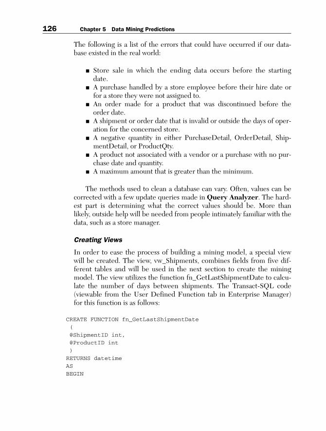
In order to ease the process of building a mining model, a special viewwill be created. The view, vw_Shipments, combines fields from five dif-ferent tables and will be used in the next section to create the miningmodel. The view utilizes the function fn_GetLastShipmentDate to calcu-late the number of days between shipments. The Transact-SQL code(viewable from the User Defined Function tab in Enterprise Manager)for this function is as follows:
CREATE FUNCTION fn_GetLastShipmentDate
(
@ShipmentID int,
@ProductID int
)
RETURNS datetime
AS
BEGIN
126 Chapter 5 Data Mining Predictions
ch05.qxd 3/7/05 10:38 AM Page 126

DECLARE @ShippedDate smalldatetime, @TShipmentID int, @ret
smalldatetime
DECLARE cursor1 CURSOR SCROLL
FOR select shippeddate, s.shipmentid from shipments s
left join shipmentdetails sd on s.shipmentid = sd.shipmentid
where s.storeid IN (SELECT StoreID FROM Shipments
WHERE shipmentid = @Shipmentid)
AND sd.productid = @ProductID
ORDER BY shippeddate
OPEN cursor1
FETCH NEXT FROM cursor1 INTO @ShippedDate, @TShipmentID
WHILE @@FETCH_STATUS = 0
BEGIN
IF @ShipmentID = @TShipmentID
BEGIN
FETCH PRIOR FROM cursor1 INTO @ShippedDate, @TShipmentID
SET @ret = @ShippedDate
GOTO Close_Cursor
END
FETCH NEXT FROM cursor1 INTO @ShippedDate, @TShipmentID
END
Close_Cursor:
CLOSE cursor1
DEALLOCATE cursor1
RETURN(@ret)
END
The function accepts @ShipmentID and @ProductID as input vari-ables. It then opens a scrollable cursor (similar to an ADO resultset) basedon the following SQL statement:
SELECT shippeddate, s.shipmentid FROM shipments s
LEFT JOIN shipmentdetails sd ON s.shipmentid = sd.shipmentid
WHERE s.storeid IN (SELECT StoreID FROM Shipments
WHERE shipmentid = @Shipmentid)
AND sd.productid = @ProductID
ORDER BY shippeddate
The function loops through the cursor results until it locates theShipmentID supplied as an input variable. Once located, it moves to the
Savings Mart 127
ch05.qxd 3/7/05 10:38 AM Page 127

preceding record and returns that shipment date. This shipment date isused as the first variable for the built-in SQL function DATEDIFF. Theresulting variable, DaysSinceLastShipped, will be an important columnfor the Analyze Shipments mining model.
Working with Mining Models
Building a Mining Model
Now that the database has been created and populated, the next step isto create a mining model. Mining models can be created with the Min-ing Model Editor in Analysis Manager or programmatically with De-cision Support Objects (DSO). Using DSO to create mining models isuseful when you need to programmatically automate the mining-modelprocess. For the most part, you will use Analysis Manager to create min-ing models.
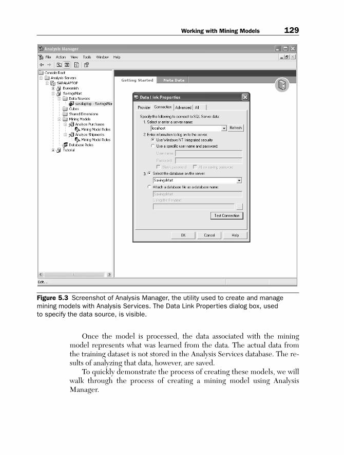
Analysis Manager (see Figure 5.3) allows you to create and managedatabases used by Analysis Services. A database node in Analysis Managerdoes not represent the physical storage of a large database. Instead, it rep-resents the database that Analysis Services will use to hold the mining-model definitions and the results of processing these mining models. Itwill, however, reference a physical data source.
Each database in Analysis Manager is associated with one or moredata sources. These data sources can be either relational databases or datawarehouses. Data sources are created by right-clicking the Data Sourcesnode and selecting New Data Source. From the Data Link Propertiesdialog, a data provider is selected along with the connection information.Analysis Services supports SQL Server, Access, and Oracle databases asdata sources.
Mining models are the blueprint for how the data should be analyzedor processed. Each model represents a case set, or a set of cases (see Table5.1). The mining-model object stores the information necessary to processthe model—for instance, what queries are needed to get the data fields,what data fields are input columns or predictable columns, and what rela-tionship each column has with other columns. Input columns are attrib-utes whose values will be used to generate results for the predictablecolumns. In some cases, the attribute may serve both as an input columnand a predictable column.
128 Chapter 5 Data Mining Predictions
ch05.qxd 3/7/05 10:38 AM Page 128
Once the model is processed, the data associated with the miningmodel represents what was learned from the data. The actual data fromthe training dataset is not stored in the Analysis Services database. The re-sults of analyzing that data, however, are saved.
To quickly demonstrate the process of creating these models, we willwalk through the process of creating a mining model using AnalysisManager.
Working with Mining Models 129
Figure 5.3 Screenshot of Analysis Manager, the utility used to create and manage mining models with Analysis Services. The Data Link Properties dialog box, used to specify the data source, is visible.
ch05.qxd 3/7/05 10:38 AM Page 129
TIP: If you have not already done so, you will need to install Analysis Ser-vices. It is available as a separate install with the SQL Server 2000 setup.Make sure that you install the latest Service Pack release for SQL Server. In-formation about how to obtain the latest SQL Server service pack can befound at http://support.microsoft.com/default.aspx?kbid=290211.
If you have problems connecting with Analysis Services, refer to the arti-cle by Alexander Chigrik titled, “Troubleshooting OLAP Problems” at http://databasejournal.com/features/mssql/article.php/1582491. This online ar-ticle, featured in the Database Journal, is a troubleshooting checklist forsolving common problems.
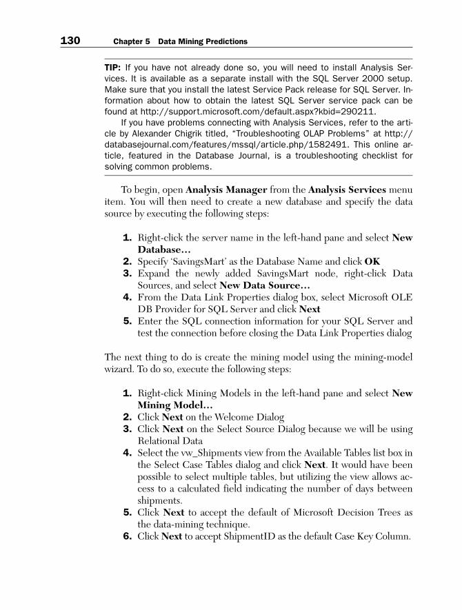
To begin, open Analysis Manager from the Analysis Services menuitem. You will then need to create a new database and specify the datasource by executing the following steps:
1. Right-click the server name in the left-hand pane and select NewDatabase…
2. Specify ‘SavingsMart’ as the Database Name and click OK3. Expand the newly added SavingsMart node, right-click Data
Sources, and select New Data Source…4. From the Data Link Properties dialog box, select Microsoft OLE
DB Provider for SQL Server and click Next5. Enter the SQL connection information for your SQL Server and
test the connection before closing the Data Link Properties dialog
The next thing to do is create the mining model using the mining-modelwizard. To do so, execute the following steps:
1. Right-click Mining Models in the left-hand pane and select NewMining Model…
2. Click Next on the Welcome Dialog3. Click Next on the Select Source Dialog because we will be using
Relational Data4. Select the vw_Shipments view from the Available Tables list box in
the Select Case Tables dialog and click Next. It would have beenpossible to select multiple tables, but utilizing the view allows ac-cess to a calculated field indicating the number of days betweenshipments.
5. Click Next to accept the default of Microsoft Decision Trees asthe data-mining technique.
6. Click Next to accept ShipmentID as the default Case Key Column.
130 Chapter 5 Data Mining Predictions
ch05.qxd 3/7/05 10:38 AM Page 130

7. Select the Finish the mining model in the editor checkbox andclick Next.
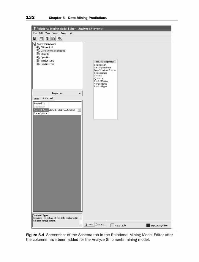
8. Name the model “Analyze Shipments” and click Finish.9. From the Relational Mining Model Editor, as seen in Figure 5.4,
click Insert and Column… and then select the column namedDaysSinceLastShipped. Once added, change the usage to Inputand Predictable (note that a diamond icon now appears next to thecolumn). Then go to the Advanced Properties and enter DIS-CRETIZED(CLUSTERS) as the content type.
NOTE: Choosing discretized as the content type allows a continuous variableto be grouped discretely instead. Continuous variables are usually numeric-based values that have an infinite range of possibilities. Since we need pre-dictable results, utilizing a discretization method allows for grouped results.DISCRETEIZED accepts two parameters, such as:
DISCRETIZED(<method>, <#buckets>)
where method could contain one of the following values:
EQUAL_AREAS—Divides into equal bucketsTHRESHOLDS—Uses inflection points to estimate bucket boundariesCLUSTERS—Uses a clustering algorithm to estimate bucketsAUTOMATIC (default)—Tries all algorithms and uses the first one that
suggests number buckets
10. Click Insert and Column… and then select the column namedStoreID. Once added, change the usage to Input and Predictable.
11. Click Insert and Column… and then select the column namedQuantity. Once added, change the usage to Predictable, and fromthe Advanced Properties tab, enter DISCRETIZED(CLUS-TERS) as the content type.
12. Click Insert and Column… and then select the column namedVendorName.
13. Click Insert and Column… and then select the column namedProductType.
14. Click Tools and Process Mining Model… Click OK when askedto save the mining model. Then click OK to start a full process ofthe mining model. This process will take several minutes to run ifyou loaded data for all five stores. When complete, the message“Processing Complete” will appear in green text.
Working with Mining Models 131
ch05.qxd 3/7/05 10:38 AM Page 131
132 Chapter 5 Data Mining Predictions
Figure 5.4 Screenshot of the Schema tab in the Relational Mining Model Editor afterthe columns have been added for the Analyze Shipments mining model.
ch05.qxd 3/7/05 10:38 AM Page 132

Training the Mining Model
Training the mining model is accomplished by processing the results of amining model using Analysis Manager. Alternatively, the same thing couldbe accomplished using a scripting language known as Data DefinitionLanguage (DDL) and a connection to the Analysis Server. We can seewhat DDL commands are used to train the model through the Processdialog box, as shown in Figure 5.5.
DDL is useful in cases when you want to programmatically process amining model. The language can be executed through a connection to theAnalysis Server. It is also useful for demonstrating how Analysis Managerprocesses a mining model.
A mining model is created using the CREATE MINING MODELsyntax. The syntax is similar to Transact SQL and should be instantly fa-miliar to SQL developers. The CREATE statement for this mining modelis as follows:
CREATE MINING MODEL [Analyze Shipments](
[Shipment Id] LONG KEY,
[Days Since Last Shipped] LONG DISCRETIZED(CLUSTERS) PREDICT,
[Store Id] LONG DISCRETE,
[Quantity] LONG DISCRETIZED(CLUSTERS) PREDICT_ONLY,
Working with Mining Models 133
Figure 5.5 Screenshot of the dialog that appears when full process is initiated for a mining model. Note the DDL syntax used to create the model and then train it bypopulating it with historical data.
ch05.qxd 3/7/05 10:38 AM Page 133

[Vendor Name] TEXT DISCRETE,
[Product Type] TEXT DISCRETE)
USING Microsoft_Decision_Trees
With the preceding statement, we are creating a new mining modelnamed Analyze Shipments. The model utilizes Shipment ID as the casekey. Days Since Last Shipped, and Quantity are each defined as pre-dictable columns, but Days Since Last Shipped also functions as an inputcolumn. The remaining columns, Store ID, Vendor Name, and ProductType, are input columns only. Mining-model columns are defined as ei-ther input, predictable, or input and predictable.
The process of training a model involves the insertion of data into themining model using the INSERT INTO syntax, as follows:
INSERT INTO [Analyze Shipments]
(SKIP,[Days Since Last Shipped], [Store Id], [Quantity],
[Vendor Name], [Product Type])
OPENROWSET('SQLOLEDB.1','Provider=SQLOLEDB.1;Integrated
Security=SSPI;Persist Security Info=False;Initial
Catalog=SavingsMart;Data Source=(local)',
'SELECT DISTINCT “dbo"."vw_Shipments"."ShipmentID"
AS "Shipment Id", "dbo"."vw_Shipments"."DaysSinceLastShipped"
AS "Days Since Last Shipped", "dbo"."vw_Shipments"."StoreID"
AS "Store Id", "dbo"."vw_Shipments"."Quantity" AS "Quantity",
"dbo"."vw_Shipments"."VendorName" AS "Vendor Name",
"dbo"."vw_Shipments"."ProductType" AS "Product Type"
FROM "dbo"."vw_Shipments"')
The mining model will not store the actual data, but will store the pre-diction results instead once the mining algorithm is processed. In the pre-ceding statement, the OPENROWSET keyword was used to specify thelocation of the physical data source.
Interpreting the Results
To examine the results from processing the model, select the Contenttab. Figure 5.6 is a screenshot of the content detail when analyzingDaysSinceLastShipped. This screen indicates that VendorName was themost significant factor affecting DaysSinceLastShipped. We know this be-cause it is the first split on the tree. For nodes that have additionalbranches, two lines will follow the node. To view the additional branches,double-click that node and the detail page will drill down to the next level.
134 Chapter 5 Data Mining Predictions
ch05.qxd 3/7/05 10:38 AM Page 134
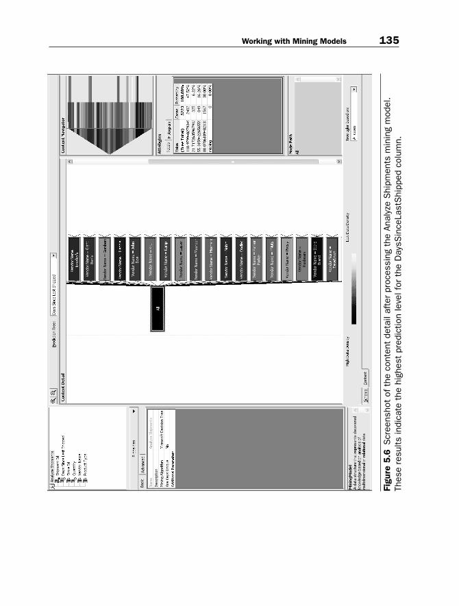
Working with Mining Models 135
Figu
re 5
.6S
cree
nsho
t of
the
con
tent
det
ail a
fter
pro
cess
ing
the
Anal
yze
Shi
pmen
ts m
inin
g m
odel
.Th
ese
resu
lts in
dica
te t
he h
ighe
st p
redi
ctio
n le
vel f
or t
he D
aysS
ince
Last
Shi
pped
col
umn.
ch05.qxd 3/7/05 10:38 AM Page 135
The Content Navigator box—seen in the top-right corner—offersan easy way to see all the mining-model results and drill down into a cer-tain path. The Attributes box shows the totals associated with each node,grouped according to a clustering algorithm. In Figure 5.6, the cursor isselecting the outermost node labeled All. In this example, the attributesare shown for all the cases analyzed.
NOTE: If you did not attach the database file and instead loaded the datausing the LoadSampleData program, you will encounter slightly different sta-tistical results. The results presented in this section are specific to the data-base file available on the book’s Web site.
If you attached your database using the file provided, your processingresults should be the same as the ones we are about to interpret. The firstthing to notice is that the darkest-shaded node is the one where the Ven-dor Name is Store Brand. Nodes that resulted in a higher data density, ormore cases analyzed, will be shaded in a darker color. This result is notsurprising, because 127 of the 500 products available, or 25 percent, arerepresented by the Store Brand. This can be confirmed in Query Ana-lyzer with the following query:
SELECT v.VendorName,(COUNT(ProductID)/500.0) AS 'Percent'
FROM Products p
LEFT JOIN Vendors v ON p.VendorID = v.VendorID
GROUP BY v.VendorName
ORDER BY 'Percent' DESC
If the Store Brand node is double-clicked, the detail pane will showthe next branching of the tree (see Figure 5.7). For the Store Brand Node,the first branching distinguishes between the different stores. If we clickon the node Store ID = 2 and look at the attributes, the value with thehighest probability is 119.33. This indicates that for all products where theVendor name is Store Brand and the Store ID is 2, it is highly probablethat there should be 119 days between shipments.
If we examine the attributes for the remaining nodes, we will see thatpredictions can be made for all the stores. For Store 1, there is one addi-tional branching that distinguishes between a product type of Snack Foodsversus all other product types. When the Store ID is 1, vendor name is StoreBrand, and product type is snack foods, there is a 58 percent probability thatthere will be 60 days between shipments. When we examine the attributes
136 Chapter 5 Data Mining Predictions
ch05.qxd 3/7/05 10:38 AM Page 136

Working with Mining Models 137
Figu
re 5
.7S
cree
nsho
t of
the
Con
tent
Det
ail E
dito
r as
it d
ispl
ays
the
pred
ictio
ns for
day
s si
nce
last
ship
ped.
In t
his
exam
ple,
the
nod
e pa
th is
whe
re S
tore
ID is
2 a
nd t
he v
endo
r na
me
is S
tore
Bra
nd.
ch05.qxd 3/7/05 10:38 AM Page 137
where product type is not snack foods, there is a 43 percent probability thatthere will be 119 days between shipments and a 53 percent probability thatthere will be 85 days between shipments. In this case, we could say that the53 percent probability wins the toss, but that might not always be the bestdecision. This will be discussed further in the next chapter.
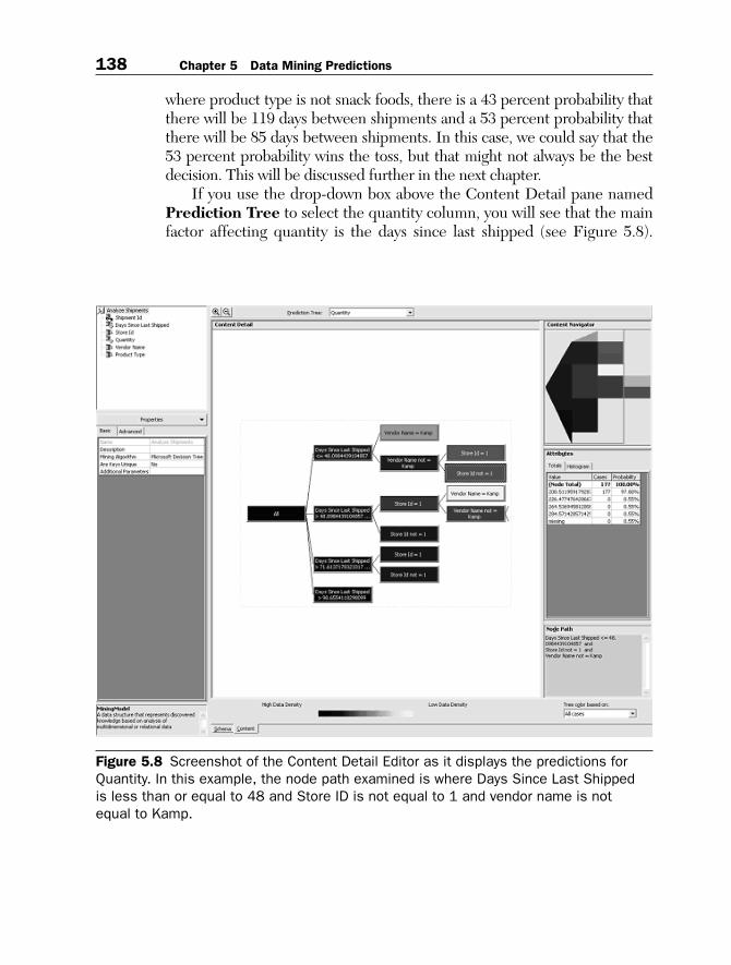
If you use the drop-down box above the Content Detail pane namedPrediction Tree to select the quantity column, you will see that the mainfactor affecting quantity is the days since last shipped (see Figure 5.8).
138 Chapter 5 Data Mining Predictions
Figure 5.8 Screenshot of the Content Detail Editor as it displays the predictions forQuantity. In this example, the node path examined is where Days Since Last Shipped is less than or equal to 48 and Store ID is not equal to 1 and vendor name is not equal to Kamp.
ch05.qxd 3/7/05 10:38 AM Page 138

This is possible because the column DaysSinceLastShipped was definedas an input and a predictable column.
The next factor affecting quantity is the vendor name. In the casewhere the vendor name is NOT Kamp, Store ID is an additional factor. InFigure 5.8 we can see that when the days since last shipped is less than orequal to 48 and the Store ID is NOT 1 and the vendor name is NOTKamp, there is a 98 percent probability that the quantity should be 200.When the Store ID is equal to 1, the prediction drops to a 72 percentprobability that the quantity will be 200.
The next chapter will involve interpreting the results from the miningmodel and then applying the predictions to a new shipment strategy. Thegoal of the new shipment strategy will be to reduce Savings Mart’s opera-tional costs by reducing the total number of shipments.
Summary
■ The technology known as data warehousing has developed as a meansof making use of the huge quantities of data available these days. In ad-dition to storing all this data, data mining is needed to make useful pre-dictions about it. Analysis Services, a separate install for SQL Server2000, offers data-mining capabilities in an easy-to-use and scalable way.
■ This chapter is one of two that examines the effort of a fictional dis-count retailer named Savings Mart to improve its operational efficien-cies. A sample application named LoadSampleData, provided on thebook’s Web site, allows readers to generate a unique dataset for thedata-mining model. Optionally, the reader can also attach a database fileprovided on the Web site.
■ One of the biggest problems affecting successful data mining is invalidor incorrect data. Therefore, the process of cleaning a database is oftenthe most time-consuming aspect of preparing a dataset.
■ We step through the process of creating a mining model using AnalysisServices. This involves creating a database, naming the data source, andusing the mining-model wizard to create the actual model.
■ Once a model is created, it can be trained with a training dataset to pro-duce prediction results. The training dataset in this chapter representsone year’s worth of purchases and shipments to all five stores. These re-sults will be the basis for a Windows service created in the next chapter.
Summary 139
ch05.qxd 3/7/05 10:38 AM Page 139

ch05.qxd 3/7/05 10:38 AM Page 140