Chapter 5 Capital Income Taxation - Keio Income Taxation.pdf · Chapter 5 Capital Income Taxation ....
29
Lectures on Public Finance Part 2_Chap 5, 2016 version P.1 of 29 Last updated 19/4/2016 Chapter 5 Capital Income Taxation 5.1 Taxation of Income from Capital 1 The Ramsey rule for efficient taxation provides a justification for taxing income from capital differently from income from labor, since governments are advised to set tax rates inversely proportional to supply elasticities. That is, with L t the rate of taxation of labor income and K t the rate of taxation of income from capital, the Ramsey rule proposes that tax rates be set so that , SL SK K L t t ε ε = (1) where ) , ( K L i Si = ε is the supply elasticity 2 . The supply elasticities in expression (1) reflect opportunities to leave a tax jurisdiction. If capital can readily leave, the elasticity of supply of capital SK ε is high. Conversely, if labor cannot leave, the elasticity of supply of labor SL ε is low. The Ramsey rule therefore implies that the rate of taxation on income from capital should be lower than the rate of taxation on income from labor 3 . If capital in a tax jurisdiction is part of a broader capital market and can simply leave in response to a tax on income from capital, the tax rate on capital indicated by the Ramsey rule is zero 4 . The home bias in investment Possibilities for taxing capital depend on the willingness of investors to hold assets outside their tax jurisdiction. Investors often seem reluctant to hold foreign assets, which results in a “home bias” in asset holdings. The home bias may be due to investors’ believing that they are better informed about investments in their home markets. Investors may also trust their own 1 This part draws from Hillman (2003) Chap 7, pp.493-6. 2 This statement of the Ramsey rule is based on infinite elasticities on the other side of the market (here demand elasticities) and independence between markets so that a tax in one market does not affect tax revenue in other markets. 3 Personal income taxes usually have more than one rate. In expression (1) for the Ramsey rule, there is one rate of taxation for income depending on the source of income. That is, we are note now asking questions about the structure of taxation for different levels of income. Nor are we asking questions about different rates of taxation for different people implied by the Ramsey rule. 4 If the broader market, for example, offers a return of 5 percent, any attempt to tax capital to reduce the local return below 5 percent will lead investors to move their capital outside the jurisdiction where they can obtain the 5 percent return.
Transcript of Chapter 5 Capital Income Taxation - Keio Income Taxation.pdf · Chapter 5 Capital Income Taxation ....
Lectures on Public Finance Part 2_Chap 5, 2016 version P.1 of 29 Last updated 19/4/2016
Chapter 5 Capital Income Taxation
5.1 Taxation of Income from Capital1
The Ramsey rule for efficient taxation provides a justification for taxing income from capital differently from income from labor, since governments are advised to set tax rates inversely proportional to supply elasticities. That is, with Lt the rate of taxation of labor income and
Kt the rate of taxation of income from capital, the Ramsey rule proposes that tax rates be set so
that
,SL
SK
K
L
tt
εε
= (1)
where ),( KLiSi =ε is the supply elasticity2. The supply elasticities in expression (1) reflect
opportunities to leave a tax jurisdiction. If capital can readily leave, the elasticity of supply of capital SKε is high. Conversely, if labor cannot leave, the elasticity of supply of labor SLε
is low. The Ramsey rule therefore implies that the rate of taxation on income from capital should be lower than the rate of taxation on income from labor3. If capital in a tax jurisdiction is part of a broader capital market and can simply leave in response to a tax on income from capital, the tax rate on capital indicated by the Ramsey rule is zero4. The home bias in investment Possibilities for taxing capital depend on the willingness of investors to hold assets outside their tax jurisdiction. Investors often seem reluctant to hold foreign assets, which results in a “home bias” in asset holdings. The home bias may be due to investors’ believing that they are better informed about investments in their home markets. Investors may also trust their own
1 This part draws from Hillman (2003) Chap 7, pp.493-6. 2 This statement of the Ramsey rule is based on infinite elasticities on the other side of the market (here demand elasticities) and independence between markets so that a tax in one market does not affect tax revenue in other markets. 3 Personal income taxes usually have more than one rate. In expression (1) for the Ramsey rule, there is one rate of taxation for income depending on the source of income. That is, we are note now asking questions about the structure of taxation for different levels of income. Nor are we asking questions about different rates of taxation for different people implied by the Ramsey rule. 4 If the broader market, for example, offers a return of 5 percent, any attempt to tax capital to reduce the local return below 5 percent will lead investors to move their capital outside the jurisdiction where they can obtain the 5 percent return.
Lectures on Public Finance Part 2_Chap 5, 2016 version P.2 of 29 Last updated 19/4/2016
government more than foreign governments to protect their ownership rights. The home bias reduces the supply elasticity of capital and, through the Ramsey rule, increases the efficient tax on income from capital relative to income from labor. Social justice A government may believe that social justice requires taxing income from capital at a higher rate than income from labor. The presence of capital markets that extend beyond the government’s tax jurisdiction, however, limits the scope for taxing income from capital. If capital can leave the jurisdiction to escape the tax, a government has no choice but to set low taxes on income from capital and high taxes on income from labor because, by attempting to tax income from capital, the government ends up with little or no capital to tax. Portfolio investment and real assets When people choose to save rather than consume, resources can be invested to create capital. The capital can be human capital invested in the skills, ability, and knowledge of a person or can take the form of physical capital. When we refer to movement of capital out of a tax jurisdiction, we may mean physical capital, and also human capital. Machinery and equipment move as firms relocate their operations to other tax jurisdictions, and high human-capital people might also move to escape taxes. People are also described as investing when they buy stocks or shares in a company, or when they buy government or corporate bonds. Such portfolio investment changes the ownership of assets but does not create new assets. Where people hold their personal investment portfolios affects their tax obligations, through the different taxes that different government levy in their jurisdictions. Where people “hold” their asset portfolios is a legal fiction. For example, a portfolio of shares in U.S., European, and Japanese companies can be “held” in a Caribbean island where low taxes (or no taxes) are levied on income from portfolio investments of nonresidents. The government of the Caribbean island gains tax revenue by attracting offices of “off-share” portfolio management companies and through legal fees. Locations with low or no taxes on nonresidents’ income from portfolio investment are known as tax havens5. The presence of tax havens limits other governments’ abilities to tax income from ownership of capital. When taxes on income from capital increase, no actual capital may leave the tax jurisdiction, but an asset “portfolio” may leave, by the transfer of the location of ownership of the asset portfolio to a tax haven. We therefore need to distinguish between investment as financial capital and investment as 5 The financial press lists information about the values of shares in investment companies in tax havens.
Lectures on Public Finance Part 2_Chap 5, 2016 version P.3 of 29 Last updated 19/4/2016
physical capital. In both cases, capital can be mobile. However, portfolio investment is more mobile than physical investment. Residence-based taxation To avoid loss of tax revenue by transfer of assets to foreign locations, governments may define tax liability based on the location of residence of the taxpayer and not on the location of the office of the investment company that holds assets in the name of the taxpayer. However, even with residence-based taxation, assets can be held abroad beyond the reach of the taxation authorities, if foreign banks maintain a policy of confidentiality regarding identities of account holders. Taxpayers are then engaging in tax evasion by holding asset portfolios in foreign tax havens. Dynamic inconsistency Taxation of income from capital is subject to the problem of dynamic inconsistency. To explain this problem, we observe that, even though financial capital is in general very mobile, the physical capital in place after an investment has been made is less mobile. Often, after an investment in physical capital has been made (a factory has been built), the capital cannot readily move elsewhere. The supply elasticity of capital after the investment has been made is then zero. The supply elasticity of capital before the investment is made, may however be, quite high because of alternative locations where the investment can be made and also because of the option not to make the investment at all. Therefore, the supply elasticity of capital before the investment decision has been made is in general greater than after the investment has been made. A government that wishes to apply the Ramsey rule for efficient taxation could announce a low rate of taxation of income from capital before an investment is made, to reflect the high supply elasticity of capital. However, after the investment has been made, the Ramsey rule calls for a high rate of taxation on income from the investment because of the subsequent low (or zero) supply elasticity of capital. Announcement by a government of a low rate of taxation on income from capital is therefore dynamically inconsistent. The low tax announced today will not be the tax rate that the government will wish to apply tomorrow. The announcement of a low tax rate before the investment has been made will therefore not be credible to investors because investors know that it is in the interest of the government to increase the tax rate after an investment has been made. If the announcement of a low tax rate is not credible, investments will not be made, because of the anticipation by investors of high taxes in the future. There is a saying that the best tax is an old tax. That is, it is wise for government not to change taxes. Stable taxes allow investment decisions to be made without the uncertainty of
Lectures on Public Finance Part 2_Chap 5, 2016 version P.4 of 29 Last updated 19/4/2016
having to predict future government tax policy. Investment is by nature subject to uncertainty. Uncertainty about taxes increases the uncertainty that firms face when deciding whether to invest. A reputation for stable taxes is a way of establishing and confirming a commitment not to take advantage of capital that becomes immobile after an investment has been made. Therefore, there are benefits from maintaining an unchanged rate of taxation on income from capital. When tax rates on income from capital are increased, the credibility that tax rates will not be changed again in the future is lost, and investors can become reluctant to invest. Similar considerations affect taxation of natural resources. After an exploration company has discovered an oil deposit, the income earned from the oil is a rent because there is no way to use the asset other than to extract oil. The Ramsey rule calls for appropriative taxes on rents because rents are returns from investments for which supply elasticities are zero. We see the time-inconsistency problem about taxation intentions that confronts an oil exploration company. The elasticity of supply of capital for oil exploration is high, which by the Ramsey rule calls for low tax rates on future income from successful exploration. However, after oil is found, the Ramsey rule calls for high taxes. Because of the time-inconsistency problem, the rule that an old (stable) tax is a good tax also applies to incentives for oil exploration, and exploration for other natural resources. The Effects of Taxation on Savings6
In most countries, income taxation bears both on labor income and on income from savings. With perfect financial markets, taxation of labor income only changes the savings rate in that the latter depends on permanent income. We will focus here on the effect of taxation of income from savings on the time profile of consumption over the life cycle. We will therefore start by neglecting the taxation of labor income. We also assume an exogenous interest rate, which neglects general equilibrium effects. Theoretical Analysis
Consider a consumer who lives two periods and whose labor supply is inelastic. He gets in the first period a wage w, consumes some part of it, and saves the rest according to
wEC =+1
In the second period, he does not work7 and consumes the net income from his savings. Given an interest rate r and taxation of income from savings at a proportional rate t, his budget
6 This part draws from Salanié (2003) Chap 2, pp.45-9. 7 Thus the first period could be the active period of life and the second retirement.
Lectures on Public Finance Part 2_Chap 5, 2016 version P.5 of 29 Last updated 19/4/2016
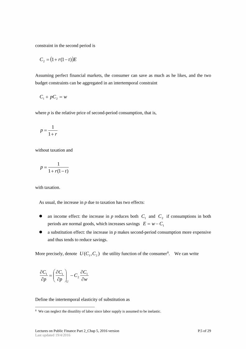
constraint in the second period is
( )EtrC )1(12 −+=
Assuming perfect financial markets, the consumer can save as much as he likes, and the two budget constraints can be aggregated in an intertemporal constraint
wpCC =+ 21
where p is the relative price of second-period consumption, that is,
rp
+=
11
without taxation and
)1(11
trp
−+=
with taxation.
As usual, the increase in p due to taxation has two effects: an income effect: the increase in p reduces both 1C and 2C if consumptions in both
periods are normal goods, which increases savings 1CwE −=
a substitution effect: the increase in p makes second-period consumption more expensive and thus tends to reduce savings.
More precisely, denote ),( 21 CCU the utility function of the consumer8. We can write
wCC
pC
pC
U ∂∂
−
∂∂
=∂∂ 1
211
Define the intertemporal elasticity of substitution as 8 We can neglect the disutility of labor since labor supply is assumed to be inelastic.

Lectures on Public Finance Part 2_Chap 5, 2016 version P.6 of 29 Last updated 19/4/2016
UpCC
∂
∂=
log)log( 21σ
First note that since Hicksian demands are the derivatives of the expenditure function ),( Upe
with respect to prices, the equality
),(),(),( 21 UpeUppCUpC =+
implies by differentiating in p that
021 =
∂∂
+
∂∂
UU pCp
pC
Since by definition
UU pC
pC
∂∂
−
∂∂
=loglog
loglog 21σ
we obtain
UU pC
pCw
pC
CCp
∂∂
=
∂∂
+=
loglog
loglog1 1
2
1
21
σ
and
σep
C
U
=
∂∂
loglog 1
where wpCwEe 2== denotes the savings rate.
We also have
Lectures on Public Finance Part 2_Chap 5, 2016 version P.7 of 29 Last updated 19/4/2016
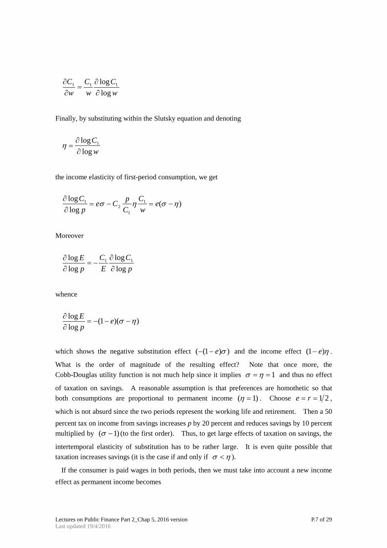
wC
wC
wC
loglog 111
∂∂
=∂∂
Finally, by substituting within the Slutsky equation and denoting
wC
loglog 1
∂∂
=η
the income elasticity of first-period consumption, we get
)(loglog 1
12
1 ησησ −=−=∂∂ e
wC
CpCe
pC
Moreover
pC
EC
pE
loglog
loglog 11
∂∂
−=∂∂
whence
))(1(loglog ησ −−−=
∂∂ e
pE
which shows the negative substitution effect ))1(( σe−− and the income effect η)1( e− .
What is the order of magnitude of the resulting effect? Note that once more, the Cobb-Douglas utility function is not much help since it implies 1==ησ and thus no effect
of taxation on savings. A reasonable assumption is that preferences are homothetic so that both consumptions are proportional to permanent income )1( =η . Choose 21== re ,
which is not absurd since the two periods represent the working life and retirement. Then a 50 percent tax on income from savings increases p by 20 percent and reduces savings by 10 percent multiplied by )1( −σ (to the first order). Thus, to get large effects of taxation on savings, the
intertemporal elasticity of substitution has to be rather large. It is even quite possible that taxation increases savings (it is the case if and only if ησ < ).
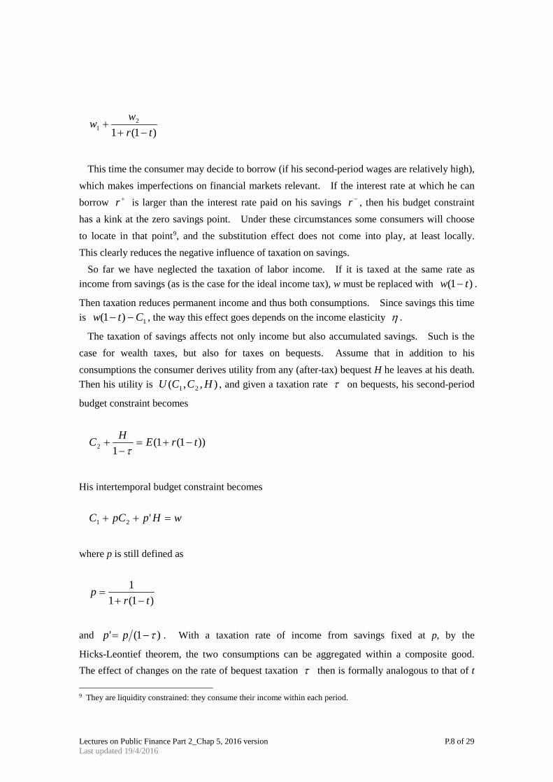
If the consumer is paid wages in both periods, then we must take into account a new income effect as permanent income becomes
Lectures on Public Finance Part 2_Chap 5, 2016 version P.8 of 29 Last updated 19/4/2016
)1(12
1 trww
−++
This time the consumer may decide to borrow (if his second-period wages are relatively high),
which makes imperfections on financial markets relevant. If the interest rate at which he can borrow +r is larger than the interest rate paid on his savings −r , then his budget constraint has a kink at the zero savings point. Under these circumstances some consumers will choose to locate in that point9, and the substitution effect does not come into play, at least locally. This clearly reduces the negative influence of taxation on savings.
So far we have neglected the taxation of labor income. If it is taxed at the same rate as income from savings (as is the case for the ideal income tax), w must be replaced with )1( tw − .
Then taxation reduces permanent income and thus both consumptions. Since savings this time is 1)1( Ctw −− , the way this effect goes depends on the income elasticity η .
The taxation of savings affects not only income but also accumulated savings. Such is the case for wealth taxes, but also for taxes on bequests. Assume that in addition to his consumptions the consumer derives utility from any (after-tax) bequest H he leaves at his death. Then his utility is ),,( 21 HCCU , and given a taxation rate τ on bequests, his second-period
budget constraint becomes
))1(1(12 trEHC −+=−
+τ
His intertemporal budget constraint becomes
wHppCC =++ '21
where p is still defined as
)1(11
trp
−+=
and )1(' τ−= pp . With a taxation rate of income from savings fixed at p, by the
Hicks-Leontief theorem, the two consumptions can be aggregated within a composite good. The effect of changes on the rate of bequest taxation τ then is formally analogous to that of t 9 They are liquidity constrained: they consume their income within each period.
Lectures on Public Finance Part 2_Chap 5, 2016 version P.9 of 29 Last updated 19/4/2016
on savings. This analysis of bequests is only half convincing, however. Whether bequests are planned or accidental (due to early deaths) is a controversial issue. In any case the taxation of bequests, like wealth taxes, collects very small amounts of tax revenues in most countries.
Empirical Results
In the 1970s econometricians tried to estimate the elasticity of aggregate consumer savings to the after-tax interest rate. Apart from Boskin (1978) who obtained a value close to 0.4, most estimates were close to zero. This quasi-consensus was shaken by a paper of Summers (1981). Using the calibration of a life-cycle model in a growing economy, Summers showed that any choice of parameters compatible with the observed ratio of wealth to income implied a large elasticity of savings to the interest rate. More recent work, however, has showed that Summers’s result is fragile.
The literature turned in the 1980s to the estimation of Euler equations derived from the intertemporal optimization of consumers; this yielded values for the intertemporal elasticity of substitution σ . Studies done on macroeconomic data have yielded small values for σ . More credible estimations on individual data suggest that σ is nonnegligible but lower than
one (which is its value for a Cobb-Douglas utility function), which implies a very small elasticity of savings to the interest rate.
Finally, many authors have used the existence of investments that are favored by taxation. Most of these studies use data from the United States, where it is possible to use Individual Retirement Accounts (IRA) and 401(k) funds to save into pension funds and deduct the amount saved from taxable income. These funds have been very successful, but the important question is whether the money that went into them would have been saved anyway or not. The studies are not unanimously conclusive, but it seems that total savings was only moderately stimulated by the favorable tax treatment of these funds.
A general lesson of this literature10 is that taxation is unlikely to have a large impact on total savings, although it clearly plays an important role in determining where the money is invested.
Taxation and Risk-Taking11
Taxation is often said to discourage risk-taking, since it confiscates part of the return to risky
activities such as setting up a business or investing in shares. Domar and Musgrave (1944) however noted that taxation transforms government into a sleeping partner who absorbs part of the risk, which may in fact encourage risk-taking. We will revisit this argument following
10 Bernheim (2002) contains a much more detailed discussion. 11 This part draws from Salanié (2003) Chap 2, pp.49-52.
Lectures on Public Finance Part 2_Chap 5, 2016 version P.10 of 29 Last updated 19/4/2016
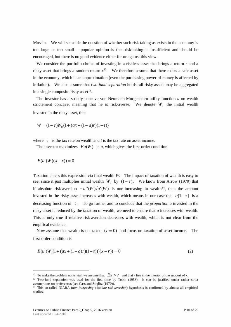
Mossin. We will set aside the question of whether such risk-taking as exists in the economy is too large or too small – popular opinion is that risk-taking is insufficient and should be encouraged, but there is no good evidence either for or against this view.
We consider the portfolio choice of investing in a riskless asset that brings a return r and a risky asset that brings a random return x12. We therefore assume that there exists a safe asset in the economy, which is an approximation (even the purchasing power of money is affected by inflation). We also assume that two-fund separation holds: all risky assets may be aggregated in a single composite risky asset13.
The investor has a strictly concave von Neumann-Morgenstern utility function u on wealth strictement concave, meaning that he is risk-averse. We denote 0W the initial wealth
invested in the risky asset, then
))1)()1((1()1( 0 traaxWW −−++−= τ
where τ is the tax rate on wealth and t is the tax rate on asset income.
The investor maximizes )(WEu in a, which gives the first-order condition
0)))(('( =− rxWuE
Taxation enters this expression via final wealth W. The impact of taxation of wealth is easy to see, since it just multiplies initial wealth 0W by )1( τ− . We know from Arrow (1970) that
if absolute risk-aversion )(')('' WuWu− is non-increasing in wealth14, then the amount invested in the risky asset increases with wealth, which means in our case that )1( τ−a is a
decreasing function of τ . To go further and to conclude that the proportion a invested in the
risky asset is reduced by the taxation of wealth, we need to ensure that a increases with wealth. This is only true if relative risk-aversion decreases with wealth, which is not clear from the empirical evidence.
Now assume that wealth is not taxed )0( =τ and focus on taxation of asset income. The
first-order condition is
0)))))(1)()1((1(('( 0 =−−−++ rxtraaxWuE (2)
12 To make the problem nontrivial, we assume that rEx > and that r lies in the interior of the support of x. 13 Two-fund separation was used for the first time by Tobin (1958). It can be justified under rather strict assumptions on preferences (see Cass and Stiglitz (1970)). 14 This so-called NIARA (non-increasing absolute risk-aversion) hypothesis is confirmed by almost all empirical studies.
Lectures on Public Finance Part 2_Chap 5, 2016 version P.11 of 29 Last updated 19/4/2016
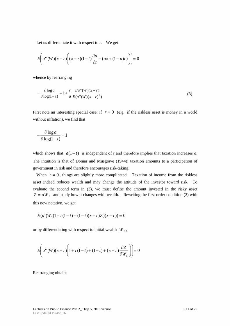
Let us differentiate it with respect to t. We get
0))1(()1)(())(('' =
−+−
∂∂
−−− raaxtatrxrxWuE
whence by rearranging
)))((''())((''1
)1log(log
2rxWuErxWEu
ar
ta
−
−+=
−∂∂
− (3)
First note an interesting special case: if 0=r (e.g., if the riskless asset is money in a world
without inflation), we find that
1)1log(
log=
−∂∂
−t
a
which shows that )1( ta − is independent of t and therefore implies that taxation increases a.
The intuition is that of Domar and Musgrave (1944): taxation amounts to a participation of government in risk and therefore encourages risk-taking.
When 0≠r , things are slightly more complicated. Taxation of income from the riskless
asset indeed reduces wealth and may change the attitude of the investor toward risk. To evaluate the second term in (3), we must define the amount invested in the risky asset
0aWZ = and study how it changes with wealth. Rewriting the first-order condition (2) with
this new notation, we get
0)))())(1()1(1(('( 0 =−−−+−+ rxZrxttrWuE
or by differentiating with respect to initial wealth 0W ,
0)()1()1(1))((''0
=
∂∂
−+−+−+−WZrxttrrxWuE
Rearranging obtains
Lectures on Public Finance Part 2_Chap 5, 2016 version P.12 of 29 Last updated 19/4/2016
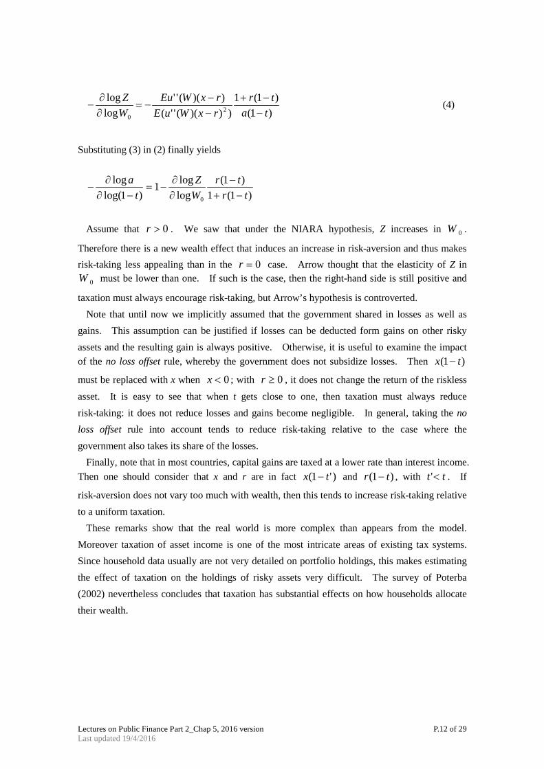
)1()1(1
)))((''())((''
loglog
20 ta
trrxWuErxWEu
WZ
−−+
−−
−=∂∂
− (4)
Substituting (3) in (2) finally yields
)1(1)1(
loglog1
)1log(log
0 trtr
WZ
ta
−+−
∂∂
−=−∂
∂−
Assume that 0>r . We saw that under the NIARA hypothesis, Z increases in 0W .
Therefore there is a new wealth effect that induces an increase in risk-aversion and thus makes risk-taking less appealing than in the 0=r case. Arrow thought that the elasticity of Z in
0W must be lower than one. If such is the case, then the right-hand side is still positive and
taxation must always encourage risk-taking, but Arrow’s hypothesis is controverted. Note that until now we implicitly assumed that the government shared in losses as well as
gains. This assumption can be justified if losses can be deducted form gains on other risky assets and the resulting gain is always positive. Otherwise, it is useful to examine the impact of the no loss offset rule, whereby the government does not subsidize losses. Then )1( tx −
must be replaced with x when 0<x ; with 0≥r , it does not change the return of the riskless
asset. It is easy to see that when t gets close to one, then taxation must always reduce risk-taking: it does not reduce losses and gains become negligible. In general, taking the no loss offset rule into account tends to reduce risk-taking relative to the case where the government also takes its share of the losses.
Finally, note that in most countries, capital gains are taxed at a lower rate than interest income. Then one should consider that x and r are in fact )'1( tx − and )1( tr − , with tt <' . If
risk-aversion does not vary too much with wealth, then this tends to increase risk-taking relative to a uniform taxation.
These remarks show that the real world is more complex than appears from the model. Moreover taxation of asset income is one of the most intricate areas of existing tax systems. Since household data usually are not very detailed on portfolio holdings, this makes estimating the effect of taxation on the holdings of risky assets very difficult. The survey of Poterba (2002) nevertheless concludes that taxation has substantial effects on how households allocate their wealth.
Lectures on Public Finance Part 2_Chap 5, 2016 version P.13 of 29 Last updated 19/4/2016
The Taxation of Capital15
Labor income only comprises about two-thirds of GDP, while one-third goes to capital. Taxation
of capital therefore deserves its own analysis. It is a very vast subject, since many things go under
the name of capital. The common element to all of these is that capital is accumulated savings,
whether it be physical capital (machines and buildings used for production, but also housing held by
families) or financial capital (bank and financial assets, e.g., bonds and shares). Thus taxation of
capital in fact involves two sorts of taxes:
taxes on the stock of capital like the wealth tax, the tax on bequests, property taxes
taxes on the income form savings, such as the corporate income tax16, taxation of interest and
dividends, and the taxation of capital gains17.
The economic analysis of these two cases in fact is very similar, since capital stocks stem from
accumulated savings. Thus the distinction will play no role in this section.
The standpoint adopted here is that of optimal taxation. Thus our main concern here is with the
optimal level of capital taxation. However, we will also return to the incidence of capital taxation.
Here we neglect considerations linked to risk. This makes the analysis much less realistic but also
much more tractable.
In many European countries the press and some politicians complain that the taxation rate of
capital goes down while taxation of labor income seems to increase inexorably. This is deemed
unfair, since a common (but simplistic) theory of incidence suggests that workers pay the tax on
labor income and capitalists pay the tax on capital. This is also thought to encourage substitution of
capital for labor, thus reducing labor demand. Therefore the relative decline of the taxation of
capital would be partly responsible for high unemployment and low wages.
As often in the theory of taxation, theoretical results are quite remote from popular discourse.
We will see in this section that at least to a first approximation, there is no strong reason to tax
capital at all: the optimal tax rate on capital is zero! This a priori surprising result actually is an old
theme in economic literature. It is linked to the optimality of a consumption tax. As is easily seen
by writing the intertemporal budget constraint of a worker-consumer who receives and leaves no
bequest,
∑∑== +
=+
T
tt
tT
tt
t
rLw
rC
11 )1()1( (5)
15 This part draws heavily from Salanié (2003) Chap6, pp.121-40. 16 Although the question of what the corporate income tax actually taxes is controversial. 17 The stock-flow distinction is not very clear when it comes to capital gains; however, they are usually taxes as income.
Lectures on Public Finance Part 2_Chap 5, 2016 version P.14 of 29 Last updated 19/4/2016
a tax on consumption is equivalent to a tax that bears on labor income only, to the exclusion of
income from savings.
Applying Classical Results
The effect of taxation of income from savings is to increase the price of future consumption
relative to that of current consumption. Thus what matters is whether we should tax future
consumption more than current consumption. The results seem to apply directly to this problem,
since we may consider consumptions at various dates as many as different goods.
Ramsey’s formula gives us a first guide. With a representative consumer, the Corlett-Hague
result shows that a higher tax on future consumptions may be in order if they are more
complementary to leisure than current consumption. This in principle is an empirically testable
proposition: Does a permanent wage increase translate (for fixed utility) into an increase of future
consumptions smaller than that in current consumption? Unfortunately, we have no convincing
answer to this question. If future consumptions and current consumption are equally
complementary to leisure but individuals are heterogeneous, then Ramsey’s formula indicates that
future consumption should be discouraged more if the rich tend to defer their consumption more
than the poor. Observation shows convincingly that the rich have a higher propensity to save than
the poor, which seems to provide us with a second argument for taxing capital.
However, Ramsey’s model in fact is very restrictive, as it only allows for proportional labor
income taxation. Now turn to the Atkinson-Stiglitz result on the role of indirect taxation with an
optimal nonlinear income tax. This theorem tells us that if the utility function of consumers is
weakly separable, so that it can be written
),,,),,,((~),,,,,,( 1111 wLLCChUwLLCCU TTTT =
then all consumptions should be taxed at the same rate and income from savings should not be taxed
at the optimum. Under this separability hypothesis, the targeting principle applies: it may well be
that the rich save more, but this is because they have higher incomes, and that comes from their
higher productivity. Thus the optimal trade-off between equity and efficiency can be attained by
taxing only labor income.
The fact that the Atkinson and Stiglitz result neglects inherited wealth seems the most relevant
here: if consumer-workers come to life with different productivities and different bequests, then the
latter should be taxed at the optimum. There is indeed no relevant difference between endowments
at birth, whether they consist in higher productivity or a higher bequest. However, this argument
Lectures on Public Finance Part 2_Chap 5, 2016 version P.15 of 29 Last updated 19/4/2016
neglects the effect of capital taxation on the decisions of the person who leaves the bequest.
Taxation of bequests becomes more problematic if they are planned by altruistic donors.
Capital Accumulation
For simplicity, we assume that every generation has only one type of agent: redistributive
considerations are not essential here since we focus on the capital accumulation process. As before,
generations grow at rate n; labor supply is now assumed to be inelastic (each young person supplies
one unit of labor). Capital does not depreciate, and there is no technical progress. We start the
analysis by assuming that there is no taxation to begin with. Recall that we are in a closed economy,
so savings must directly feed investment.
With an inelastic labor supply, the representative agent of generation t maximizes ),( 1,0 +tyt CCU
under his budget constraint
+=
=+
++ ttt
ttyt
SrCwSC
)1( 11,0
where tS is the savings of generation t. We obtain the intertemporal budget constraint as
tt
tyt w
rC
C =+
++
+
1
1,0
1
The first-order condition is
10
1)(')('
++= tt
ty rCUCU
which generates demand functions ),( 1+tt rwC and savings
),(),( 11 ++ −= ttyttt rwCwrwS
We still denote ),( LKF production (net of capital), and we denote )1,()( kFkf = net
production per capita. As usual, profit maximization gives factor incomes:
Lectures on Public Finance Part 2_Chap 5, 2016 version P.16 of 29 Last updated 19/4/2016
=−=
)(')(')(
tt
ttttkfr
kfkkfw
where we used the notation ttt LKk = .
Finally, equilibrium on the market for capital implies the equality between the savings of the young tS and the capital stock in the next period18. Taking into account demographic growth,
this gives
))('),(')((),()1( 111 +++ −==+ ttttttt kfkfkkfSrwSnk
This equation defines the dynamics of the capital accumulation process. Unfortunately, it is very nonlinear, which raises several difficulties. First note that 1+tk appears on both sides of the
equation, so the dynamics is only defined implicitly. We will assume here that we can in fact extract a dynamic mapping )(1 tt kgk =+ . Even then, this system may not be stable. Now
assume that there exists a unique solution *k of
))('),(')(()1( ***** kfkfkkfSnk −=+
This solution is locally stable if
1)(' * <kg
that is, if
1')(''1
')(''*
**
<−+
−
r
w
SkfnSkfk
Then the per capita capital stock converges (at least locally) to *k , which defines the steady state equilibrium where capital intensity is constant and the stock of capital grows at the same rate n as the
population.
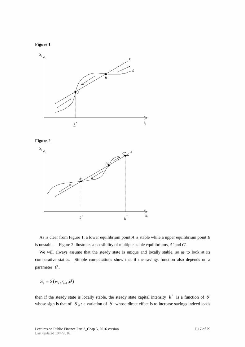
The graphs may illustrate this solution concept visually.
18 The capital stock of period t is recycled, and some of it may be consumed –remember that there is only one good in the economy.
Lectures on Public Finance Part 2_Chap 5, 2016 version P.17 of 29 Last updated 19/4/2016
Figure 1
tS
*k
S
B
A
k
kt
Figure 2
tS
*k
B’
A’
k
C’
*k
kt
As is clear from Figure 1, a lower equilibrium point A is stable while a upper equilibrium point B
is unstable. Figure 2 illustrates a possibility of multiple stable equilibriums, A’ and C’.
We will always assume that the steady state is unique and locally stable, so as to look at its
comparative statics. Simple computations show that if the savings function also depends on a
parameter θ ,
),,( 1 θ+= ttt rwSS
then if the steady state is locally stable, the steady state capital intensity *k is a function of θ whose sign is that of θ'S : a variation of θ whose direct effect is to increase savings indeed leads
Lectures on Public Finance Part 2_Chap 5, 2016 version P.18 of 29 Last updated 19/4/2016
to an increase in capital intensity.
The uniqueness and local stability assumptions imposed on the dynamic system are very strong: in general, one cannot exclude indeterminacies (several solutions in 1+tk for a given tk ) and/or
cyclical or even chaotic dynamics.
Is the steady state optimal? Optimality is rather easy to define if we focus on stationary
trajectories, where all per capita allocations are constant. Then all generations have the same utility,
and we naturally seek to maximize the utility of any of them. Thus consider a stationary allocation
with capital intensity k. Our old friend the benevolent and omniscient planner only faces one
constraint: since he needs nk, given population growth, to keep the capital intensity unchanged, he only has ))(( nkkf − to share between the old and the young in any given period. Since the old
at each time are )1( n+ times fewer than the young, we must therefore have
nkkfn
CCY −=
++ )(
10
If we maximize ),( 0CCU y under this constraint, obviously we first need to maximize
))(( nkkf − , which gives
nkfr == )('
At the social optimum, capital intensity must be such that the interest rate equals the rate of growth
of the population. This is called the golden rule, and it defines a capital intensity Gk .
Can we compare the optimum Gk and the steady state *k ? Unfortunately, there is no reason why these two capital intensities should coincide. Assume, for instance, that the utility has the
Cobb-Douglas form
00 log)1(log),( CaCaCCU yy −+=
and that the production function also is a Cobb-Douglas:
αα −= 1),( LKLKF
Then

Lectures on Public Finance Part 2_Chap 5, 2016 version P.19 of 29 Last updated 19/4/2016
αkkf =)(
The consumption and savings functions are very simple:
−=−+=
=
waSwarC
awC y
)1()1)(1(0
The dynamics of capital intensities is
εα tt kank )1)(1()1(1 −−=++
which indeed converges to a steady state given by
)1(1
*
1)1)(1( αα −
+−−
=n
ak
The golden rule gives
nk G =−1)( αα
or
)1(1 αα −
=
nk G
It is easily seen that Gk may be smaller or greater19 than *k . Moreover no reasonable condition will make them equal: in general, the steady state is not optimal20.
When *kk G < , one can even improve the utility of all generations. Just assume that just after
19 The reader may check that seems more likely with “reasonable” values of a, and n, but once again, this model is not particularly realistic. 20 This is no violation of the first welfare theorem: here we have an infinity of agents indexed with their date of birth, whereas the proof of the first theorem heavily relies on the assumption that the number of agents is finite.
Lectures on Public Finance Part 2_Chap 5, 2016 version P.20 of 29 Last updated 19/4/2016
production at some date T, the government decides to release )( * Gkk − for consumption and to
then maintain the capital intensity at Gk . The quantity of good available for consumption in period T is
))(1()()()( ***** GGG kknnkkfnkkkkf −++−=−−+
which is larger than ))(( ** nkkf − : both generations present at T can consume more. At later
dates the quantity available for consumption is
** )()( nkkfnkkf GG −>−
by the definition of the golden rule, and here again all generations alive at these dates can consume
more. With such excess accumulation of capital, we say that the economy is dynamically
inefficient: there exists a reallocation that improves the utility of all generations21. Otherwise, we
say that the economy is dynamically efficient – which does not mean that the level of capital is
optimal, since Gkk ≤* . Let us now return to the taxation of capital. Any tax (or subsidy) on capital affects savings and
therefore capital accumulation. If the steady state is not optimal, such a tax can thus bring the
economy closer to the golden rule. If, for instance, we tax capital at rate τ and we redistribute
the tax revenue to the young (with a transfer yT ) and to the old (with a transfer 0T ), then the
consumer’s budget constraints become
+−+=
+=+
00 ))1(1( TSrCTwSC yy
τ
or in the intertemporal form
)1(1)1(1
00
ττ −+++=
−++
rT
TwrC
C yy
so that savings become
21 Abel et al. (1989) study empirically the accumulation process in the main developed countries. They conclude that the economy is dynamically efficient in each of these countries, which suggests that they have too little capital.

Lectures on Public Finance Part 2_Chap 5, 2016 version P.21 of 29 Last updated 19/4/2016
−
−+++−+= )1(,
)1(10 τ
τr
rT
TwCTwS yyy
Transfers must, of course, balance the government’s budget constraint, which is
n
Srn
TTy +
=+
+11
0 τ
since the tax collects Srτ on each old individual and the old are )1( n+ times fewer than the
young in each period.
Creating such a tax changes the capital accumulation process through
Skn =+ )1(
We could pursue with complicated computations, but let us focus on the effects involved instead.
The creation of the tax has, as usual, two opposite effects on savings: the income effect increases
savings, and the substitution effect reduces it22. A transfer to the old tends to reduce savings since
it helps finance second-period consumption. Finally, a transfer to the young increases savings in
the reasonable case where the marginal propensity to consume is below one. There are thus five
effects to account for, and two independent instruments (since τ , yT , and 0T are linked by the
government’s budget constraint).
For simplicity, return to the case where the utility function is Cobb-Douglas; then the income
effect and the substitution effect cancel out and we have
)1(1
))(1( 0
τ−+−+−=
raT
TwaS y
First assume that the revenue from taxing capital is entirely given to the young: 00 =T and
)1( nSrTy += τ . Then we get
)1()1(1
)1(nra
waS+−−
−=
τ
22 There is here a third effect due to the discounting of the transfer to the old; this tends to reduce savings if 0T is positive.
Lectures on Public Finance Part 2_Chap 5, 2016 version P.22 of 29 Last updated 19/4/2016
which increases in τ . If we start from a dynamically inefficient economy, then the government
can move closer to the golden rule by discouraging savings. This is done here by subsidizing
savings and by financing the subsidy through a lump-sum tax on the young. If the economy is
dynamically efficient, the government should tax capital and transfer the revenue to the young.
The government can also move the economy closer to the golden rule without transferring money
to or from the young, that is 0=yT and SrT τ=0 . Then we compute
waSrar )1(
)1(11 −=
−+
+τ
τ
and S now decreases in τ . If the economy is dynamically inefficient, the government now should
tax capital and transfer the revenue to the old; if it is dynamically efficient, the right policy is to
subsidize savings and raise a lump-sum tax on the old.
This example, of course, is purely illustrative: Cobb-Douglas functions may not be very realistic,
and the two-period model where only the young save is a caricature23. However, it shows that the
optimal way to tax capital depends heavily on how the tax revenue is used; for any given economy,
one may want to tax or subsidize savings depending on whether the government balances its budget
on the old or on the young. The intuition is simple: in this model the young save and the old
dissave. Thus we encourage savings by making a transfer to the old and we discourage savings by
making a transfer to the young.
Diamond’s model therefore yields a rather ambiguous justification of capital taxation: the optimal
policy may be a subsidy as well as a tax. In fact we will now see that the argument for taxing
capital is even weaker than that: there are other ways to get closer to the golden rule, such as
intergenerational transfers and the public debt.
We already implicitly studied the role of intergenerational transfers. Let us return to our analysis
of capital taxation and assume that 0=τ , so that capital is neither taxed nor subsidized. Then we
must have
01
0 =+
+n
TTy
23 Several authors (e.g., see Auerbach and Kotlikoff (1987)) use for simulation purposes more complex models that may have up to eighty generations living at each date. The central mechanisms, however, are the same as in our two-generation model.
Lectures on Public Finance Part 2_Chap 5, 2016 version P.23 of 29 Last updated 19/4/2016
But under reasonable assumptions, we know that savings S increases in yT and decreases in 0T
(this is clearly true for a Cobb-Douglas utility function, as we saw above). If the economy is
dynamically inefficient, the government moves the economy closer to the golden rule by making a
transfer from the young to the old: this discourages savings and thus reduces capital intensity. If,
on the other hand, the economy is dynamically efficient, the government should make a transfer
from the old to the young instead.
Note that transfers from the young to the old exist in many countries, where they finance (at least
part of) Social Security and are known as pay-as-you-go pensions systems. The defining feature of
such a system is that at each date, the social contributions paid by the young finance the pension
benefits of the old. Thus a reasoned choice of the level of pension benefits may bring the economy
closer to the golden rule24.
Intergenerational transfers are not the only way to move the economy closer to the golden rule.
All governments finance part of their budget deficits by issuing public debt, that is, financial assets
that are bought by private agents. We distinguish two forms of public debt, which do not have the
same effects: external public debt, which is held by nonresidents, and internal public debt, which is
held by agents who live in the country. Let us focus on internal public debt, since the agents live in
a closed economy. Assume that debt is contracted for one period, and that it pays the same interest
rate as capital – which must be true in equilibrium since there is no risk. Part of the savings of the
young now is invested in government bonds to finance their consumption when they are old. Let b
denote the per capita stock of public debt at the steady state. Since the per capita stock of debt
must be constant, the government must issue exactly nb in new debt at each date, and it must pay rb interest on current debt. The difference bnr )( − is financed by lump-sum taxes (possibly
negative). If, for instance, these taxes are paid by the young, capital market equilibrium becomes
),)(()1)(( rbnrwSnbk −−=++
since savings now both funds investment and public debt. It is easy to see that public debt is a
perfect substitute for intergenerational transfers. We can indeed rewrite the equation as
),)(()()1)(( rbnrwCbnrwnbk y −−−−−=++
which we can identify as equivalent to the capital market equilibrium with intergenerational
24 Once again, this is a caricature: real-world social contributions are not lump sum. Since they are based on wages, they tend to discourage labor supply, which is inelastic in our version of Diamond’s model.
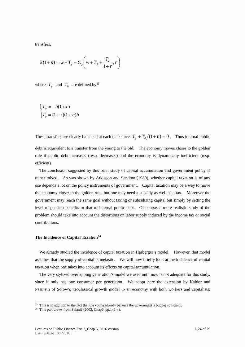
Lectures on Public Finance Part 2_Chap 5, 2016 version P.24 of 29 Last updated 19/4/2016
transfers:
+++−+=+ r
rT
TwCTwnk vjyy ,
1)1(
where yT and 0T are defined by25
++=
+−=
bnrTrbTy
)1)(1()1(
0
These transfers are clearly balanced at each date since 0)1(0 =++ nTTy . Thus internal public
debt is equivalent to a transfer from the young to the old. The economy moves closer to the golden
rule if public debt increases (resp. decreases) and the economy is dynamically inefficient (resp.
efficient).
The conclusion suggested by this brief study of capital accumulation and government policy is
rather mixed. As was shown by Atkinson and Sandmo (1980), whether capital taxation is of any
use depends a lot on the policy instruments of government. Capital taxation may be a way to move
the economy closer to the golden rule, but one may need a subsidy as well as a tax. Moreover the
government may reach the same goal without taxing or subsidizing capital but simply by setting the
level of pension benefits or that of internal public debt. Of course, a more realistic study of the
problem should take into account the distortions on labor supply induced by the income tax or social
contributions.
The Incidence of Capital Taxation26
We already studied the incidence of capital taxation in Harberger’s model. However, that model
assumes that the supply of capital is inelastic. We will now briefly look at the incidence of capital
taxation when one takes into account its effects on capital accumulation.
The very stylized overlapping generation’s model we used until now is not adequate for this study,
since it only has one consumer per generation. We adopt here the extension by Kaldor and
Pasinetti of Solow’s neoclassical growth model to an economy with both workers and capitalists.
25 This is in addition to the fact that the young already balance the government’s budget constraint. 26 This part draws from Salanié (2003, Chap6, pp.141-4).
Lectures on Public Finance Part 2_Chap 5, 2016 version P.25 of 29 Last updated 19/4/2016
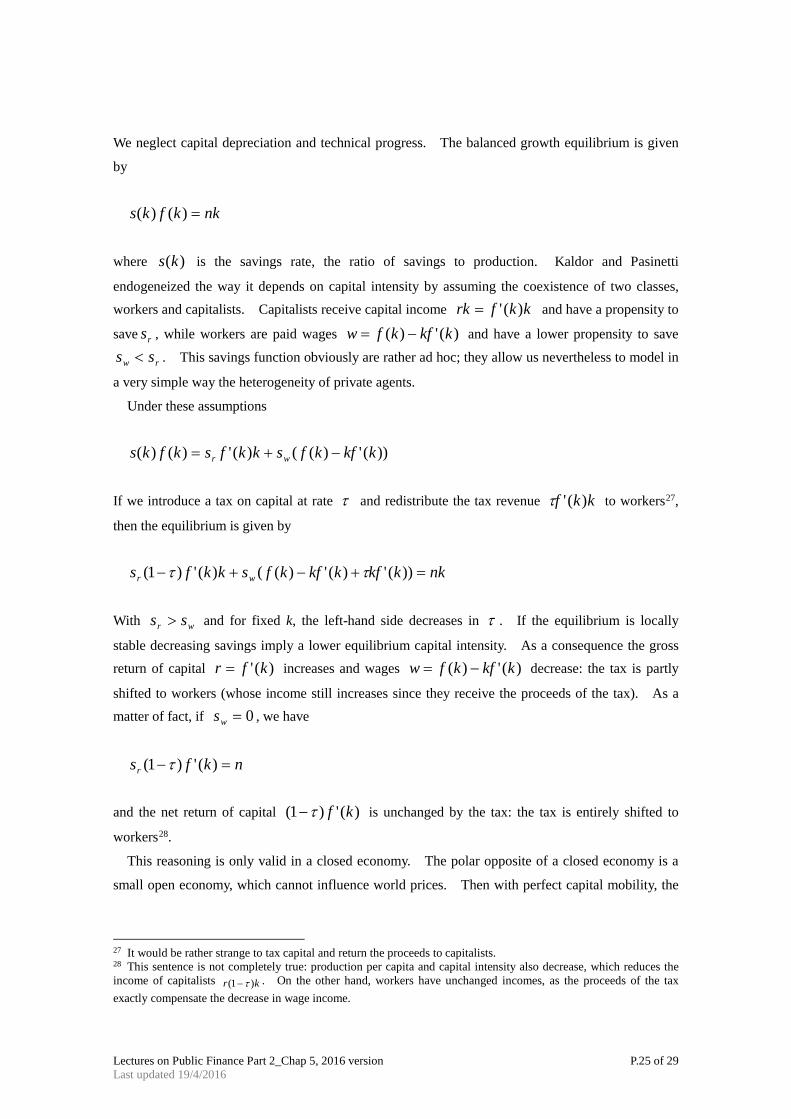
We neglect capital depreciation and technical progress. The balanced growth equilibrium is given
by
nkkfks =)()(
where )(ks is the savings rate, the ratio of savings to production. Kaldor and Pasinetti
endogeneized the way it depends on capital intensity by assuming the coexistence of two classes, workers and capitalists. Capitalists receive capital income kkfrk )('= and have a propensity to
save rs , while workers are paid wages )(')( kkfkfw −= and have a lower propensity to save
rw ss < . This savings function obviously are rather ad hoc; they allow us nevertheless to model in
a very simple way the heterogeneity of private agents.
Under these assumptions
))(')(()(')()( kkfkfskkfskfks wr −+=
If we introduce a tax on capital at rate τ and redistribute the tax revenue kkf )('τ to workers27,
then the equilibrium is given by
nkkkfkkfkfskkfs wr =+−+− ))(')(')(()(')1( ττ
With wr ss > and for fixed k, the left-hand side decreases in τ . If the equilibrium is locally
stable decreasing savings imply a lower equilibrium capital intensity. As a consequence the gross return of capital )(' kfr = increases and wages )(')( kkfkfw −= decrease: the tax is partly
shifted to workers (whose income still increases since they receive the proceeds of the tax). As a matter of fact, if 0=ws , we have
nkfsr =− )(')1( τ
and the net return of capital )(')1( kfτ− is unchanged by the tax: the tax is entirely shifted to
workers28.
This reasoning is only valid in a closed economy. The polar opposite of a closed economy is a
small open economy, which cannot influence world prices. Then with perfect capital mobility, the
27 It would be rather strange to tax capital and return the proceeds to capitalists. 28 This sentence is not completely true: production per capita and capital intensity also decrease, which reduces the income of capitalists kr )1( τ− . On the other hand, workers have unchanged incomes, as the proceeds of the tax exactly compensate the decrease in wage income.
Lectures on Public Finance Part 2_Chap 5, 2016 version P.26 of 29 Last updated 19/4/2016
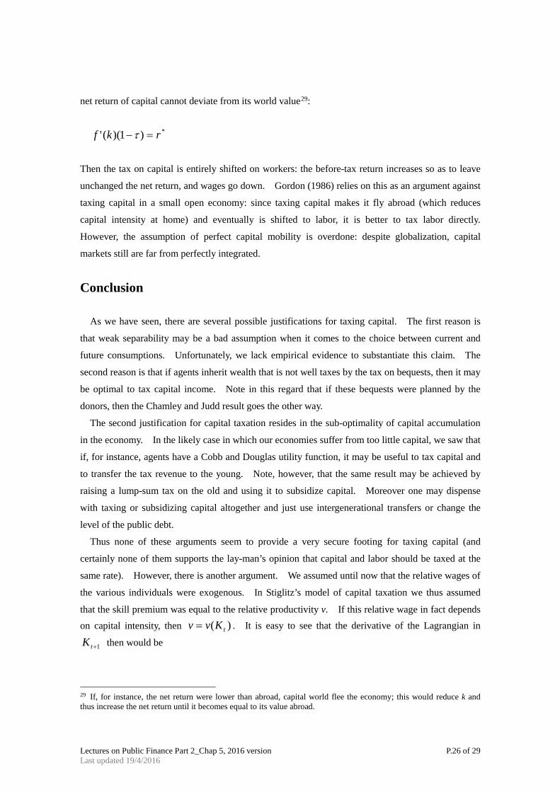
net return of capital cannot deviate from its world value29:
*)1)((' rkf =−τ
Then the tax on capital is entirely shifted on workers: the before-tax return increases so as to leave
unchanged the net return, and wages go down. Gordon (1986) relies on this as an argument against
taxing capital in a small open economy: since taxing capital makes it fly abroad (which reduces
capital intensity at home) and eventually is shifted to labor, it is better to tax labor directly.
However, the assumption of perfect capital mobility is overdone: despite globalization, capital
markets still are far from perfectly integrated.
Conclusion
As we have seen, there are several possible justifications for taxing capital. The first reason is
that weak separability may be a bad assumption when it comes to the choice between current and
future consumptions. Unfortunately, we lack empirical evidence to substantiate this claim. The
second reason is that if agents inherit wealth that is not well taxes by the tax on bequests, then it may
be optimal to tax capital income. Note in this regard that if these bequests were planned by the
donors, then the Chamley and Judd result goes the other way.
The second justification for capital taxation resides in the sub-optimality of capital accumulation
in the economy. In the likely case in which our economies suffer from too little capital, we saw that
if, for instance, agents have a Cobb and Douglas utility function, it may be useful to tax capital and
to transfer the tax revenue to the young. Note, however, that the same result may be achieved by
raising a lump-sum tax on the old and using it to subsidize capital. Moreover one may dispense
with taxing or subsidizing capital altogether and just use intergenerational transfers or change the
level of the public debt.
Thus none of these arguments seem to provide a very secure footing for taxing capital (and
certainly none of them supports the lay-man’s opinion that capital and labor should be taxed at the
same rate). However, there is another argument. We assumed until now that the relative wages of
the various individuals were exogenous. In Stiglitz’s model of capital taxation we thus assumed
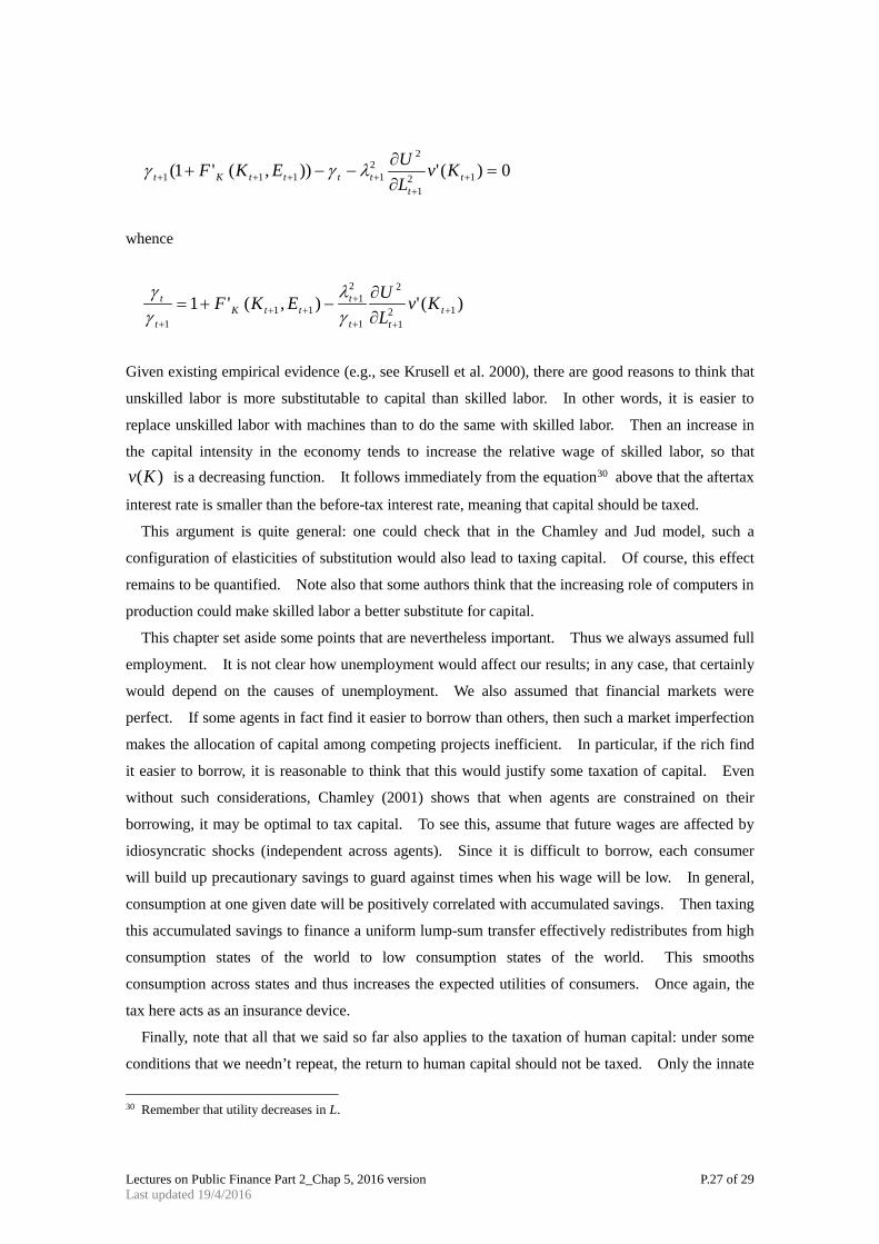
that the skill premium was equal to the relative productivity v. If this relative wage in fact depends on capital intensity, then )( tKvv = . It is easy to see that the derivative of the Lagrangian in
1+tK then would be
29 If, for instance, the net return were lower than abroad, capital world flee the economy; this would reduce k and thus increase the net return until it becomes equal to its value abroad.
Lectures on Public Finance Part 2_Chap 5, 2016 version P.27 of 29 Last updated 19/4/2016
0)(')),('1( 121
22
1111 =∂∂
−−+ ++
++++ tt
ttttKt KvLUEKF λγγ
whence
)('),('1 121
2
1
21
111
+++
+++
+ ∂∂
−+= ttt
tttK
t
t KvLUEKF
γλ
γγ
Given existing empirical evidence (e.g., see Krusell et al. 2000), there are good reasons to think that
unskilled labor is more substitutable to capital than skilled labor. In other words, it is easier to
replace unskilled labor with machines than to do the same with skilled labor. Then an increase in
the capital intensity in the economy tends to increase the relative wage of skilled labor, so that )(Kv is a decreasing function. It follows immediately from the equation30 above that the aftertax
interest rate is smaller than the before-tax interest rate, meaning that capital should be taxed.
This argument is quite general: one could check that in the Chamley and Jud model, such a
configuration of elasticities of substitution would also lead to taxing capital. Of course, this effect
remains to be quantified. Note also that some authors think that the increasing role of computers in
production could make skilled labor a better substitute for capital.
This chapter set aside some points that are nevertheless important. Thus we always assumed full
employment. It is not clear how unemployment would affect our results; in any case, that certainly
would depend on the causes of unemployment. We also assumed that financial markets were
perfect. If some agents in fact find it easier to borrow than others, then such a market imperfection
makes the allocation of capital among competing projects inefficient. In particular, if the rich find
it easier to borrow, it is reasonable to think that this would justify some taxation of capital. Even
without such considerations, Chamley (2001) shows that when agents are constrained on their
borrowing, it may be optimal to tax capital. To see this, assume that future wages are affected by
idiosyncratic shocks (independent across agents). Since it is difficult to borrow, each consumer
will build up precautionary savings to guard against times when his wage will be low. In general,
consumption at one given date will be positively correlated with accumulated savings. Then taxing
this accumulated savings to finance a uniform lump-sum transfer effectively redistributes from high
consumption states of the world to low consumption states of the world. This smooths
consumption across states and thus increases the expected utilities of consumers. Once again, the
tax here acts as an insurance device.
Finally, note that all that we said so far also applies to the taxation of human capital: under some
conditions that we needn’t repeat, the return to human capital should not be taxed. Only the innate
30 Remember that utility decreases in L.
Lectures on Public Finance Part 2_Chap 5, 2016 version P.28 of 29 Last updated 19/4/2016
productivity of agents should be taxed. This recommendation may seem abstract, but one can
derive practical consequences from it. For a start, assume that the tax on labor income is
proportional. Then a student who must decide whether to study one more year compares the value
of his forgone wages to the increase in future wages that a higher diploma will give him. With a
proportional tax, the tax rate appears on both sides a drop out so that the tax is neutral. In practice,
the tax is usually progressive and thus it discourages the accumulation of human capital. Moreover
investments in human capital are not limited to forgone wages. We should also include tuition fees,
which therefore should be deductible from taxes. Similarly taxes paid to finance public education
expenditures should be deductible from taxable income.
Lectures on Public Finance Part 2_Chap 5, 2016 version P.29 of 29 Last updated 19/4/2016
References Abel, A., G. Mankiw, L. Summers, and R. Zeckhauser (1989) “Assessing dynamic efficiency:
Theory and Evidence.” Review of Economic Studies, 56: 1-20. Arrow, K. (1970) Essays in the Theory of Risk-Bearing. North-Holland. Atkinson, A., and A. Sandmo (1980) “Welfare implications of the taxation of savings.”
Economic Journal, 90: 529-49. Auerbach, A., and L. Kotlikoff (1987) Dynamic Fiscal Policy, Cambridge University Press. Bernheim, D. (2002) “Taxation and Saving”, in Handbook of Public Economics, (eds.) A.J.
Auerback and M. Feldstein, vol.3, chap. 18, pp.1173-1249, Elsevier. Boskin, M. (1978) “Taxation, Saving, and the Rate of Interest” in Journal of Political Economy
(86) Apr. part 2. Cass D. and J. Stiglitz (1970) “The structure of investor preferences and asset returns and
separability in portfolio allocation”, Journal of Economic Theory, 2, pp.122-60. Chamley, C. (1986) “Optimal taxation of capital income in general equilibrium with infinite
lives.” Econometrica, 54: 607-22. Chamley, C. (2001) “Capital income taxation, wealth distribution and borrowing constraints.”
Journal of Public Economics, 79: 55-69. Diamond, P. (1965) “National debt in a neoclassical growth model.” American Economic
Review, 55:1126-50. Domar E. and R. Musgrave (1944) “Proportional Income Taxation and Risk-Taking”, Quarterly
Journal of Economics, 58, pp.388-422. Gordon, R. (1986) “Taxation of investment and savings in a world economy.” American
Economic Review, 76: 1086-1102. Hilman, A.L. (2003) Public Finance and Public Policy, Cambridge; Cambridge University
Press. Judd, K. (1985) “Redistributive taxation in a simple perfect foresight model.” Journal of Public
Economics, 28: 59-83. Krusell, P., L. Ohanian, J.-V. Rios-Rull, and G. Violante (2000) “Capital-skill complementarity
and inequality: A macroeconomic analysis.” Econometrica, 68: 1029-53. Mossin, J. (1968) “Taxation and Risk-taking: An Expected Utility Approach”, Economica, 137,
pp.74-82. Ordover, J., and E. Phelps (1979) “The concept of optimal taxation in the overlapping
generations model of capital and wealth.” Journal of Public Economics, 12: 1-26. Poterba J. (2002) Taxation, risk-taking, and household portfolio behavior, in Handbook of
Public Economics, (eds.) A.J. Auerback and M. Feldstein, vol.3, chap. 17, pp.1109-1171, North-Holland.
Salanié, B. (2003) The Economics of Taxation, Cambridge, MA; The MIT Press Samuelson, P. (1958) “An exact consumption-loan model of interest with or without the social
contrivance of money.” Journal of Political Economy, 66: 467-82. Stiglitz, J. (1985) “Inequality and capital taxation.” IMSSS Technical Report 457, Stanford
University. Summers, L. (1981) “Taxation and capital accumulation in a life cycle growth model.”
American Economic Review, 71: 533-54. Tobin, J. (1958) “Liquidity preference as behavior towards risk.” Review of Economic Studies,
25: 65-8.