Chapter 40. Wave Functions and UncertaintyChapter 40. Wave Functions and Uncertainty

The wave function characterizes particles in pterms of the probability of finding them at various points in space. This scanning tunneling microscope image of graphite shows the mostof graphite shows the most probable place to find electrons.electrons.

Chapter Goal: To introduce the wave‐function description pof matter and learn how it is interpreted.

Chapter Chapter 40. Wave Functions and . Wave Functions and UncertaintyUncertainty

Topics:UncertaintyUncertainty

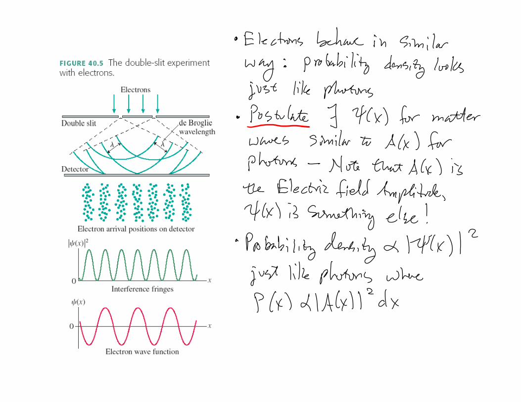
•Waves, Particles, and the Double‐Slit Experiment  

i h d h i•Connecting the Wave and Photon Views  

•The Wave Function  

•Normalization  

•Wave Packets  

•The Heisenberg Uncertainty Principle

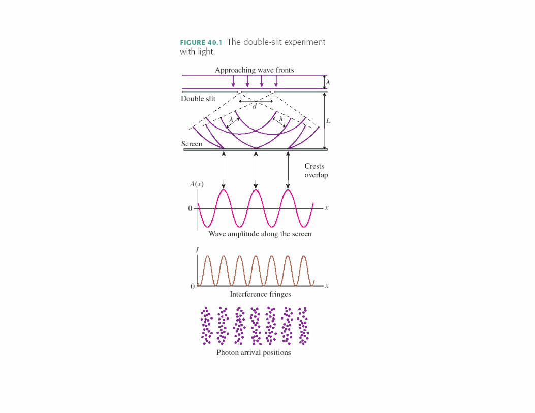
Review double slitReview double slit

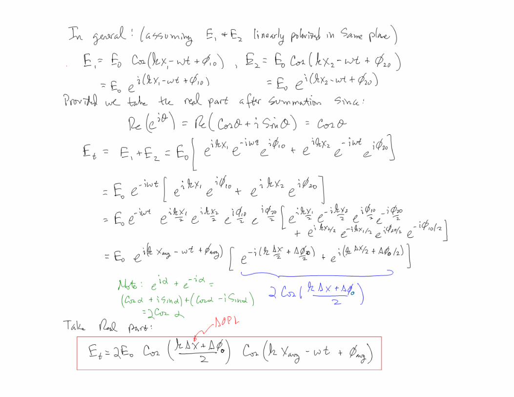
Connecting the Wave and Photon ViewsConnecting the Wave and Photon Views

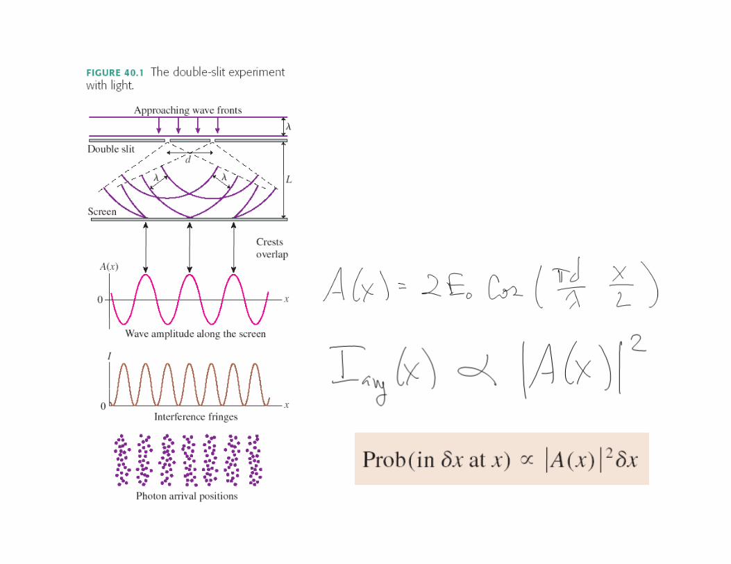
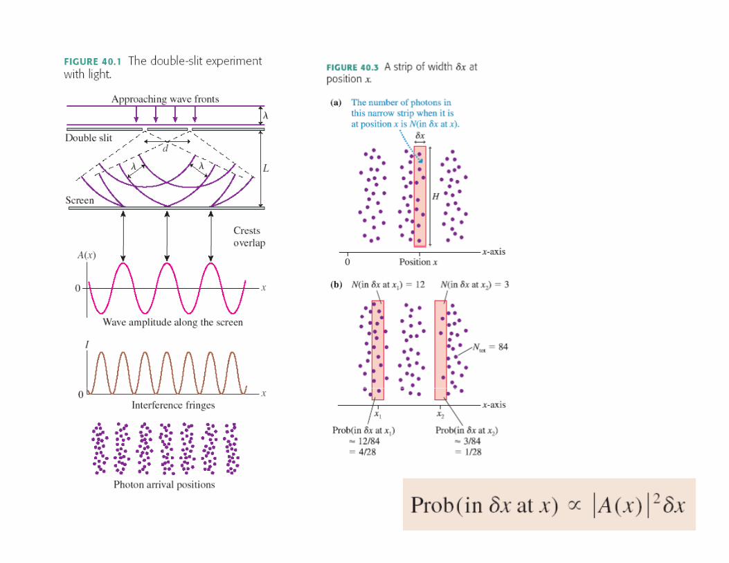
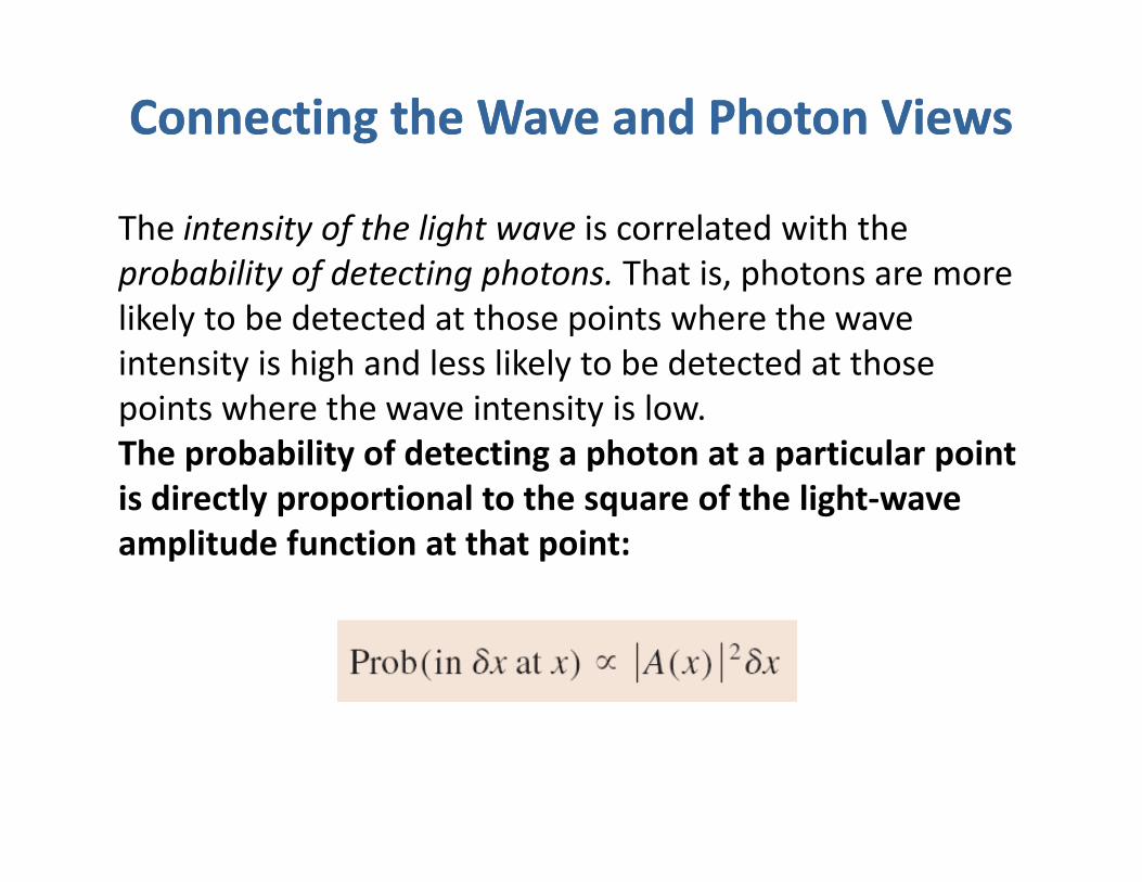
The intensity of the light wave is correlated with the probability of detecting photons That is photons are moreprobability of detecting photons. That is, photons are more likely to be detected at those points where the wave intensity is high and less likely to be detected at those points where the wave intensity is low.The probability of detecting a photon at a particular point is directly proportional to the square of the light waveis directly proportional to the square of the light‐wave amplitude function at that point:

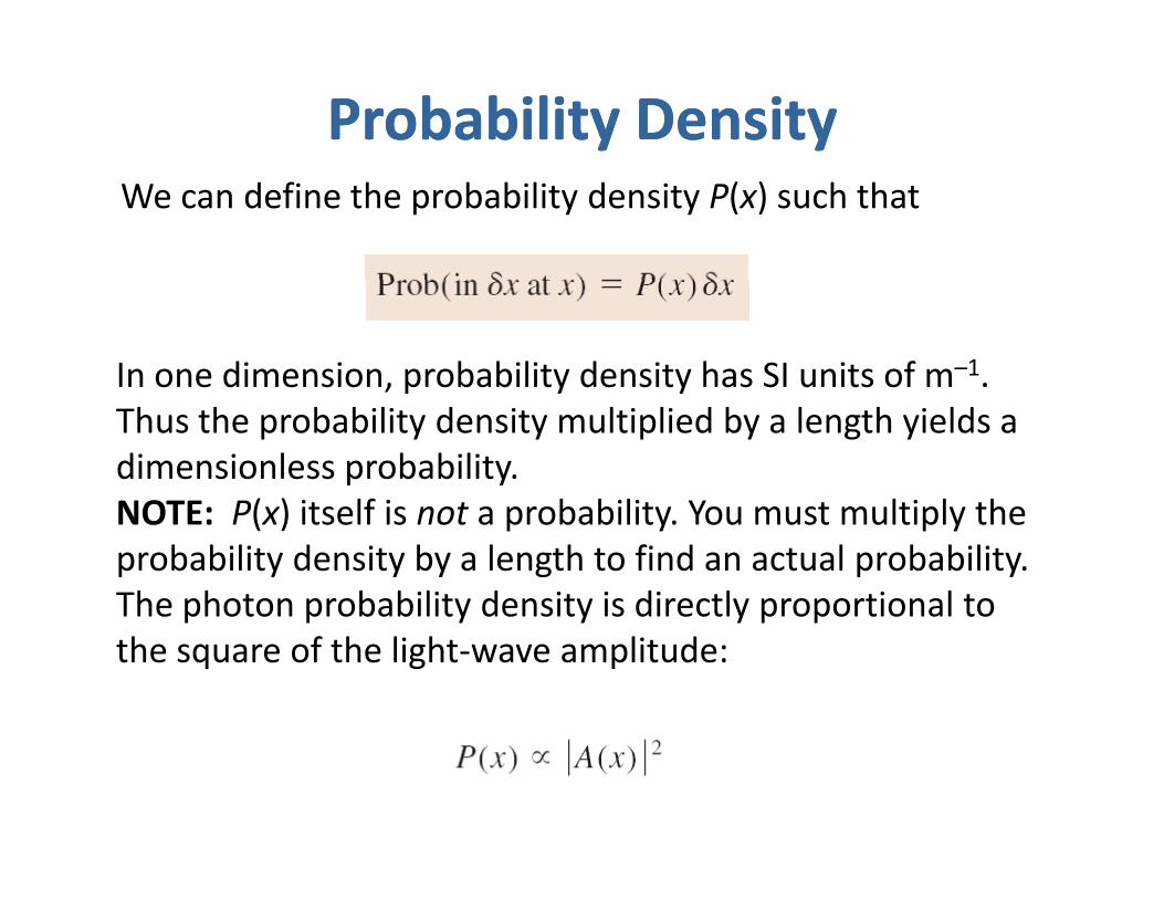
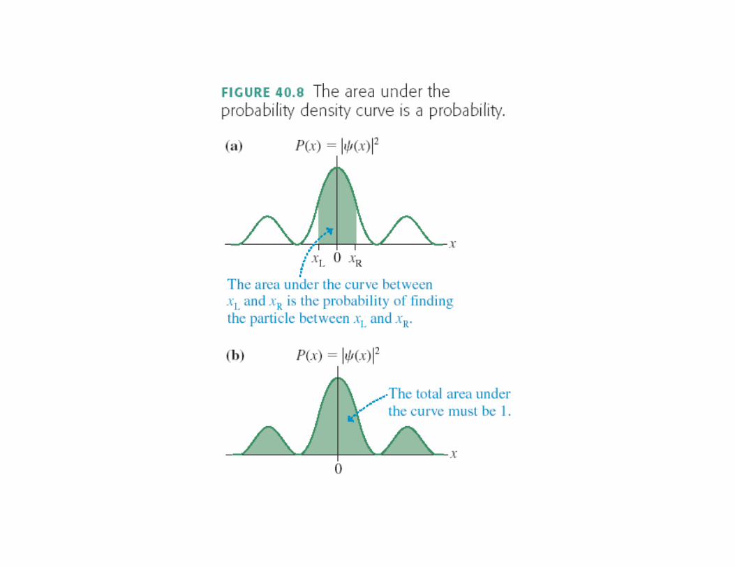
Probability DensityProbability DensityWe can define the probability density P(x) such that

In one dimension, probability density has SI units of m–1. p y yThus the probability density multiplied by a length yields a dimensionless probability.NOTE P( ) itself is not a probabilit Yo m st m ltipl theNOTE:  P(x) itself is not a probability. You must multiply the probability density by a length to find an actual probability. The photon probability density is directly proportional to p p y y y p pthe square of the light‐wave amplitude:

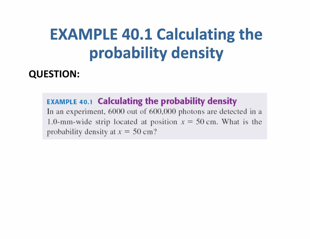
EXAMPLE 40.1 Calculating the EXAMPLE 40.1 Calculating the probability densityprobability density

QUESTION:QUESTION:

EXAMPLE 40.1 Calculating the EXAMPLE 40.1 Calculating the probability densityprobability density

NormalizationNormalizationNormalizationNormalization• A photon or electron has to land somewhere on the detector after passing through an experimentaldetector after passing through an experimental apparatus. 

• Consequently, the probability that it will be detected atConsequently, the probability that it will be detected at some position is 100%.

• The statement that the photon or electron has to land psomewhere on the x‐axis is expressed mathematically as

• Any wave function must satisfy this normalization conditioncondition.

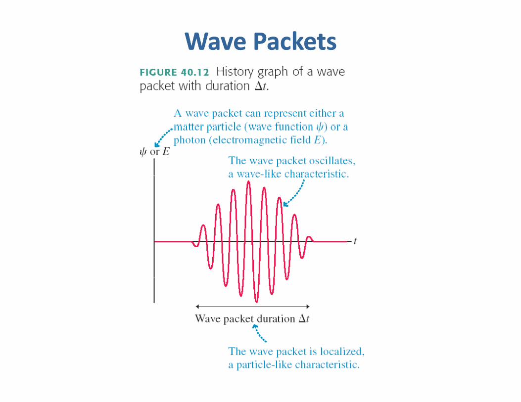
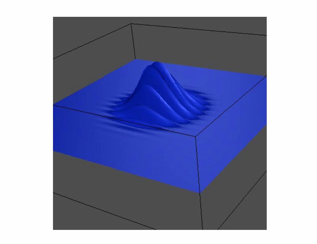
Wave PacketsWave Packets

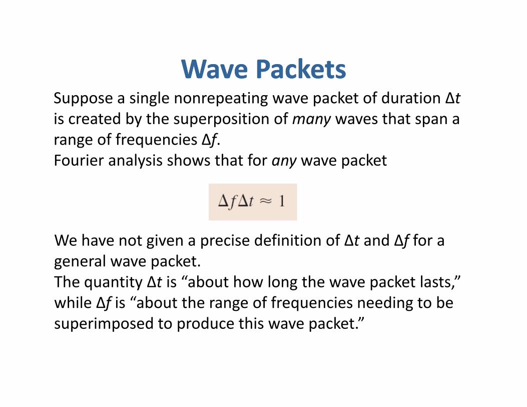
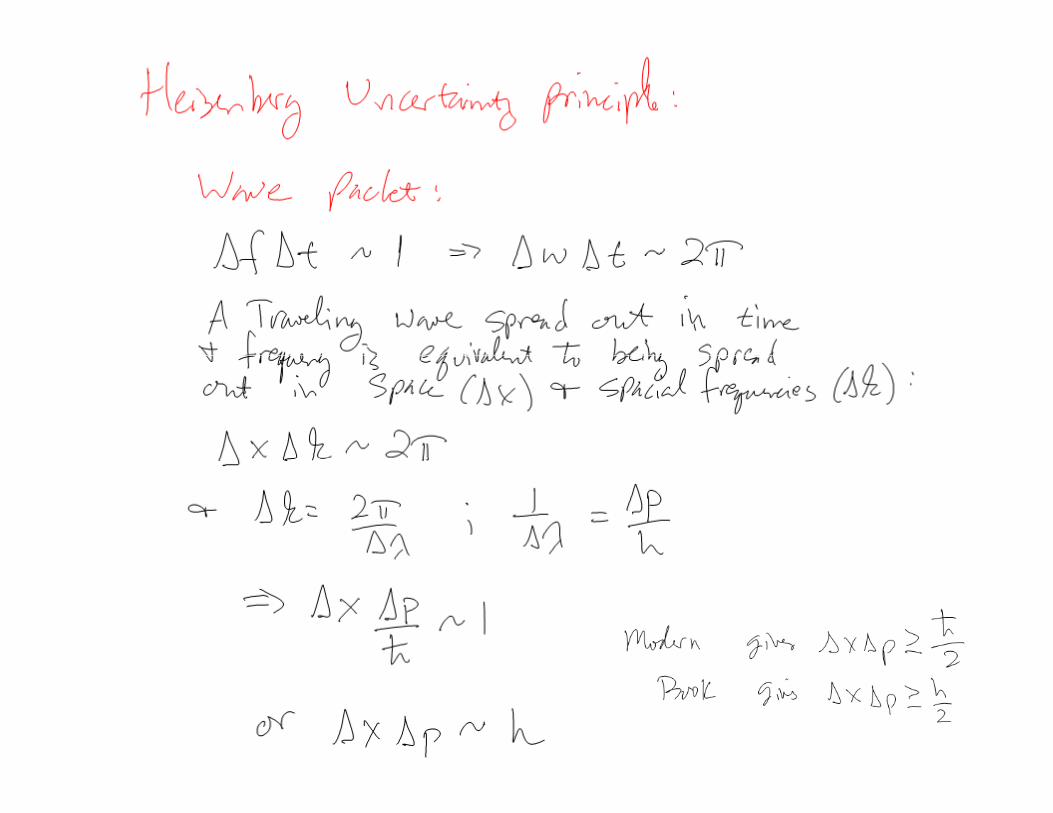
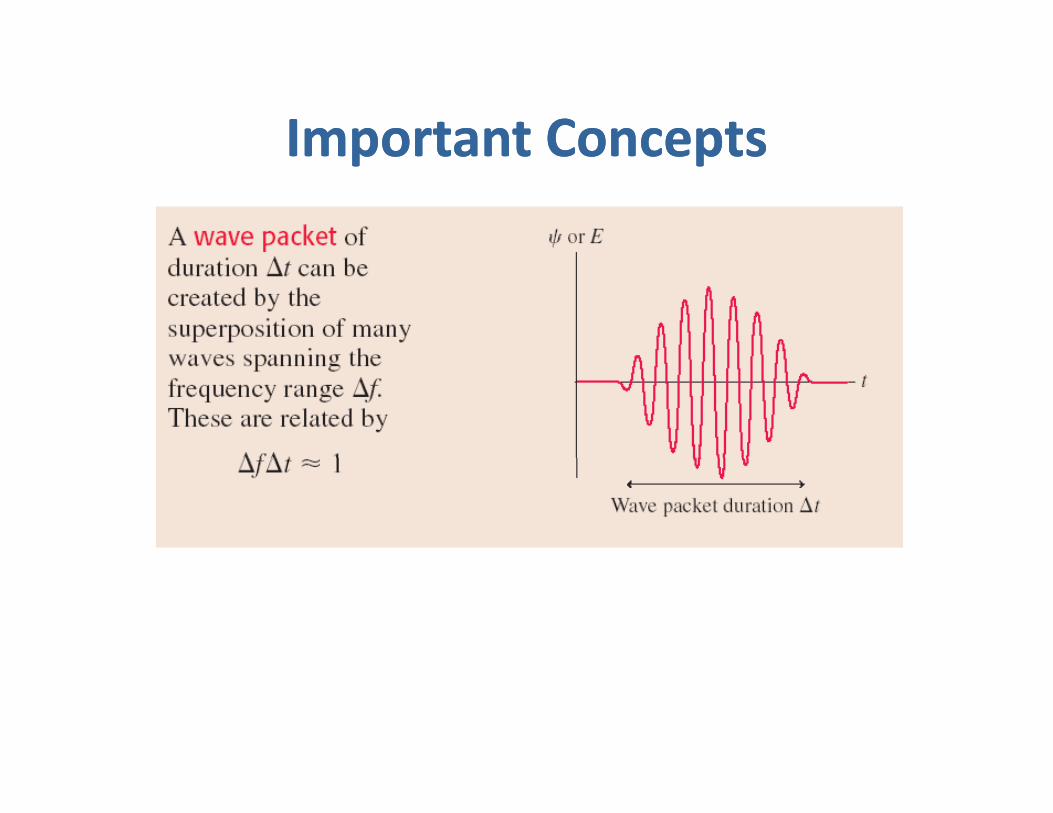
Wave PacketsWave PacketsWave PacketsWave PacketsSuppose a single nonrepeating wave packet of duration Δtis created by the superposition of many waves that span a y p p y prange of frequencies Δf. Fourier analysis shows that for any wave packet

We have not given a precise definition of Δt and Δf for a general wave packet.The quantity Δt is “about how long the wave packet lasts ”The quantity Δt is  about how long the wave packet lasts,  while Δf is “about the range of frequencies needing to be superimposed to produce this wave packet.”

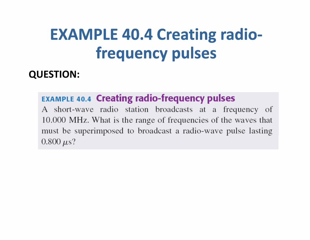
EXAMPLE 40.4 Creating radioEXAMPLE 40.4 Creating radio‐‐frequency pulsesfrequency pulses

QUESTION:QUESTION:

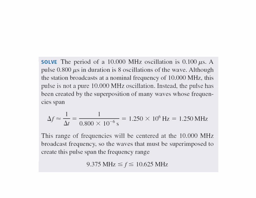
EXAMPLE 40.4 Creating radioEXAMPLE 40.4 Creating radio‐‐frequency pulsesfrequency pulses

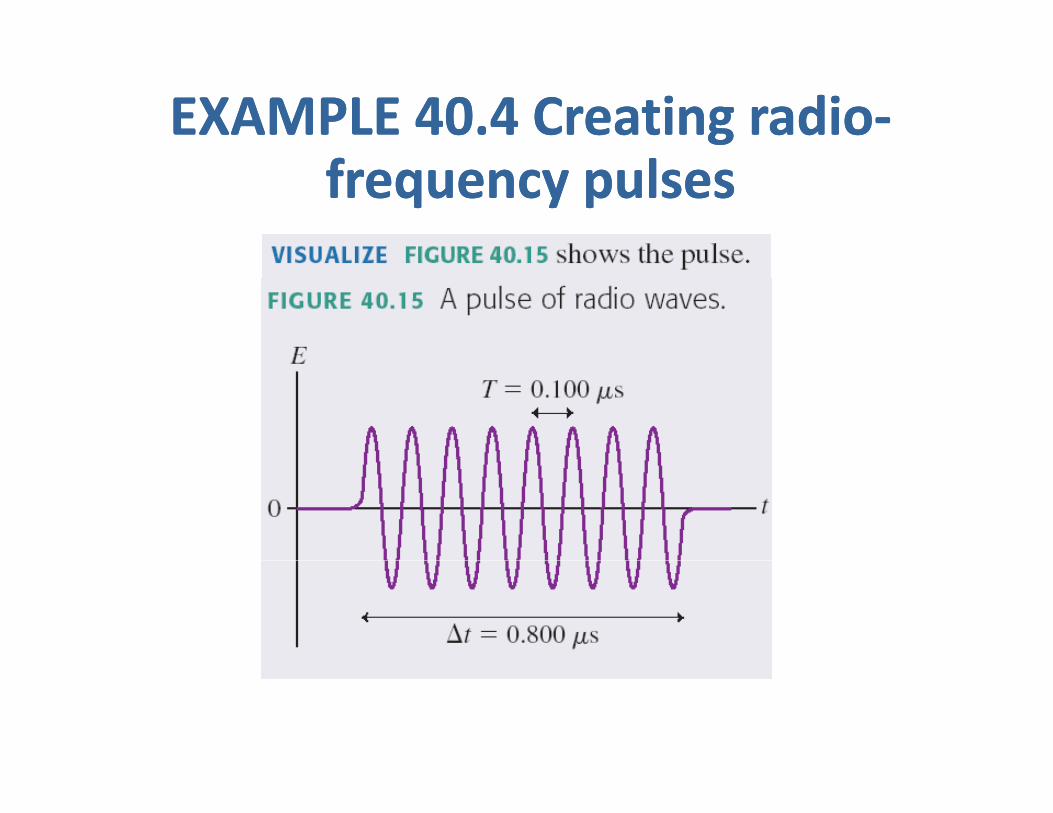
EXAMPLE 40.4 Creating radioEXAMPLE 40.4 Creating radio‐‐frequency pulsesfrequency pulses

The Heisenberg Uncertainty PrincipleThe Heisenberg Uncertainty PrincipleThe Heisenberg Uncertainty PrincipleThe Heisenberg Uncertainty Principle•The quantity Δx is the length or spatial extent of a wave packet.p

•Δpx is a small range of momenta corresponding to the small range of frequencies within the wave packet.

•Any matter wave must obey the condition

This statement about the relationship between the position and momentum of a particle was proposed by Heisenberg in 1926 Physicists often just call it theHeisenberg in 1926. Physicists often just call it the uncertainty principle.

The Heisenberg Uncertainty PrincipleThe Heisenberg Uncertainty PrincipleThe Heisenberg Uncertainty PrincipleThe Heisenberg Uncertainty Principle

•If we want to know where a particle is located, we measure its position x with uncertainty Δx.

•If we want to know how fast the particle is going, we d l l lneed to measure its velocity vx or, equivalently, its 

momentum px. This measurement also has some uncertainty Δpuncertainty Δpx.

•You cannot measure both x and px simultaneously with arbitrarily good precision.y g p

•Any measurements you make are limited by the condition that ΔxΔpx ≥ h/2.x

•Our knowledge about a particle is inherently uncertain.

General PrinciplesGeneral PrinciplesGeneral PrinciplesGeneral Principles

General PrinciplesGeneral PrinciplesGeneral PrinciplesGeneral Principles

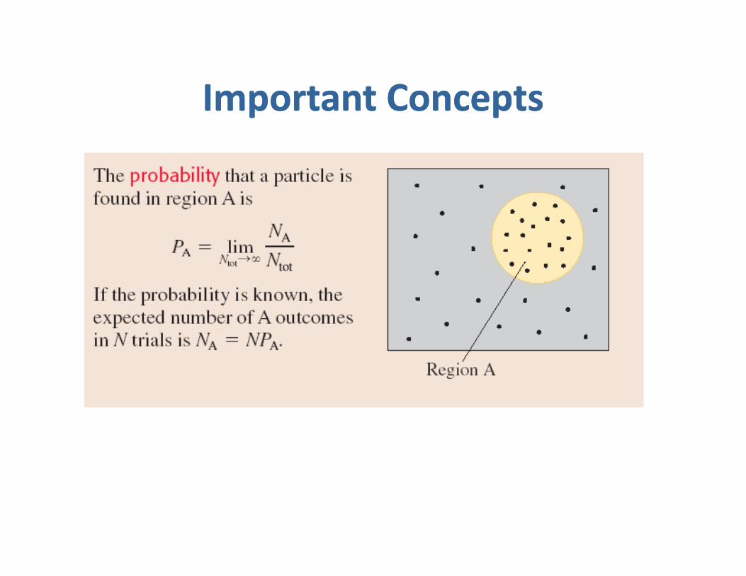
Important ConceptsImportant ConceptsImportant ConceptsImportant Concepts

Important ConceptsImportant ConceptsImportant ConceptsImportant Concepts

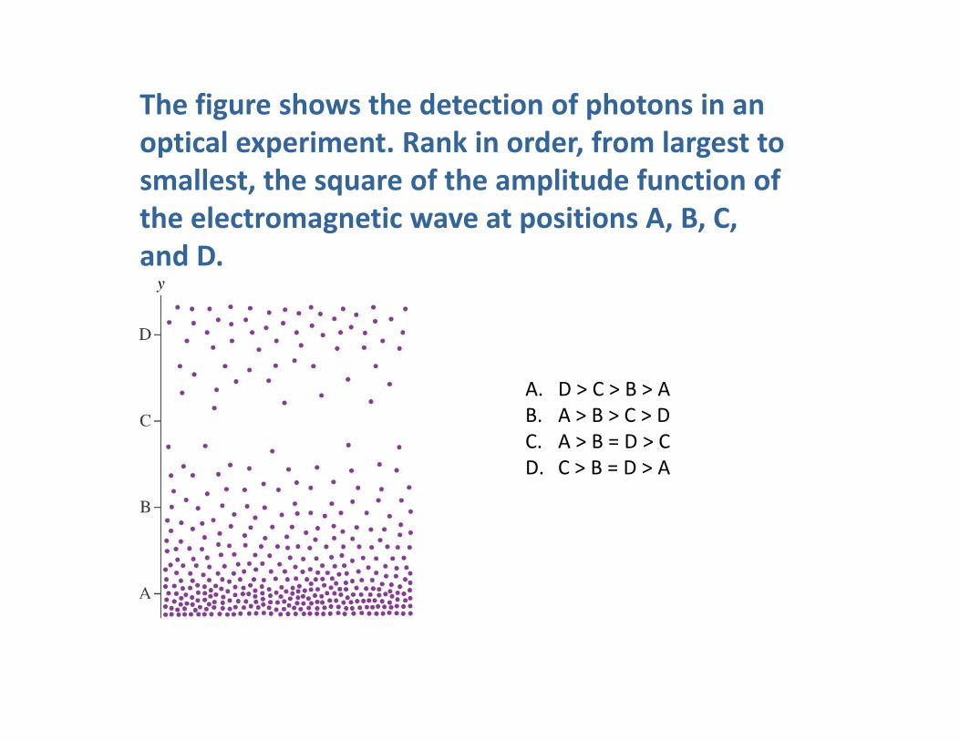
The figure shows the detection of photons in an optical e periment Rank in order from lar est tooptical experiment. Rank in order, from largest to smallest, the square of the amplitude function of the electromagnetic wave at positions A, B, C, g p , , ,and D.

A. D > C > B > A B A > B > C > DB. A > B > C > D C. A > B = D > C D. C > B = D > A 

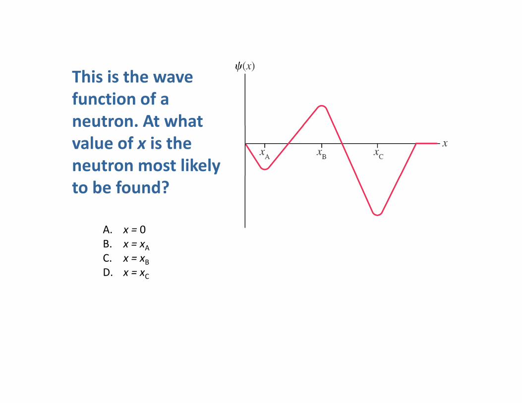
This is the waveThis is the wave function of a neutron. At whatneutron. At what value of x is the neutron most likely to be found?

A 0A. x = 0B. x = xAC. x = xBD. x = xCC

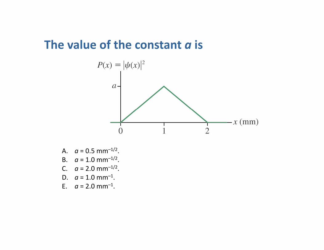
The value of the constant a isThe value of the constant a is

A. a = 0.5 mm–1/2.B. a = 1.0 mm–1/2.C. a = 2.0 mm–1/2.D. a = 1.0 mm–1.E. a = 2.0 mm–1.

What minimum bandwidth must a medium have to transmit a 100‐ns‐long pulse?

A. 100 MHzB. 0.1 MHzC. 1 MHzD. 10 MHzE. 1000 MHz