Chapter 4: The Black-Scholes Equation - Asian Scientist Magazine

AN INTRODUCTION TO COMPUTATIONAL FINANCE © Imperial College Presshttp://www.worldscibooks.com/economics/p556.html

October 22, 2008 9:41 World Scientific Book - 9in x 6in introduction

Chapter 4

The Black-Scholes Equation

The most important application of the Ito calculus, derived from the Itolemma, in financial mathematics is the pricing of options. The most famousresult in this area is the Black-Scholes formulae for pricing European vanillacall and put options. As a consequence of the formulae, both in theoreticaland practical applications, Robert Merton and Myron Scholes were awardedthe Nobel Prize for Economics in 1997 to honour their contributions tooption pricing. Unfortunately, Fischer Black, who has also given his nameand contributions, had passed away two years before.

In their famous work, in 1973, Black and Scholes transformed the op-tion pricing problem into the task of solving a (parabolic) partial differen-tial equation (PDE) with a final condition. The main conceptual idea ofBlack and Scholes lies in the construction of a riskless portfolio taking posi-tions in bonds (cash), option, and the underlying stock. Such an approachstrengthens the use of the no-arbitrage principle as well.

Derivation of a closed-form solution to the Black-Scholes equation de-pends on the fundamental solution of the heat equation. Hence, it is im-portant, at this point, to transform the Black-Scholes equation to the heatequation by change of variables. Having found the closed-form solution tothe heat equation, it is possible to transform it back to find the correspond-ing solution of the Black-Scholes PDE.

The connection between an initial and/or boundary value problem fordifferential equations, the so-called a Cauchy problem, and the computationof the expected value of a functional of a solution of an SDE is covered by theFeynman-Kac representation theorem. However, we leave it to interestedreaders, but apply the celebrated closed-form solutions to various examples.

Indeed, an important consequence of these closed-form solutions is theuse of the Greeks: the partial derivatives of the value of an option with

111



112 An Introduction to Computational Finance

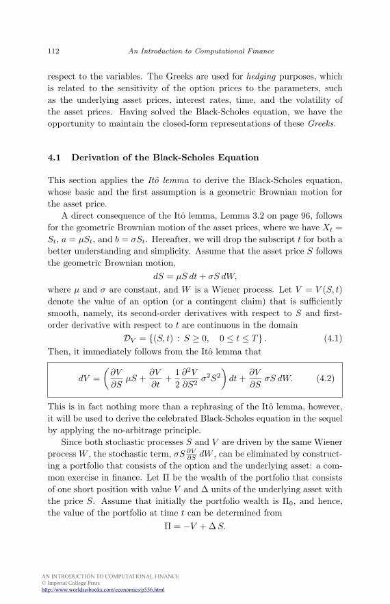
respect to the variables. The Greeks are used for hedging purposes, whichis related to the sensitivity of the option prices to the parameters, suchas the underlying asset prices, interest rates, time, and the volatility ofthe asset prices. Having solved the Black-Scholes equation, we have theopportunity to maintain the closed-form representations of these Greeks.

4.1 Derivation of the Black-Scholes Equation

This section applies the Ito lemma to derive the Black-Scholes equation,whose basic and the first assumption is a geometric Brownian motion forthe asset price.

A direct consequence of the Ito lemma, Lemma 3.2 on page 96, followsfor the geometric Brownian motion of the asset prices, where we have Xt =St, a = µSt, and b = σSt. Hereafter, we will drop the subscript t for both abetter understanding and simplicity. Assume that the asset price S followsthe geometric Brownian motion,

dS = µS dt + σS dW,

where µ and σ are constant, and W is a Wiener process. Let V = V (S, t)denote the value of an option (or a contingent claim) that is sufficientlysmooth, namely, its second-order derivatives with respect to S and first-order derivative with respect to t are continuous in the domain

DV = {(S, t) : S ≥ 0, 0 ≤ t ≤ T} . (4.1)Then, it immediately follows from the Ito lemma that

dV =(

∂V

∂SµS +

∂V

∂t+

12

∂2V

∂S2σ2S2

)dt +

∂V

∂SσS dW. (4.2)

This is in fact nothing more than a rephrasing of the Ito lemma, however,it will be used to derive the celebrated Black-Scholes equation in the sequelby applying the no-arbitrage principle.

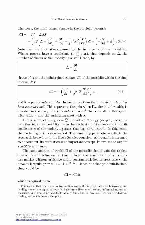
Since both stochastic processes S and V are driven by the same Wienerprocess W , the stochastic term, σS ∂V

∂S dW , can be eliminated by construct-ing a portfolio that consists of the option and the underlying asset: a com-mon exercise in finance. Let Π be the wealth of the portfolio that consistsof one short position with value V and ∆ units of the underlying asset withthe price S. Assume that initially the portfolio wealth is Π0, and hence,the value of the portfolio at time t can be determined from

Π = −V + ∆ S.



The Black-Scholes Equation 113

Therefore, the infinitesimal change in the portfolio becomes

dΠ = −dV + ∆ dS

= −(

µS

[∆− ∂V

∂S

]+

∂V

∂t+

12σ2S2 ∂2V

∂S2

)dt +

(−∂V

∂S+ ∆

)σS dW.

Note that the fluctuations caused by the increments of the underlyingWiener process have a coefficient,

(−∂V∂S + ∆

), that depends on ∆, the

number of shares of the underlying asset. Hence, by

∆ =∂V

∂S

shares of asset, the infinitesimal change dΠ of the portfolio within the timeinterval dt is

dΠ = −(

∂V

∂t+

12σ2S2 ∂2V

∂S2

)dt, (4.3)

and it is purely deterministic. Indeed, more than that: the drift rate µ hasbeen cancelled out ! This represents the gain when Π0, the initial wealth, isinvested in the risky, but frictionless market1 that consists of the optionwith value V and the underlying asset with S.

Furthermore, choosing ∆ = ∂V∂S provides a strategy (hedging) to elimi-

nate the risk in the portfolio due to the stochastic fluctuations and the driftcoefficient µ of the underlying asset that has disappeared. In this sense,the modelling of V is risk-neutral. The remaining parameter σ reflects thestochastic behaviour in the Black-Scholes equation. Although it is assumedto be constant, its estimation is an important concept, known as the impliedvolatility in finance.

The same amount of wealth Π of the portfolio should gain the risklessinterest rate in infinitesimal time. Under the assumption of a friction-less market without arbitrage and a constant risk-free interest rate r, theamount Π would grow to Π = Π0 er(t−t0). Hence, the change in infinitesimaltime would be

dΠ = rΠ dt,

which is equivalent to1This means that there are no transaction costs, the interest rates for borrowing and

lending money are equal, all parties have immediate access to any information, and allsecurities and credits are available at any time and in any size. Further, individualtrading will not influence the price.




dΠ = r (−V + ∆ S) dt

=(−rV + rS

∂V

∂S

)dt. (4.4)

This infinitesimal change dΠ in the portfolio is due to the investment inthe risk-free interest rate r, unlike the one in (4.3).

By the no-arbitrage principle and the possibility of an early exercise ofan option, it is required that the riskless gain in (4.4) cannot be more thanthe gain in the risky market given by (4.3). Hence,

−rV + rS∂V

∂S≤ −

(∂V

∂t+

12σ2S2 ∂2V

∂S2

).

Consequently, the inequality, due to Black and Scholes,

∂V

∂t+

12σ2S2 ∂2V

∂S2+ rS

∂V

∂S− rV ≤ 0 (4.5)

must hold in the domain DV . This inequality is valid no matter if the con-sidered option is European or American. Hence, an option price generallysatisfies this partial differential inequality.

If the option is assumed to be a European one, then there is no pos-sibility of early exercise, and the no-arbitrage principle implies that thesegains must be equal at the end of the infinitesimal investment time inter-val. Hence, for European options the partial differential inequality in (4.5)is reduced to the celebrated Black-Scholes equation,

∂V

∂t+

12σ2S2 ∂2V

∂S2+ rS

∂V

∂S− rV = 0 (4.6)

in the domain DV .Therefore, an option price V = V (S, t) must solve either of the inequal-

ity or the equality depending on whether the option is, respectively, Ameri-can or European. However, in (4.5) and (4.6) there is no µ, the drift rate ofthe asset. The drift rate µ has been replaced by the risk-free interest rater under the assumption of no-arbitrage. This is known as the risk-neutralvaluation principle, which is summarised in the following remark.

Remark 4.1. For pricing options the return rate µ of the underlying assetthat pays no dividend is replaced by the risk-free interest rate r. In otherwords, µ = r is assumed.




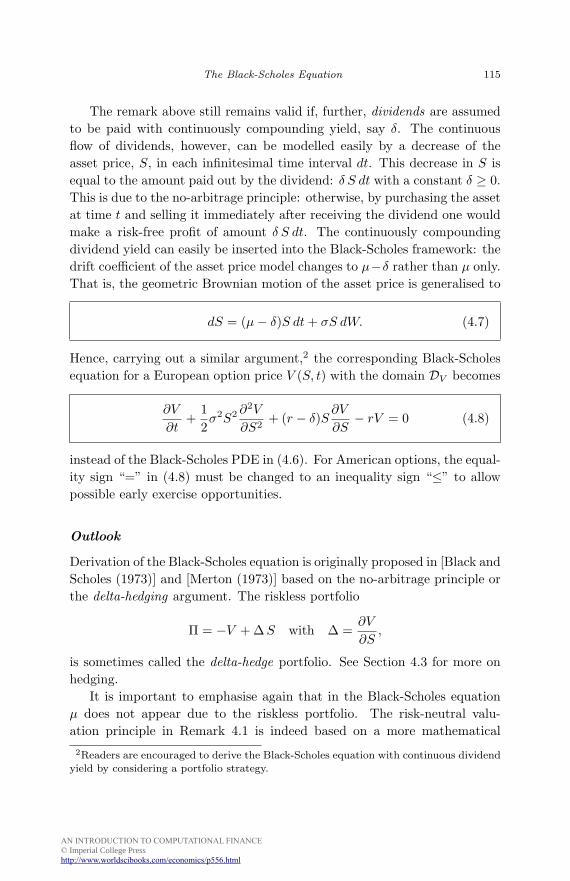
The remark above still remains valid if, further, dividends are assumedto be paid with continuously compounding yield, say δ. The continuousflow of dividends, however, can be modelled easily by a decrease of theasset price, S, in each infinitesimal time interval dt. This decrease in S isequal to the amount paid out by the dividend: δ S dt with a constant δ ≥ 0.This is due to the no-arbitrage principle: otherwise, by purchasing the assetat time t and selling it immediately after receiving the dividend one wouldmake a risk-free profit of amount δ S dt. The continuously compoundingdividend yield can easily be inserted into the Black-Scholes framework: thedrift coefficient of the asset price model changes to µ−δ rather than µ only.That is, the geometric Brownian motion of the asset price is generalised to

dS = (µ− δ)S dt + σS dW. (4.7)

Hence, carrying out a similar argument,2 the corresponding Black-Scholesequation for a European option price V (S, t) with the domain DV becomes

∂V

∂t+

12σ2S2 ∂2V

∂S2+ (r − δ)S

∂V

∂S− rV = 0 (4.8)

instead of the Black-Scholes PDE in (4.6). For American options, the equal-ity sign “=” in (4.8) must be changed to an inequality sign “≤” to allowpossible early exercise opportunities.

Outlook

Derivation of the Black-Scholes equation is originally proposed in [Black andScholes (1973)] and [Merton (1973)] based on the no-arbitrage principle orthe delta-hedging argument. The riskless portfolio

Π = −V + ∆ S with ∆ =∂V

∂S,

is sometimes called the delta-hedge portfolio. See Section 4.3 for more onhedging.

It is important to emphasise again that in the Black-Scholes equationµ does not appear due to the riskless portfolio. The risk-neutral valu-ation principle in Remark 4.1 is indeed based on a more mathematical2Readers are encouraged to derive the Black-Scholes equation with continuous dividend

yield by considering a portfolio strategy.




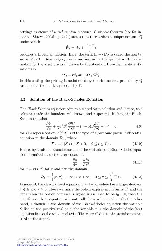
setting: existence of a risk-neutral measure. Girsanov theorem (see for in-stance (Shreve, 2004b, p. 212)) states that there exists a unique measure Qunder which

Wt = Wt +µ− r

σt

becomes a Brownian motion. Here, the term (µ− r)/σ is called the marketprice of risk . Rearranging the terms and using the geometric Brownianmotion for the asset prices St driven by the standard Brownian motion Wt,we obtain

dSt = rSt dt + σSt dWt.

In this setting the pricing is maintained by the risk-neutral probability Qrather than the market probability P.

4.2 Solution of the Black-Scholes Equation

The Black-Scholes equation admits a closed-form solution and, hence, thissolution made the founders well-known and respected. In fact, the Black-Scholes equation

∂V

∂t+

12σ2S2 ∂2V

∂S2+ (r − δ)S

∂V

∂S− rV = 0 (4.9)

for a European option V (S, t) is of the type of a parabolic partial differentialequation in the domain DV , where

DV = {(S, t) : S > 0, 0 ≤ t ≤ T} . (4.10)

Hence, by a suitable transformation of the variables the Black-Scholes equa-tion is equivalent to the heat equation,

∂u

∂τ=

∂2u

∂x2(4.11)

for u = u(x, τ) for x and t in the domain

Du ={

(x, τ) : −∞ < x < ∞, 0 ≤ τ ≤ σ2

2T

}. (4.12)

In general, the classical heat equation may be considered in a larger domain,x ∈ R and τ ≥ 0. However, since the option expires at maturity T , and thetime when the option contract is signed is assumed to be t0 = 0, then thetransformed heat equation will naturally have a bounded τ . On the otherhand, although in the domain of the Black-Scholes equation the variableS lies on the positive real axis, the variable x in the domain of the heatequation lies on the whole real axis. These are all due to the transformationsused in the sequel.




4.2.1 Transforming to the Heat Equation

Consider the transformations of the independent variables

S = K ex, and t = T − τ

σ2/2,

and the dependent variable

v(x, τ) =1K

V (S, t) =1K

V

(Kex, T − τ

σ2/2

).

In fact, the change of the independent variables ensures that the domain ofthe new dependent variable v = v(x, τ) is Du.

By the chain rule for functions of several variables, these changes ofvariables give

∂V

∂t= K

∂v

∂τ

∂τ

∂t= −σ2

2K

∂v

∂τ,

∂V

∂S= K

∂v

∂x

∂x

∂S=

K

S

∂v

∂x,

∂2V

∂S2=

∂

∂S

(∂V

∂S

)=

K

S2

(∂2v

∂x2− ∂v

∂x

).

Inserting the derivatives in the Black-Scholes equation (4.9) transforms itto a constant coefficient one:

vτ = vxx +(

r − δ

σ2/2− 1

)vx − r

σ2/2v,

where the subscripts represents the partial derivatives with respect to thecorresponding variables. Define the following new constants,

κ =r − δ

σ2/2, and ` =

δ

σ2/2,

so that the transformed PDE turns into a simpler form

vτ = vxx + (κ− 1)vx − (κ + `)v, (4.13)

the coefficients of which involve the new two constants κ and `. Thisconstant coefficient PDE must be transformed further to the heat equationby some other change of the independent variables.




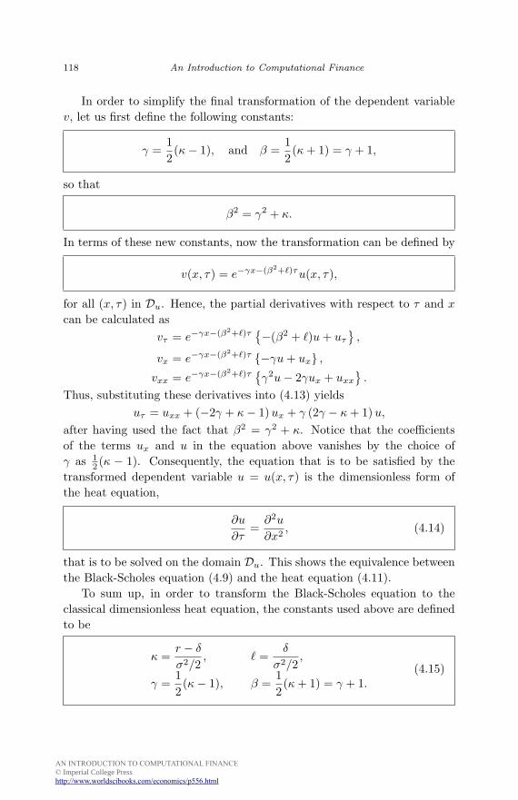
In order to simplify the final transformation of the dependent variablev, let us first define the following constants:

γ =12(κ− 1), and β =

12(κ + 1) = γ + 1,

so that

β2 = γ2 + κ.

In terms of these new constants, now the transformation can be defined by

v(x, τ) = e−γx−(β2+`)τu(x, τ),

for all (x, τ) in Du. Hence, the partial derivatives with respect to τ and x

can be calculated asvτ = e−γx−(β2+`)τ

{−(β2 + `)u + uτ

},

vx = e−γx−(β2+`)τ {−γu + ux} ,

vxx = e−γx−(β2+`)τ{γ2u− 2γux + uxx

}.

Thus, substituting these derivatives into (4.13) yieldsuτ = uxx + (−2γ + κ− 1)ux + γ (2γ − κ + 1) u,

after having used the fact that β2 = γ2 + κ. Notice that the coefficientsof the terms ux and u in the equation above vanishes by the choice ofγ as 1

2 (κ − 1). Consequently, the equation that is to be satisfied by thetransformed dependent variable u = u(x, τ) is the dimensionless form ofthe heat equation,

∂u

∂τ=

∂2u

∂x2, (4.14)

that is to be solved on the domain Du. This shows the equivalence betweenthe Black-Scholes equation (4.9) and the heat equation (4.11).

To sum up, in order to transform the Black-Scholes equation to theclassical dimensionless heat equation, the constants used above are definedto be

κ =r − δ

σ2/2, ` =

δ

σ2/2,

γ =12(κ− 1), β =

12(κ + 1) = γ + 1.

(4.15)




On the other hand, the transformations of the dependent and the indepen-dent variables that use those constants are given by

S = K ex, t = T − τ

σ2/2,

V (S, t) = K v(x, τ), v(x, τ) = e−γx−(β2+`)τ u(x, τ).(4.16)

Under these changes of variables, the domain DV is mapped to Du.The fundamental solution of the dimensionless heat equation uτ = uxx

is given by

G(x, τ) =1√4πτ

exp{−x2

4τ

}(4.17)

which satisfies the equation for all τ > 0 and x ∈ R. This can beeasily shown by direct substitution into the equation. Note also thatG(x, τ) = φ0,

√2τ (x), that is, it is the probability density function of the

normal distribution with mean zero and variance 2τ .Moreover, for a given initial condition,

u(x, 0) = u0(x), −∞ < x < ∞, (4.18)

at τ = 0, the solution of the heat equation can be written as a convolutionintegral of G and u0 as

u(x, τ) =∫ ∞

−∞G(x− ξ, τ) u0(ξ) dξ (4.19)

for τ > 0. With this representation, the function G(x− ξ, τ) is also calledthe Green’s function for the diffusion equation. It is not too difficult to showthat u = u(x, τ) represented by the convolution integral above is indeed asolution of the heat equation and satisfies

limτ→0+

u(x, τ) = u0(x).

We leave these details to the readers.Consequently, the solution of the heat equation which satisfies the initial

condition (4.18) can be represented by (4.19) or, using (4.17), by

u(x, τ) =1√4πτ

∫ ∞

−∞e−

(x−ξ)2

4τ u0(ξ) dξ. (4.20)

Therefore, in order to solve the Black-Scholes equation we need to de-termine what the initial function u0(x) = u(x, 0) corresponds to in the




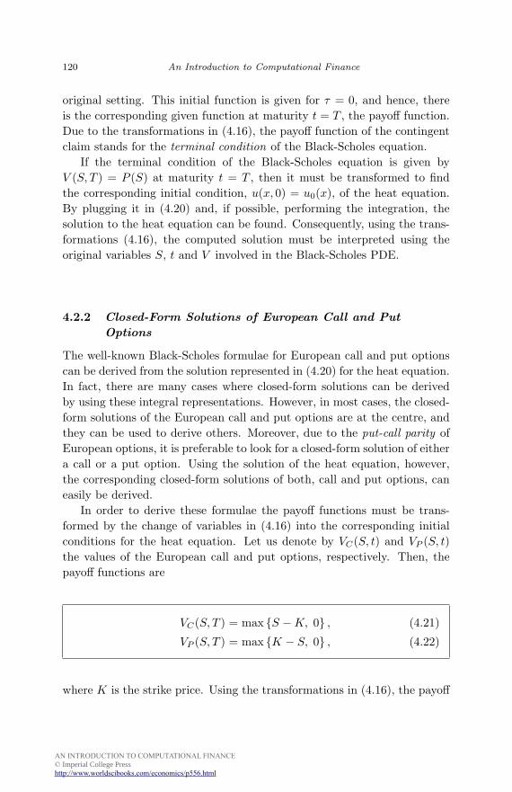
original setting. This initial function is given for τ = 0, and hence, thereis the corresponding given function at maturity t = T , the payoff function.Due to the transformations in (4.16), the payoff function of the contingentclaim stands for the terminal condition of the Black-Scholes equation.

If the terminal condition of the Black-Scholes equation is given byV (S, T ) = P (S) at maturity t = T , then it must be transformed to findthe corresponding initial condition, u(x, 0) = u0(x), of the heat equation.By plugging it in (4.20) and, if possible, performing the integration, thesolution to the heat equation can be found. Consequently, using the trans-formations (4.16), the computed solution must be interpreted using theoriginal variables S, t and V involved in the Black-Scholes PDE.

4.2.2 Closed-Form Solutions of European Call and Put

Options

The well-known Black-Scholes formulae for European call and put optionscan be derived from the solution represented in (4.20) for the heat equation.In fact, there are many cases where closed-form solutions can be derivedby using these integral representations. However, in most cases, the closed-form solutions of the European call and put options are at the centre, andthey can be used to derive others. Moreover, due to the put-call parity ofEuropean options, it is preferable to look for a closed-form solution of eithera call or a put option. Using the solution of the heat equation, however,the corresponding closed-form solutions of both, call and put options, caneasily be derived.

In order to derive these formulae the payoff functions must be trans-formed by the change of variables in (4.16) into the corresponding initialconditions for the heat equation. Let us denote by VC(S, t) and VP (S, t)the values of the European call and put options, respectively. Then, thepayoff functions are

VC(S, T ) = max {S −K, 0} , (4.21)

VP (S, T ) = max {K − S, 0} , (4.22)

where K is the strike price. Using the transformations in (4.16), the payoff




of a call option, for instance, is easily converted to

uC(x, 0) =1K

eγxVC(Kex, T )

=1K

eγx max {Kex −K, 0}

= max{

e(γ+1)x − eγx, 0}

.

Similar calculations can be carried out for the payoff function of a putoption. Using the constant β = γ + 1 in (4.15), the corresponding initialconditions at τ = 0 for the heat equation become

uC(x, 0) = max{eβx − eγx, 0

}, (4.23)

uP (x, 0) = max{eγx − eβx, 0

}. (4.24)

Substitution of these functions into the integral solution in (4.20) willthen yield the solution u = u(x, τ) for the transformed dependent variable.For example, substituting the initial condition (4.23) for a European calloption into the solution formula gives

uC(x, τ) =1√4πτ

∫ ∞

−∞e−

(x−ξ)2

4τ max{eβx − eγx, 0

}dξ

=1√4πτ

∫ ∞

0

e−(x−ξ)2

4τ

(eβx − eγx

)dξ

= Iβ − Iγ , (4.25)

where the last integrals are defined by

Iα =1√4πτ

∫ ∞

0

e−(x−ξ)2

4τ +αξ dξ (4.26)

for each α = β, γ. Calculation, or simplification of the integral Iα canfurther be carried out by a change of variables as follows:

Iα =1√4πτ

∫ ∞

0

e−[(x+2τα)−ξ]2

4τ +αξ eαx+α2τ dξ

= eαx+α2τ

∫ x+2τα√2π

−∞

1√2π

e−η2/2 dη,

where the change of variable η = x+2τα−ξ√2π

is used. Note that the lastintegral contains the probability density function of the standard normaldistribution. Hence, using the distribution function Φ,

Φ(ζ) =∫ ζ

−∞φ(η) dη =

1√2π

∫ ζ

−∞e−η2/2 dη, (4.27)




of the normal distribution with mean zero and variance one, the integralIα can be written in closed-form as

Iα = eαx+α2τ Φ(

x + 2τα√2π

). (4.28)

Therefore, the solution uC(x, τ) represented by the difference of twointegrals, as in (4.25), is simplified to

uC(x, τ) = eβx+β2τ Φ(

x + 2τβ√2π

)− eγx+γ2τ Φ

(x + 2τγ√

2π

). (4.29)

Similar calculations carried out for the transformed initial conditionuP (x, 0) in (4.24) for the put option shows that

uP (x, τ) = eγx+γ2τ Φ(−x + 2τγ√

2π

)− eβx+β2τ Φ

(−x + 2τβ√

2π

). (4.30)

What remains only is that the solutions represented by equations (4.29)and (4.30) must be transformed back in order to write the solutions of theBlack-Scholes equation for the European call and put options, respectively.This can be done by using the transformations defined by (4.16) that areaccompanied with the notations in (4.15). Let us define

d1 =x + 2τβ√

2π, and d2 =

x + 2τγ√2π

. (4.31)

Then, in terms of the original variables S = Kex and t = T − τσ2/2 of the

Black-Scholes equation, d1 and d2 can easily be obtained as

d1 =log(S/K) +

(r − δ + 1

2σ2)(T − t)

σ√

T − t, (4.32)

d2 =log(S/K) +

(r − δ − 1

2σ2)(T − t)

σ√

T − t. (4.33)

Recall that the constants β and γ were defined by (4.15). For ease ofreference, they were

γ =12(κ− 1), and β =

12(κ + 1) = γ + 1,

where κ = r−δσ2/2 . Note also that d2 can be defined via d1 as




d2 = d1 − σ√

T − t. (4.34)

On the other hand, the transformation used for the dependent variableV (S, t), the value of an option, was

V (S, t) = K v(x, t), v(x, τ) = e−γx−(β2+`)τ u(x, τ),

where ` = δσ2/2 . Hence, the value of a European call option can be converted

back from (4.29) as

VC(x, t) = Ke−γx−(β2+`)τ{

eβx+β2τ Φ(d1)− eγx+γ2τ Φ(d2)}

= Ke(β−γ)x−`τΦ(d1)−Ke(γ2−β2−`)τΦ(d2).

Here, notice that

β − γ = 1 and `τ = δ(T − t)

so that Ke(β−γ)x−`τ = Se−δ(T−t). Moreover,

(γ2 − β2 − `)τ = −(` + κ)τ = −r(T − t),

hence, Ke(γ2−β2−`)τ = Ke−r(T−t). Therefore, replacing the values of theparameters and the independent variables x and τ with the original ones,S and t, gives

VC(S, t) = Se−δ(T−t)Φ(d1)−Ke−r(T−t)Φ(d2), (4.35)

which is the celebrated Black-Scholes formula for a European call option.Similar calculations show that the value of a European put option

VP (S, t) can be written as

VP (S, t) = Ke−r(T−t)Φ(−d2)− Se−δ(T−t)Φ(−d1). (4.36)

On the other hand, this closed-form formula for the value of a Europeanput option can also be obtained from the put-call parity

VP (S, t) = VC(S, t)− Se−δ(T−t) + Ke−r(T−t) (4.37)

by using the relation Φ(−ζ) = 1−Φ(ζ), which can be proved easily, and isleft as an exercise.

Exercise 4.1. Using the definition of Φ show that

Φ(−ζ) = 1− Φ(ζ) (4.38)

holds for all ζ ∈ R.




Exercise 4.2. Show that the closed-form solution Vcon(S, t) of a cash-or-nothing option is given by

Vcon(S, t) = B e−r(T−t) Φ(d2).

A cash-or-nothing option has the payoff function

Vcon(S, T ) ={

B if S > K,

0 if S ≤ K.

That is, the reward B is paid if the asset price is more than the bet K atmaturity T .

Exercise 4.3. Show that the value V (S, t) of a European option can beexpressed as the discounted, expectation of the payoff V (S, T ) under therisk-neutrality condition: µ = r. In other words, show that

V (S, t) = e−r(T−t)EQ [V (S, T )]

= e−r(T−t)

∫ ∞

0

V (s, T ) p(s; T, S, t) ds,

where p = p(s; T, S, t) is the density function of a lognormal distribution,and it is defined by

p(s;T, S, t) =1

sσ√

2π(T − t)e− [log(s/S)−(r−δ− 1

2 σ2)(T−t)]22σ2(T−t) .

This is sometimes called the transition probability density.

Although the formulae (4.35) and (4.36) are the closed-form solutionsof the Black-Scholes equation for European call and put options, respec-tively, they still require evaluation of improper integrals. This can be done,however, numerically, in most cases. Hence, truncation of the domains ofthe integrals is unavoidable for numerical calculations.

Fortunately, a numerous numerical software includes libraries to calcu-late the error function, which is denoted by erf, and is defined by

erf(x) =2√π

∫ x

0

e−t2 dt. (4.39)

In fact, this error function is rather similar to the distribution function ofthe standard normal distribution. It is easy to write the latter in terms of




the former. For,

Φ(x) =1√2π

∫ x

−∞e−

12 ξ2

dξ =1√π

∫ x/√

2

−∞e−t2 dt

=1√π

(∫ 0

−∞e−t2 dt +

∫ x/√

2

0

e−t2 dt

).

By using the well-known integral∫ ∞

−∞e−t2 dt =

√π,

as well as the definition (4.39) of the error function, it follows that

Φ(x) =12

{1 + erf

(x/√

2)}

. (4.40)

In most cases, since the error function is available in Matlab, calculationof the value Φ(x) at x will be done by using (4.40). However, there isno explicit form for the calculation of neither Φ(x) nor erf(x), but thereare some well-known approximations collected in [Abramowitz and Stegun(1972)]. The algorithm given in the exercise below is frequently used andrelatively fast besides its accuracy. The implementation of the algorithm isleft to the readers.

Exercise 4.4. Write a program that computes the value of the standardnormal distribution function Φ(x) at a given point x. First, by using (4.40)if possible. Second, by using the following procedure.

(1) Let γ = 0.2316419.

(2) Calculate z =1

1 + γx, for x ≥ 0.

(3) Let the coefficients be

a1 = 0.319381530, a2 = −0.356563782, a3 = 1.781477937,

a4 = −1.821255978, a5 = 1.330274429.

(4) Then, the approximate value of Φ(x) for x ≥ 0 is

Φ(x) ≈ 1− φ(x) z ((((a5z + a4)z + a3)z + a2)z + a1),

where φ(x) is the value of the density function at x. If x < 0, thenapply Φ(x) = 1− Φ(−x).




Outlook

Within a more general mathematical setting, the risk-neutral expected dis-counted payoff is linked to the solution of the Black-Scholes equation by theFeynman-Kac theorem. To see this close relation we refer to (Shreve, 2004b,pp. 268–272). For an intuitive and well-illustrated introduction to the rela-tion between partial differential equations and stochastic processes, [Neftci(2000)] seems to be a good reference.

A clear and concise reference for the heat equation and its qualitativeproperties we refer to [John (1991)], which also includes the Green’s func-tions, fundamental solutions, and Fourier transforms.

For similar transformations applied to the Black-Scholes equation inorder to get the classical heat equation, readers can refer to [Barraquandand Pudet (1996); Seydel (2002); Wilmott et al. (1995)]. In this section,we skipped the transformations of the boundary conditions for options inorder to avoid some technical definitions for function spaces in which thesolutions are sought. However, readers may have a glance on the literaturereferenced above, or Chapter 6 in advance, for detailed discussions on somespecific options; preferably, European call and put options.

4.3 Hedging Portfolios: The Greeks

This section briefly considers the sensitivity of option price to the under-lying parameters, such as asset prices, volatility, interest rates, and so on.Changes in the values of these parameters will certainly change values of theoptions considerably. A portfolio consisting of options is liable to changesof these parameters and, thus, should be hedged, and the risk it is exposedto should be reduced.

Recall that the portfolio

Π = −V + ∆ S (4.41)

was considered in Section 4.1 when deriving the Black-Scholes PDE. Thisportfolio was made riskless, in other words, it did not change its value bythe stochastic fluctuations caused by the asset prices. This was achievedby choosing a ∆ number of shares from the underlying asset as

∆ =∂V

∂S. (4.42)

However, mathematically, this corresponds to the rate of change of theoption value due to the changes of the underlying asset prices. It is a




measure of the sensitivity of an option price to the asset prices, which iscalled by the Greek name: the delta of the option.

The delta of an option is particularly important in hedging portfolios.For instance, an investor likes to have a portfolio that is not affected bythe changes in the asset prices. That is, he wishes to manage a portfolio Πwhose rate of change

∆Π =∂Π∂S

(4.43)

with respect to asset prices S is zero: ∆Π = 0. This is called the delta-hedging of the portfolio.

Suppose that you are in a short position in an option with the value V ,and you want to protect yourself by taking positions in the asset becauseof the changes of the underlying asset prices S. Then, you would constructthe portfolio in (4.41), where the ∆ represents the number of shares of theasset that you need to purchase. Thus, in order to hedge the portfolio withrespect to the changes of the prices, you would require the delta of theportfolio to vanish. That is,

0 =∂Π∂S

= −∂V

∂S+ ∆.

However, this leads to the same ∆ defined in (4.42), the delta of the optionin the portfolio.

A portfolio that has to be hedged may contain several parameters, evenif it has only a single option. Of course, a portfolio may have many otherfinancial derivatives and, hence, completely different parameters than thatof an option. However, the sensitivities of a portfolio to the parametersof an option are particularly important in hedging. These sensitivities arenamed after Greek names, and simply called the Greeks of a portfolio. TheGreeks for a portfolio Π are defined as

Delta: ∆Π =∂Π∂S

, Gamma: ΓΠ =∂2Π∂S2

, Theta: ΘΠ =∂Π∂t

,

Vega: VΠ =∂Π∂σ

, Rho: ρΠ =∂Π∂r

.

Remark 4.2. Sometimes, the Greek theta, ΘΠ, of a portfolio Π is definedto be

ΘΠ =∂Π∂τm

,




where τm = T − t is the time to maturity. It is easy to use the chain ruleand obtain the relation,

∂Π∂t

=∂Π∂τm

∂τm

∂t= − ∂Π

∂τm.

Depending on his preferences, an investor may wish to hedge a port-folio that is liable to the changes in any, or several of the parameters.Thus, knowing the Greeks for the options is particularly important. Thanksto the closed-form solutions of the Black-Scholes equation. By using theclosed-form solutions, it is possible to derive the corresponding closed-formrepresentations for the Greeks of the European call and put options.

In fact, due to the put-call parity (4.37) for European options it issufficient to know the Greeks only for call options in closed-form. Thecorresponding Greeks for put options can then be derived by using theput-call parity. The Black-Scholes closed-form solution for a European calloption has been given in (4.35). For ease of reference, it is

VC(S, t) = Se−δ(T−t)Φ(d1)−Ke−r(T−t)Φ(d2), (4.44)

where Φ is the distribution function of the standard normal distributionwhose density is Φ′ = φ. Differentiating VC with respect to S gives thedelta Greek for the call option, which we will denote it by ∆C , and

∆C =∂VC

∂S= e−δ(T−t)Φ(d1) + Se−δ(T−t)φ(d1)

∂d1

∂S

−Ke−r(T−t)φ(d2)∂d2

∂S.

The partial derivatives of d1 and d2 can be easily calculated by using theirdefinitions in (4.32) and (4.33), respectively, and noticing the relation

d2 = d1 − σ√

T − t

in (4.34). Thus,

∂d1

∂S=

∂d2

∂S=

1Sσ√

T − t.

The delta ∆C of a call option can further be simplified by the use of thefollowing fact:

Se−δ(T−t)φ(d1)−Ke−r(T−t)φ(d2) = 0. (4.45)




This can be proved by considering the relation,

log(

Se−δ(T−t)φ(d1)Ke−r(T−t)φ(d2)

)= log (S/K)+(r−δ)(T − t)+log

(φ(d1)φ(d2)

)(4.46)

and the definition of the probability density function which is

φ(ξ) =1√2π

e−ξ2/2.

First, note that the last logarithm in (4.46) is simplified to

log(

φ(d1)φ(d2)

)= −1

2(d21 − d2

2

)

by use of the definition of φ. Second, the difference d21− d2

2 may be writtenas

d21 − d2

2 = 2d1σ√

T − t− σ2(T − t)

= 2 log (S/K) + 2(r − δ)(T − t)

by using (4.32) and (4.34). Therefore, (4.46) is simplified as

log(

φ(d1)φ(d2)

)= − log (S/K)− (r − δ)(T − t).

Plugging the last expression into (4.46) proves the relation,

log(

Se−δ(T−t)φ(d1)Ke−r(T−t)φ(d2)

)= 0,

which is equivalent to (4.45).Hence, summarising the calculations above shows that the delta ∆C of

a European call option is simply

∆C =∂VC

∂S= e−δ(T−t)Φ(d1). (4.47)

Note also that as τm = T−t approaches zero, d1 and d2 defined, respectively,by (4.32) and (4.33) are unbounded from above (tend to ∞) for S > K.Similarly, when S < K, they are unbounded from below (tend to −∞) asτm = T − t approaches zero. Therefore, from (4.47) it follows that the deltaof a call option has the limits:

∆C −→{

1, if S > K

0, if S < Kas τm = T − t → 0. (4.48)




On the other hand, from the put-call parity (4.37) of European options,it is easy to calculate the corresponding delta Greek ∆P for the put option.Differentiating both sides of the parity,

VP (S, t) = VC(S, t)− Se−δ(T−t) + Ke−r(T−t),

with respect to S yields

∆P =∂VP

∂S= ∆C − e−δ(T−t)

= −e−δ(T−t) {1− Φ(d1)} .

Hence, using the relation Φ(−ζ) = 1 − Φ(ζ) the delta ∆P of a Europeanput option is

∆P =∂VP

∂S= −e−δ(T−t)Φ(−d1). (4.49)

Furthermore, a similar argument as above shows that

∆P −→{

0, if S > K

−1, if S < Kas τm = T − t → 0. (4.50)

The closed-form representations for the other Greeks for European op-tions can be calculated similarly. The following formulae are left as exerciseto the readers. Let us define

τm = T − t, and η ={

1, if V is a European call−1, if V is a European put

(4.51)

for simplicity. Then, all the Greeks for a European option, no matter if itis a call or a put, are given by the following closed-form formulae.

Delta: ∆ :=∂V

∂S,

∆ = ηe−δτm Φ(ηd1), (4.52)

Gamma: Γ :=∂2V

∂S2,

Γ = e−δτm1

Sσ√

τmφ(d1), (4.53)




Theta: Θ :=∂V

∂τm,

Θ = −η{δSe−δτmΦ(ηd1)− rKe−rτmΦ(ηd2)

}

− e−δτmσS

2√

τmφ(d1),

(4.54)

Vega: V :=∂V

∂σ,

V =√

τmSe−δτm φ(d1), (4.55)

Rho: ρ :=∂V

∂r,

ρ = ητmKe−δτm Φ(ηd2). (4.56)

There are, of course, other parameters in the Black-Scholes formulae,such as the strike price K and the dividend yield δ. However, they donot have Greek names, although they can effectively be used in hedgingportfolios. For instance, the sensitivity of a portfolio may depend on thechanges of the underlying strike prices. If this is to be hedged, then thesensitivity of the option value V to strike price K may be represented by thepartial derivative ∂V

∂K . The following exercise that considers this derivative,and the derivative with respect to the dividend yield, is helpful in thisrespect.

Exercise 4.5. For European call and put options, show that

∂V

∂K= −ηe−rτmΦ(ηd2)

and

∂V

∂δ= −ητmSe−δτmΦ(ηd1)

hold, where η is 1 for call, and −1 for put options. Explain also how to usethese sensitivity parameters in hedging.

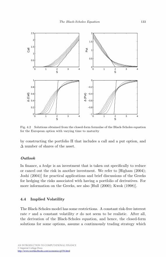
Fig. 4.1 shows the calculation of the exact formulae of the prices of a Eu-ropean call as well as a put option. It also provides the values of the deltas




corresponding to those options. In Fig. 4.2 we show the correspondingvalues versus the asset price S.

CallPut Delta.m

function [C, Cdelta, P, Pdelta] = CallPut_Delta(S,K,r,sigma,tau,div)% tau = time to expiry (T-t)

if nargin < 6div = 0.0;

endif tau > 0

d1 = (log(S/K) + (r + 0.5*sigma^2)*(tau)*ones(size(S))) / (sigma*sqrt(tau));d2 = d1 - sigma*sqrt(tau);N1 = 0.5*(1+erf(d1/sqrt(2))); N2 = 0.5*(1+erf(d2/sqrt(2)));C = exp(-div*tau) * S.*N1-K*exp(-r*(tau))*N2; Cdelta = exp(-div*tau) * N1;P = C + K*exp(-r*tau) - exp(-div*tau)*S; Pdelta = Cdelta - exp(-div*tau);

elseC = max(S-K,0); Cdelta = 0.5*(sign(S-K) + 1);P = max(K-S,0); Pdelta = Cdelta - 1;

end

Fig. 4.1 The use of closed-form solution of the Black-Scholes equation, and the deltahedging parameter

As time to maturity approaches zero, the values of the options becomecloser to the corresponding payoff functions. On the other hand, the deltasof the options have a jump at the strike price (K = 2) when the maturity(T = 5) is reached.

The following example illustrates the delta Greeks for a portfolio ofoptions. However, for simplicity, the options considered have the sameunderlying asset and the strike prices.

Example 4.1. Consider a portfolio Π consisting of a European call and aput option. Suppose the strike prices are the same: K = 2 for each. Letthe interest rate r be r = 0.03 and the volatility σ of the underlying assetbe σ = 0.25. Furthermore, assume that time to maturity is also the same:T = 5 for both options. A Matlab script is shown in Fig. 4.3, which usesthe function in Fig. 4.1.

The graphs of the values of the options and the portfolio are depictedin Fig. 4.4. First row in the figure shows the values, respectively, of theoptions and of the portfolio. The second row contains the graphs of thecorresponding deltas of the options and the portfolio.

Notice that the delta of the portfolio, ∆Π = ∆C +∆P , shown in Fig. 4.4is zero for a nonzero value of the asset price. Indeed, adding some numberof shares of the asset to the portfolio makes the portfolio riskless. Not asurprise! This number is ∆ = −(∆C +∆P ), which is obtained immediately




0 1 2 3 40

0.5

1

1.5

2

2.5

S

Cal

l

0 1 2 3 40

0.5

1

1.5

2

S

Put

0 1 2 3 40

0.2

0.4

0.6

0.8

1

S

∆ (C

all)

0 1 2 3 4−1

−0.8

−0.6

−0.4

−0.2

0

S

∆ (P

ut)

Fig. 4.2 Solutions obtained from the closed-form formulae of the Black-Scholes equationfor the European option with varying time to maturity

by constructing the portfolio Π that includes a call and a put option, and∆ number of shares of the asset.

Outlook

In finance, a hedge is an investment that is taken out specifically to reduceor cancel out the risk in another investment. We refer to [Higham (2004);Joshi (2004)] for practical applications and brief discussions of the Greeksfor hedging the risks associated with having a portfolio of derivatives. Formore information on the Greeks, see also [Hull (2000); Kwok (1998)].

4.4 Implied Volatility

The Black-Scholes model has some restrictions. A constant risk-free interestrate r and a constant volatility σ do not seem to be realistic. After all,the derivation of the Black-Scholes equation, and hence, the closed-formsolutions for some options, assume a continuously trading strategy which




sumOfCallPut Eg.m

% sumOfCallPut_Egclear all, close allS = 0:0.1:4; K = 2; r = 0.03; sigma = 0.25; T = 5;

[c, cd, p, pd] = CallPut_Delta(S, K, r, sigma, T);subplot(2,2,1), plot(S, c), hold on, plot(S, p, ’r--’)xlabel(’S’,’Fontsize’,12), ylabel(’V’,’Fontsize’,12); legend(’V_C’, ’V_P’);subplot(2,2,2), plot(S, c+p), xlabel(’S’,’Fontsize’,12)ylabel(’V_\Pi = V_C + V_P’,’Fontsize’,12)subplot(2,2,3), plot(S, cd), hold on, plot(S, pd, ’r--’)xlabel(’S’,’Fontsize’,12), ylabel(’\Delta’,’Fontsize’,12)legend(’\Delta_C’, ’\Delta_P’);subplot(2,2,4), plot(S, cd+pd), hold on, plot([0 4], [0 0], ’g-.’)xlabel(’S’,’Fontsize’,12), ylabel(’\Delta_\Pi = \Delta_C + \Delta_P’,’Fontsize’,12);print -r900 -deps ’../figures/sumOfCallPut_Eg’

Fig. 4.3 Value of a portfolio consisting of a call and a put option

0 1 2 3 40

0.5

1

1.5

2

2.5

S

V

V

C

VP

0 1 2 3 40.5

1

1.5

2

2.5

S

VΠ

= V

C +

VP

0 1 2 3 4−1

−0.5

0

0.5

1

S

∆

∆

C

∆P

0 1 2 3 4−1

−0.5

0

0.5

1

S

∆ Π =

∆C +

∆P

Fig. 4.4 Values and deltas of a portfolio consisting of a call and a put option

is not feasible in the market in order to hedge the portfolio that has beenconstructed. This is simply due to the changing number of shares ∆ = ∂V

∂S

continuously in time. Furthermore, the model does not assume the presenceof transaction costs.




In fact, you may possibly add more drawbacks to these deficiencies of theBlack-Scholes setting. Despite these restrictions and deficiencies, however,the Black-Scholes model has become so popular and was awarded with aNobel Prize! This is mainly due to the existence of a concrete, closed-form solutions to some options whose variants are traded at the market.Beyond professionals and experts in mathematical finance, a closed-formsolution means a lot for academics and, especially, for practitioners, theactual players of the market. The Black-Scholes formulae have also thebenefit of being very easy to use and understand: given the parametersthat are involved in the Black-Scholes formulae, you may directly computethe price of the options.

The only trouble seems to be the estimation of the parameters, espe-cially the estimation of the volatility σ from historical data. The estimationof µ may be easier than that of σ, even more, for pricing purposes µ dis-appears, and it is replaced by the risk-free interest rate r. It may be easierto estimate r for short term periods, and it may be a part of the optioncontract.

As it turns out, the empirical performance of the Black-Scholes formulaeis reasonably good. For options with a strike price that is not too far fromthe current price of the underlying asset price, the Black-Scholes formulaeanticipates the observed prices at the market rather well. However, foroptions that are deep out of the money , the observed prices are, in mostcases, higher than the ones suggested by the formulae. This might be partlybecause of the difficulty of estimation of the parameters r and especially σ,which are assumed to be constant in the Black-Scholes setting. It does notappear to be the case that the volatility is constant over the life time of anoption.

However, the option prices are quoted in the market so that the marketimplicitly knows or presumes the volatility. The volatility σ derived fromthese quoted prices for an option is called the implied volatility. Due to theclosed-form solutions, the Black-Scholes setting is a good candidate modelto estimate the volatility implied by the market.

If V denotes the quoted prices of an option, then the implied volatilityσ is the value of the σ for which

V = V (S, t, T, K, r, σ), (4.57)

where V = V (S, t, T, K, r, σ) denotes the model value of the option, which ismostly referred to as the theoretical price. Although the underlying model




can be any challenging one, the use of the Black-Scholes formulae is easyand illustrative. Thus, it follows from (4.57) that the implied volatility σ

is any of the zeros of the function

f(σ) = V − V (S, t, T, K, r, σ), (4.58)

which represents the difference between the observed and the theoreticalprices. In other words, the roots of the equation f(σ) = 0 are sought.Indeed, a similar root finding problem was discussed in Example 2.8 onpage 67. The premium of a pay-later contract was found to be the root ofa certain function.

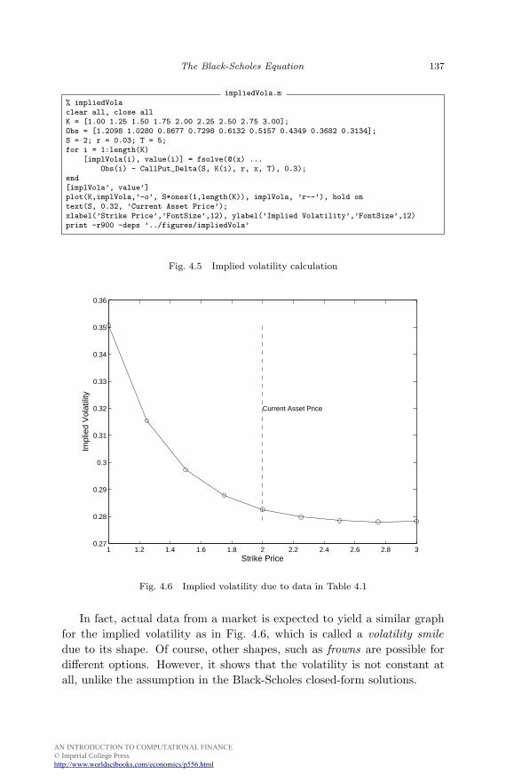
Example 4.2. This example presents the root finding problem for theimplied volatility. The data shown in Table 4.1 are totally artificial andassumed to be observed for 9 call options in the market. Each row in thetable shows the corresponding values of an option with the strike price K.

Table 4.1 Observed data

Option # Strike price K Call Option VC

1 1.00 1.20982 1.25 1.02803 1.50 0.86774 1.75 0.72985 2.00 0.61326 2.25 0.51577 2.50 0.43498 2.75 0.36829 3.00 0.3134

Assume that the current price of the underlying asset of the options isS = 2.00 and the interest rate is r = 3%. Also, suppose that the time tomaturity of all options considered is the same: T = 5. These values andthe observed data are also shown in Fig. 4.5.

The values of the implied volatility for the call options in Table 4.1 arecalculated as

σ1 = 0.3507, σ2 = 0.3153, σ3 = 0.2973, σ4 = 0.2878, σ5 = 0.2826,

σ6 = 0.2798, σ7 = 0.2784, σ8 = 0.2780, σ9 = 0.2783,

respectively. The curve corresponding to the values of the implied volatilityis depicted in Fig. 4.6.




impliedVola.m

% impliedVolaclear all, close allK = [1.00 1.25 1.50 1.75 2.00 2.25 2.50 2.75 3.00];Obs = [1.2098 1.0280 0.8677 0.7298 0.6132 0.5157 0.4349 0.3682 0.3134];S = 2; r = 0.03; T = 5;for i = 1:length(K)

[implVola(i), value(i)] = fsolve(@(x) ...Obs(i) - CallPut_Delta(S, K(i), r, x, T), 0.3);

end[implVola’, value’]plot(K,implVola,’-o’, S*ones(1,length(K)), implVola, ’r--’), hold ontext(S, 0.32, ’Current Asset Price’);xlabel(’Strike Price’,’FontSize’,12), ylabel(’Implied Volatility’,’FontSize’,12)print -r900 -deps ’../figures/impliedVola’

Fig. 4.5 Implied volatility calculation

1 1.2 1.4 1.6 1.8 2 2.2 2.4 2.6 2.8 30.27

0.28

0.29

0.3

0.31

0.32

0.33

0.34

0.35

0.36

Current Asset Price

Strike Price

Impl

ied

Vol

atili

ty

Fig. 4.6 Implied volatility due to data in Table 4.1

In fact, actual data from a market is expected to yield a similar graphfor the implied volatility as in Fig. 4.6, which is called a volatility smiledue to its shape. Of course, other shapes, such as frowns are possible fordifferent options. However, it shows that the volatility is not constant atall, unlike the assumption in the Black-Scholes closed-form solutions.




Outlook

The changes of the volatility during the life time of the options cause hedg-ing costs, hence, the volatility implied by the market has to be estimatedby the traders. There are alternative models to the Black-Scholes modelunder which options are priced and used to estimate the implied volatility.See [Joshi (2004); Hull (2000); Kwok (1998)] for those alternative models,some of which assume a stochastic volatility.

Chapter 4: The Black-Scholes Equation - Asian Scientist Magazine

Documents

Transcript of Chapter 4: The Black-Scholes Equation - Asian Scientist Magazine