CHAPTER 4 SPECIES CLASSIFICATION USING ANN METHOD...
25
69 CHAPTER 4 SPECIES CLASSIFICATION USING ANN METHOD 4.1 INTRODUCTION Biological classification is the process by which scientists group living organisms. Organisms are classified based on how similar they are. Historically, similarity was determined by examining the physical characteristics of an organism but modern classification uses a variety of techniques including genetic analysis. In molecular biology, DNA sequences are the fundamental information for each species and a comparison between DNA sequences is an interesting and basic problem. There are various open databases available in different Countries to maintain the DNA sequences of already analyzed and clarified species. When the research laboratory or organizations landed in any of an unidentified species’ DNA sequence, they need to compare that with the existing databases. From that they will find out suitable or nearer species which resembles the test data. This is called as classification or grouping. Mostly, the test DNA sequence may be a part of a gene of an organism and the available databases are very huge with billions of DNA sequence details. Also DNA sequences can be handled as bit streams. Since a DNA sequence is constructed with four bases (A, C, T, and G). There are at least 26 billion base pairs (bp) representing the various genomes available in the server of the National Center for Biotechnology Information (NCBI). Gene identification is one of the most important tasks in the study of genomes. Methods such as clustering, data mining, gene identification etc were used in DNA analysis. The objective of these methods was to facilitate collaboration between researchers and bio-informaticians by presenting cutting edge research topics and methodologies. All the above studies aim to discover genes and their characteristic expression parameters, which help to discriminate between object
Transcript of CHAPTER 4 SPECIES CLASSIFICATION USING ANN METHOD...

69
CHAPTER 4
SPECIES CLASSIFICATION USING ANN METHOD
4.1 INTRODUCTION
Biological classification is the process by which scientists group living
organisms. Organisms are classified based on how similar they are. Historically,
similarity was determined by examining the physical characteristics of an organism
but modern classification uses a variety of techniques including genetic analysis.
In molecular biology, DNA sequences are the fundamental information for
each species and a comparison between DNA sequences is an interesting and basic
problem. There are various open databases available in different Countries to
maintain the DNA sequences of already analyzed and clarified species. When the
research laboratory or organizations landed in any of an unidentified species’ DNA
sequence, they need to compare that with the existing databases. From that they will
find out suitable or nearer species which resembles the test data. This is called as
classification or grouping. Mostly, the test DNA sequence may be a part of a gene of
an organism and the available databases are very huge with billions of DNA
sequence details.
Also DNA sequences can be handled as bit streams. Since a DNA sequence
is constructed with four bases (A, C, T, and G). There are at least 26 billion base
pairs (bp) representing the various genomes available in the server of the National
Center for Biotechnology Information (NCBI).
Gene identification is one of the most important tasks in the study of
genomes. Methods such as clustering, data mining, gene identification etc were used
in DNA analysis. The objective of these methods was to facilitate collaboration
between researchers and bio-informaticians by presenting cutting edge research
topics and methodologies. All the above studies aim to discover genes and their
characteristic expression parameters, which help to discriminate between object

70
classes. So far, great effort has been put into various methods of classification of
genes for the purpose of DNA analysis.
Genomic signal processing (GSP) is a relatively new area in bio-informatics
that uses traditional digital signal processing techniques to deal with digital signal
representations and analysis of genomic data. GSP gains biological knowledge by
the analysis, processing, and use of genomic signals and translates the gained
biological knowledge into systems-based applications. Integration of signal
processing theories and methods with global understanding of functional genomics
with significant emphasis on genomic regulation is the main objective of GSP.
The whole DNA of a living organism is known as its Genome. Genomic
signals carry genomic information to all the processes that take place in an
organism. Essentially DNA is a nucleic acid that has two long strands of nucleotides
twisted in the form of a double helix and its external backbone is made up of
alternating deoxyribose sugar and phosphate molecules. The nitrogenous bases
Adenine, Guanine, Cytosine and Thymine are present in the interior portion of the
DNA in pairs. DNA and proteins can be mathematically represented as character
strings, where each character is a letter of the alphabet.
One of the vital tasks in the study of genomes is gene identification. DNA
analysis utilizes methods such as clustering, data mining, gene identification and
gene regulatory network modeling. These methods present cutting edge research
topics and methodologies for the purpose of facilitating collaboration between
researchers and bioinformaticians. Mining bioinformatics data is a rising field at the
intersection of bioinformatics and data mining. Some of them belong to the category
of data mining that decides whether or not an example not yet noticed is of a
predefined type. Increased availability of huge amount of biomedical data and the
expectant need to turn such data into useful information and knowledge is the main
reason for the recent increased attention in data mining in the biomedical industry.
Large number of research works that incorporate data mining in
bioinformatics for different purposes are available in the literature. A few important
such researches are reviewed in chapter 2. One important research of this type is the

71
identification of species or name of an organism from its gene sequence.
Characterization of the unknown environmental isolates with the genomic species is
not easy because genomic species are especially heterogeneous and poorly defined.
Identifying the species or the organism from its gene sequence is a challenging task.
In this chapter, a classification technique to effectively classify the species or name
of an organism from its DNA sequence is proposed.
In the last few decades, as the biologists have get accustomed to the use of
computers and consequently to the implementation of different complex statistical
methods, they are trying to explore multi-variate correlations between the output and
input variables more and more in detail. With the increasing accuracy and precision
of analytical measuring methods it become clear that all effects that are of interest
cannot be described by simple uni-variate and even not by the linear multivariate
correlations precise, a set of methods, that have recently found very intensive use
among biologists are the artificial neural networks. In this thesis work, a multilayer
neural network is constructed to analyze the biological data for species
identification.
Multilayer neural networks are feed forward ANN models which are also
referred to as multilayer perceptrons. The addition of a hidden layer of neurons in
the perceptron allows the solution of nonlinear problems such as the XOR, and
many practical applications (using the backpropagation algorithm). However, the
difficulty of adaptation of the weights between the hidden and input layers of the
multilayer perceptrons has dampened such architecture. With the discovery of the
back propagation algorithm by Rumelhart, Hinton & Williams in 1985, the
adaptation of the weights in the lower layers of multilayer neural networks are now
possible.
There are various kinds of string comparison tools available and they will
provide approximate matching. However most of the tools are based on exact
matching of the strings. But, the total number of sequences is rapidly increasing,
efficient methods are needed. Today’s requirement is a tool, not only for fast
matching but also for efficient sequences storage.

72
In this chapter, comparison of the existing algorithms for string matching is
analyzed for the given set of sequences. After that the same is tried with the ANN
method and the output is analyzed. Discussion on what is data mining,
Bioinformatics and neural networks are in brief. The discussion continues with the
use of neural network in datamining. In this chapter Back propagation algorithm is
also briefed.
4.2 RELATED WORKS
(Riccardo Bellazzi et al. 2007) Plenty of research works deals with the
mining knowledge from the genomic sequences. Some of the recent research works
are briefly reviewed by the authors in their paper. They have discussed that in the
past years, the gene expression data analysis that are aiming at complementing
microarray analysis with data and knowledge of various existing sources has grown
from being purely data-centric to integrative. Focusing on the evolution of gene
expression data mining techniques toward knowledge-based data analysis
approaches, they have reported on the overabundance of such techniques.
Particularly, latest developments in gene expression-based analysis methods utilized
in association and classification studies, phenotyping and reverse engineering of
gene networks have been discussed.
(Riccardo Bellazzi et al. 2007) It has been widely recognized that the genes
involved in the same biological process or with a similar function are likely to be co-
expressed. One possible way to perform gene function discovery is thus to group
genes with a similar expression pro le, consisting of gene expressions measured at
either di erent conditions or in di erent time points. The functional annotation of a
new gene can then be hypothesized on the basis of functional classes of the other,
similarly expressed genes. Because of the relative simplicity of available methods
and related visualizations that can reveal the underlying data structure, it is not
surprising that the area of DNA microarrays data analysis which has so far probably
received the greatest attention is the clustering of gene expression pro les.
Over the last couple of years and following the principal idea behind
intelligent data analysis, new e orts have been devoted to increase the performance

73
of clustering methods in terms of their robustness and stability by also considering
the available knowledge on gene function.
The gene expression data sets for ovarian, prostate, and lung cancer was
examined by (Shital Shah et al. 2007). For genetic expression data analysis, an
integrated gene-search algorithm was presented. For making predictions and for data
preprocessing (on partitioned data sets) and data mining (decision tree and support
vector machines algorithms), a genetic algorithm and correlation-based heuristics
was included in the their integrated algorithm. The knowledge, which was obtained
by the algorithm, has high classification accuracy with the capability to recognize
the most important genes. To further improve the classification accuracy, bagging
and stacking algorithms were employed. The results were compared with the literary
works. The cost and complexity of cancer detection and classification was
eventually condensed by the mapping of genotype information to the phenotype
parameters.
Locating motif in bio-sequences, which is a very significant primitive
operation in computational biology, was discussed by (Hemalatha et al. 2008).
Computer memory space requirement and computational complexity are few of the
computational requirements that are needed for a motif discovery algorithm. To
overcome the intricacy of motif discovery, an alternative solution integrating genetic
algorithm and Fuzzy Art machine learning approaches was proposed for eradicating
multiple sequence alignment process. The results that were attained by their planned
model to discover the motif in terms of speed and length were compared with the
enduring technique. By their technique, the length of 11 was found in 18 sec and
length of 15 in 24 sec, whereas the existing techniques found length of 11 in 34 sec.
When compared to other techniques, the proposed one has outperformed the
accepted existing technique. By employing MATLAB, the projected algorithm was
put into practice and with large DNA sequence data sets and synthetic data sets, it
was tested.
An interactive framework which is based on web for the analysis and
visualization of gene expressions and protein structures was described by (Ashraf S.
74
Hussein 2008). The formulation of the projected framework encountered various
confronts because of the variety of significant analysis and visualization techniques,
moreover to the survival of a diversity of biological data types, on which these
techniques function.
Data incorporated from heterogeneous resources, for instance expert-driven
data from text, public domain databases and various large scale experimental data
and the lack of standard I/O that makes it difficult to integrate the most recent
analysis and visualization are the two main challenges that directed the formulation
of the current framework. Hence, the basic novelty in their proposed framework was
the integration of the state-of -art techniques of both analysis and visualization for
gene expressions and protein structures through a unified workflow. Moreover, a
wide range of input data types are supported by it and three dimensional interactive
outputs ready for exploration by off-the-shelf monitors and immersive, 3D, stereo
display environments can be exported by it using Virtual Reality Modeling
Language (VRML).
A stomach cancer detection system, which is on the basis of Artificial Neural
Network (ANN) and the Discrete Cosine Transform (DCT), was developed by
(Ahmad M. Sarhan 2009). By employing DCT the projected system extracted the
classification features from stomach microarrays. The extracted characteristics from
DCT coefficients were applied to an ANN for further classification (tumor or non-
tumor). The microarray images that were employed were acquired from the Stanford
Medical Database (SMD). Simulation results has illustrated that a very high success
rate was produced by the proposed system.
The challenging issue in microarray technique which was to analyze and
interpret the large volume of data was discussed by (Valarmathie et al. 2009). This
can be made possible by the clustering techniques in data mining. In hierarchical and
k-means clustering techniques which are hard clustering, the data is split into
definite clusters, where each cluster has exactly one data element so that the result of
the clustering may be wrong many times.

75
The problems that are addressed in hard clustering can be resolved in fuzzy
clustering technique. Amid all fuzzy based clustering, fuzzy C-means (FCM) is best
suited for microarray gene expression data. The problem that is related with fuzzy
C-means was the amount of clusters that are to be generated for the given dataset
and that needs to be notified first. By combining the technique with a popular
probability related Expectation Maximization (EM) algorithm, it can be solved to
model the cluster structure of gene expression data and it has offered the statistical
frame work. Determining the accurate number of clusters and its efficient
interpretation is the main purpose of the projected hybrid fuzzy C-means technique.
Explorative studies in support of solutions to facilitate the analysis and
interpretation of mining results was described by (Belmamoune et al. 2010). A
solution that was located in the extension of the Gene Expression Management
System (GEMS) was described, i.e. an integrative framework for spatio-temporal
organization of gene expression patterns of zebra fish to a framework that supports
data mining, data analysis and patterns interpretation.
As a proof of principle, the GEMS is provided with data mining functionality
which is appropriate to monitor spatio-temporal, thus generating added value to the
submission of data for data mining and analysis. On the basis of the availability of
domain ontologies, the analysis of the genetic networks was done which vigorously
offers the meaning to the discovered patterns of gene expression data. Grouping of
data mining with the already accessible potential of GEMS considerably augments
the existing data processing and functional analysis strategies.
4.3 BASIC BUILDING BLOCKS
This section introduces the concept of bioinformatics and the applications of
data mining, and neural networks in biological databases with simple block diagram.
4.3.1 Data Mining
Data mining is the process of discovering interesting patterns from massive
amounts of data. In biological databases, the amount of data available is in trillions
76
of bps. In Data mining, as a process of knowledge discovery, the steps typically
involves - data cleaning, data integration, data selection, data transformation, pattern
discovery, pattern evaluation, and knowledge presentation.
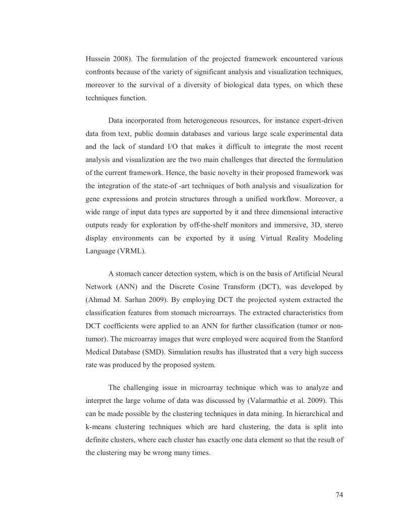
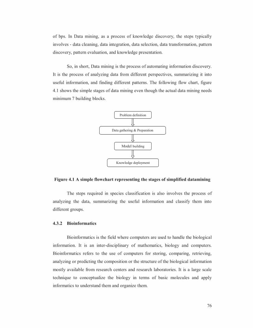
So, in short, Data mining is the process of automating information discovery.
It is the process of analyzing data from different perspectives, summarizing it into
useful information, and finding different patterns. The following flow chart, figure
4.1 shows the simple stages of data mining even though the actual data mining needs
minimum 7 building blocks.
Figure 4.1 A simple flowchart representing the stages of simplified datamining
The steps required in species classification is also involves the process of
analyzing the data, summarizing the useful information and classify them into
different groups.
4.3.2 Bioinformatics
Bioinformatics is the field where computers are used to handle the biological
information. It is an inter-disciplinary of mathematics, biology and computers.
Bioinformatics refers to the use of computers for storing, comparing, retrieving,
analyzing or predicting the composition or the structure of the biological information
mostly available from research centers and research laboratories. It is a large scale
technique to conceptualize the biology in terms of basic molecules and apply
informatics to understand them and organize them.
Problem definition
Data gathering & Preparation
Model building
Knowledge deployment

77
Figure 4.2 The block diagram of Bioinformatics
The biological database is broadly classified as structural biological
database, sequential biological database and others. Here the concentration is on
sequential biological database as the DNA sequence is falling under this category.
The following figure shows the categories falling under biological database.
Biological databases
Structure Sequence Others
Protein Nucleic acid
Figure 4.3 Broad classification of Biological Database
4.3.3 Neural Network
A machine that is designed to imitate the way human brain performs a
particular task or function is called as neural network. To implement neural network
in digital computer, either electronic components or software simulators will be
used. To make neural network to perform useful computations, the process of
New Knowledge
Computational
Biology
Bioinformatics
Computational
model
Biological data

78
learning is used. Based on the massive interconnections, the performance of a neural
network will vary. The computing cells of neural networks were referred as neurons
or processing units
Figure 4.4 A typical neural network
The big Strengths of Neural Networks are, it is generalized and self
organized. The neural network will work with inadequate and volatile knowledge
base also. People can use incorrect or incomplete or noisy inputs to recall the
information. This characteristic of the neural network is best suited for biological
databases as most of them or noisy and incomplete. Even though the training phase
takes reasonable time, the project development phase will take short time only. Even
biologists prefer this characteristic is best suited for biological database.
4.3.4 Neural Networks and Data Mining
From the above discussions, one can find the clarity about the relationships
of biological data, bioinformatics, data mining and the neural networks. So to
consolidate it, the following steps are needed.
Develop a Neural Network Applications for the classification problem.
Check that the neural network approach is appropriate and select an appropriate
paradigm. Once that is done, start to give inputs by selecting proper inputs and facts.
Once the inputs are in their proper format, start to train the network. Once the
Input
Input
Input
Input Input layer
Hidden
layer
Output
layer

79
network is trained, test it with known data and check its perfectness. Now the neural
network application is ready for run. Run the neural network for different unknown
data sets and find out the similarities of the existing data and the test data. Table it.
Run the same set of data for different string comparison algorithms and compare it
with neural network’s output. From the table one can conclude which is the best
algorithm for the species classification.
4.3.5 Example for Neural Network Tool
There are some standard neural network applications available in the market.
For example, according to the website for NeuralWare (2005):
“NeuralWorks Predict® is an integrated, state-of-the-art tool for rapidly
creating and deploying prediction and classification applications. Predict® combines
neural network technology with genetic algorithms, statistics, and fuzzy logic to
automatically find optimal or near-optimal solutions for a wide range of problems.”
The University of California at Irvine Machine Learning Repository had
used the NeuralWorks Predict® software on data sets for variety of applications.
The applications vary from USA Space Shuttle database to wine recognition
databases. One can find out from this discussion that NeuralWorks Predict® can
work with any sort of big databases. So biologists can even use this product for
biological databases analysis too.
4.4 PATTERN MINING FROM DNA SEQUENCE
The first and initial stage of the proposed technique mines the nucleotide
pattern from the DNA sequence. At this stage, patterns formed by different
combinations of nucleotides are mined using a novel mining algorithm. Let g be the
DNA sequence, which is a combination of four nucleotides A, G, C and T. For
instance, a sample DNA sequence is given as CGTCGTGGAA. From the sequence,
the mining algorithm extracts different nucleotide patterns and their support. The
algorithm is comprised of two stages, namely, pattern generation and support
finding. In pattern generation, patterns with different length are generated whereas in

80
support finding, support values for every generated pattern are determined from the
DNA sequence. The basic structure of the algorithm is given as a block diagram in
Figure 5.
Figure 4.5 Block diagram of the pattern mining algorithm
4.4.1 Pattern generation
In pattern generation, different possible combinations of nucleotide base
pairs are generated. As a reference, a base set B is generated with cardinality
4|| B , which has the elements },,,{ TCGA . Let, max,,2,1};{ LlPl , be the pattern
set to be generated, where, maxL is the maximum length of a pattern in a pattern set.
The pattern set is generated as follows
)()()( 211)()( lklkl aBaBaBPP ll (1)
where,ll Bk ||,,2,1)(, ||,,,1 21 Baaa l and )()()( 21 laBaBaB is a set of
different combinations of nucleotide bases. Eq. (1) operates with the criterions,
)()( 1 ll klkl PP and ll PaBaBaB )()()( 21 . Eq. (1) formulated for pattern
generation is analyzed using an example.
Example 1: To generate a single length pattern set 1P , i.e. 1l . As per the Eq. (1), a
single indexing variable 1a is generated. At every k i.e. 41 tok and for its
corresponding 1a , the obtained )( 1aB and 1)1(1 K
P are tabulated in Table I.
Extract
nucleotide
patterns
Generate
pattern set
Determine
pattern
support
Generate
constructive
dataset
DNA
sequence
Mined
knowledge

81
Table 4.1 Different combinations and pattern sets generated for
every 1a and k
k a1 B(a1) 11 )1(kP
1 1 A {}
2 2 G {A}
3 3 C {A,G}
4 4 T {A,G,C}}
The 1P obtained from every thk iteration is integrated and hence 1P is
obtained as },,,{}{ 1 TCGAP .
4.4.2 Determination of pattern support
The support, which has to be determined for every extracted pattern,
describes the DNA attribute. By performing a window based operation over the
sequence g , the support can be determined. Window of sequences are determined
for different lengths as follows
)1,,1,()( ljjjgjwl (2)
Once the window of sequences is extracted support is determined for the
mined patterns. The pseudo code, which is given below, describes the procedure to
determine the support for every pattern.
Figure 4.6 Pseudo code to determine support for every mined pattern
Initialize C to zero
read window of sequence w
for every l - length pattern, lP
for each element i in )(, iPP ll
for each window of sequence )( jwl
if )(iPl and )( jwl are same
increment )(iCl
end if
end for
end for
end for
Return C

82
The obtained C for each different length pattern has the support for all the
elements that are present in the corresponding pattern set. From the mined pattern
and its corresponding support, a constructive dataset is generated.
4.4.3 Constructive dataset generation
A raw dataset is generated using the aforesaid mining algorithm. But the
dataset is not constructive for further operation. In this stage, a constructive dataset
is generated from the mined dataset, which comprises of patterns with different
lengths and their support. To accomplish this, firstly the patterns which have length
2l are taken. From the pattern set, the modified and constructive dataset is
generated as given in Figure 4.7.
A G C T
A C2(1) C2(2) C2(3) C2(4)
G C2(5) C2(6) C2(7) C2(8)
C C2(9) C2(10) C2(11) C2(12)
T C2(13) C2(14) C2(15) C2(16)
AA C3(1) C3(2) C3(3) C3(4)
AG C3(5) C3(6) C3(7) C3(8)
AC C3(9) C3(10) C3(11) C3(12)
AT C3(13)
Figure 4.7 A general structure of the proposed constructive dataset
In the constructive dataset, all the patterns except single length pattern are
considered. Hence, the dataset is of size 441maxL
. The generated constructive
dataset belongs to a particular gene sequence. Similarly, the constructive dataset for
different sequences are generated. Hence, the final dataset )( z
xyG ;1max4,,2,1
Lx ,

83
43,2,1 andy and gNz ,,2,1 is obtained, which is subjected to further
processing.
4.5 MPCA-BASED DIMENSIONALITY REDUCTION
In all tensor modes, the multilinear algorithm MPCA captures most of the
variation present in the original tensors by seeking those bases in each mode that
allow projected tensors and performs dimensionality reduction. Initially, in the
process of dimensionality reduction, the distance matrix for every thz matrix is
determined as follows,
)()( zz GD (3)
where,
1
0
)(1 GN
z
z
xy
G
xy GN
(4)
Using Equation (3) and by determining the mean matrix for )( zG using Eq.
(4), the distance matrix can be calculated. Then with mode 2, tensor representations
)(
1
zT and )(
2
zT are given to the obtained distance matrix. A projection matrix is
determined as follows,
1
0
)()(GN
z
Tzz TT (5)
For both )(
1
zT and)(
2
zT , the projection matrix ( 1 and 2 ) are determined
using the generalized form of calculation given in Equation (5). For 1 and 2 , the
corresponding eigenvectors 1E and 2E and the corresponding eigenvalues 1 and 2
are determined by subjecting the projection matrix to a generalized eigenvector
problem. The rows of the eigenvector are arranged based on the index of the
eigenvalues sorted in the descending order. The modified eigenvector '
1E and
'
2E are
obtained by transposing the arranged eigenvector. The cumulatively distributed

84
eigenvalues for the sorted eigenvalues are generally determined using the following
equation.
1||
0
'
x
sort
x
cdf
xx (6)
The sorted eigenvalues sort
x and the cumulatively distributed eigenvalues
cdf
x of Equation (6), can be determined as
cdfx
sortx
cdfx 1 (7)
where,sortcdf
00 at 0x . The new dimension T is calculated from the obtained
'
x , using a dimensional threshold TD . To accomplish this, the indices of all
eigenvalues that satisfy the condition Tx D' are identified. Then, by extracting the
first T rows of '
1E and
'
2E , the corresponding dimensionality reduced eigenvectors
''
1E and
''
2E are determined. For the ''
1E and
''
2E , again tensor matrices but )(
1
zT and
)(
2
zT times are determined. The process followed for projection matrix is repeated for
the tensor matrices to obtain new
x1 and
new
x2 and
newE1 and newE2 . The weight of both
the tensor eigenvalues are determined asnew
x
new
x
w
x 21. Then, the dimensionality
reduced matrix )( z
G of size TR NN , is obtained by using the MPCA projections,
where, RN can be determined as21
. TTRN .
4.6 CLASSIFICATION USING ANN
For GN gene sequences, the dimensionality reduced gene patterns and their
support are provided by the MPCA. Using ANN, the class of the original sequence
can be identified using the dataset. Two classical operations, training and testing are
involved in the classification. The neural network is trained using the GN pattern
dataset. Here, the process is performed using multilayer feed forward neural

85
network, depicted in Figure 4.8. RN input nodes, HN hidden nodes and an output
node are present in the network.
Figure 4.8 The multilayer feed forward neural network used
in the proposed technique
Before performing any task, the ANN must be trained. Once trained, the
ANN capably identifies the species by finding the class of the gene sequence. The
training phase and classification phase of the ANN are described below.
4.6.1 Training Phase
Back Propagation (BP) algorithm is used to train the constructed feed
forward network. The step-by-step procedure utilized in the training process is given
below.
1. Assign arbitrary weights generated within the 1,0 interval to links between
the input layer and hidden layer as well as hidden layer and output layer.
2. Using Equations (8), (9) and (10), determine the output of input layer, hidden
layer and output layer respectively by inputting constructive dataset to the
network.
W11
2WRN
1WRN
HN2W
W12
W21
HN1W
NR
1
2
NH
1
2
G(z)(NR)
W11
W22
HRNNW
G(z)(1)
G(z)(2)
W21
1NHW
S
1

86
RN
rrqq rGWh
1
)1()( ; RNr ,,2,1 , HNq ,,2,1 (8)
)1(
)1(
2
)2(
1
1h
h
e
eh (9)
)2(hS (10)
where, Equation (8) is the basis function for the input layer and Equation (9)
and (10) are the activation functions for hidden and output layer, respectively.
3. Determine BP error using
1
0
1 GN
ppT
G
SSN
e (11)
where, e is the BP error,
TS is the target output
4. By adjusting the weights of all the neurons based on the determined BP
error, obtain new weights using
WWW oldnew(12)
In Equation (12), the weight to be changed W depends on the rate of
network learning and the obtained network output pS for the thp gene sequence
and it is determined using the formula eSW p .. .
5. Until the BP error gets minimized to a minimum extent, repeat the process
from step 2. The termination criterion for practical cases, is 1.0e .

87
4.6.2 Classification Phase
In the classification phase, the network finds the class of a given or test gene
sequence and determines the species to which it belongs. The same processes
performed on the training sequence are repeated for the test sequence testg . Using the
mined patterns and their support, the constructive nucleotide dataset is generated.
Subsequent to dimensionality reduction of the generated dataset they are tested in a
neural network. The neural network decides the class of the species to which the
gene sequence belongs.
4.7 IMPLEMENTATION RESULTS
The proposed technique is implemented in the working platform of
MATLAB (version 7.10) and the technique is evaluated using the DNA sequence of
two different organisms, Brucella Suis and Caenorhabditis elegans (C. elegans). The
evaluation process is performed using 10-fold cross validation test. Here, nucleotide
patterns are mined with 5maxL . The nucleotide patterns for 3and2l and their
corresponding support are given in Table 4.2. In Fig. 4.5, different length patterns
and their support are depicted and the constructive dataset that is generated from the
pattern set is given in Table 4.3.
Table 4.2: Mined nucleotide patterns from the DNA sequence of
Brucella Suis and C.elegans
(a) 2l
Species
S.
NoPattern
Support
Brucella suis C-elegans
1 aa 169042 168149
2 ag 56284 59645
3 ac 53509 54824
4 at 100894 101778
5 ga 72354 72651
6 gg 45341 45368
7 gc 46001 43023
8 gt 53423 56002
9 ca 67662 69882
10 cg 47630 40344

88
Species
S.
NoPattern
Support
Brucella suis C-elegans
11 cc 47205 44205
12 ct 57377 58316
13 ta 70670 73713
14 tg 67864 71687
15 tc 73159 70695
16 tt 171584 169717
(b) 3l (a part of the pattern is given)
Species
S.
NoPattern
Support
Brucella suis C-elegans
1 aaa 86090 83349
2 aag 17627 18623
3 aac 18374 19422
4 aat 46951 46755
5 aga 19089 19871
6 agg 11100 10442
7 agc 11318 12264
8 agt 14777 17068
9 aca 17239 17901
10 acg 10577 9453
11 acc 10491 10676
12 act 15202 16794
13 ata 20142 21368
14 atg 15783 16752
15 atc 17406 16451
16 att 47563 47207
Figure 4.9 Support obtained for different length patterns
1199994
1199995
1199996
1199997
1199998
1199999
1200000
2 3 4 5
Pattern Length
Su
pp
ort
Brucella suis
C-elegans

89
Table 4.3 Constructive dataset generated from the mined
nucleotide patterns (a) and (b)
Table 4.3(a) pattern 2l
Species
S.NoBrucella suis c-elegans
A G C T A G C T
1 A 169042 56284 53509 100894 168149 59645 54824 101778
2 G 72354 45341 46001 53423 72651 45368 43023 56002
3 C 67662 47630 47205 57377 69882 40344 44205 58316
4 T 70670 67864 73159 171584 73713 71687 70695 169717
Table 4.3 (b) Pattern 3l (a part of the pattern is given).
Species
S.
No
Brucella suis c-elegans
A G C T A G C T
1 AA 86090 17627 18374 46951 83349 18623 19422 46755
2 AG 19089 11100 11318 14777 19871 10442 12264 17068
3 AC 17239 10577 10491 15202 17901 9453 10676 16794
4 AT 20142 15783 17406 47563 21368 16752 16451 47207
5 GA 31140 13379 10257 17578 31355 13670 10422 17204
6 GG 14729 8619 11555 10438 14982 9275 9700 11411
7 GC 13025 9601 12066 11309 13656 7494 9646 12227
8 GT 12136 12780 10458 18049 12976 12650 10000 20376
9 CA 26644 12400 12801 15817 27422 13532 12501 16427
10 CG 16283 10873 9652 10822 13747 9848 7594 9155
11 CC 15108 11450 9503 11144 15133 9631 9315 10126
12 CT 13210 12537 13724 17906 12775 13648 13226 18667
13 TA 25167 12878 12077 20548 26023 13819 12479 21392
14 TG 22253 14749 13476 17386 24051 15803 13465 18368
15 TC 22290 16002 15145 19722 23192 13766 14568 19169
16 TT 25182 26764 31571 88066 26594 28637 31018 83467
The pattern data and constructive dataset given in Tables 4.2 and 4.3 are
generated from one of the ten folds of gene sequence of Brucella suis. Thus, from all

90
the ten folds of gene sequence of both Brucella suis and C. elegans, the pattern data
have been mined and constructive datasets have been generated. The generated ten
folds of data are used to train the neural network. The results obtained from network
training are given in Figure 4.10.
Fig. 4.10(a)
Fig. 4.10(b)

91
Fig. 4.10(c)
Figure 4.10: Performance of training and test results from ANN: (a)
Network performance, (b) Training evaluation and (c) Regression analysis.
Once the training process has been completed, the technique is validated
using the test sequence. The results obtained from 10-fold cross validation are given
in Table 4.4.
Table 4.4 Performance evaluation using 10-fold cross validation results
Rounds in cross
validation
Species
Brucella suis c-elegans
ANN
Output
Classification
Result
ANN
Output
Classification
Result
1 0.2421 TP 0. 5171 TP
2 0.0769 TP 0. 6272 TP
3 0.0828 TP 0. 6361 TP
4 0.2634 TP 0. 8974 TP
5 0.2493 TP 0. 6063 TP
6 0.2613 TP 0. 0141 TN

92
Rounds in cross
validation
Species
Brucella suis c-elegans
ANN
Output
Classification
Result
ANN
Output
Classification
Result
7 0.5277 TN 0. 9163 TP
8 0.3616 TP 0. 6714 TP
9 0.5849 TN 0. 5103 TP
10 0.2143 TP 0. 5142 TP
Mean Classification
Accuracy 80% 90%
From the results, it can be seen that when a gene sequence is given to the
proposed technique it identifies the corresponding species. Here, the technique is
evaluated with the DNA sequence of only two genes. The technique is developed in
such a way that it can be applied to any kind of DNA sequence. The test results
claim that the performance of the technique reaches a satisfactory level.
4.8 DISCUSSION
In this chapter, a species identification technique by integrating data mining
technique with artificial intelligence is proposed. Initially, the nucleotide patterns
have been mined effectively. The resultant has been subjected to MPCA-based
dimensionality reduction and eventually classified using a well-trained neural
network. The implementation results have shown that the proposed technique
effectively identifies the organism from its gene sequence and so the species.
Moreover, results obtained from 10-fold cross validation have proved that the
organism can be identified even from a part of the DNA sequence. Though the
technique has been tested with the DNA sequence of only two organisms, the 10-
fold cross validation results have reached a remarkable performance level. From the
results, it can be hypothetically analyzed that a technique, which identifies the
organism only with a part of gene sequence, have the ability to classify any kind of
organism and so the species.

93
4.9 CONTRIBUTION
The outcome of this work is published as a paper in the international journal
titled “IJACSA - International Journal of Advanced Computer Science and
Applications”, Volume 3, No.8, 2012, pp. 104 – 114, titled “An Effective
Identification of Species from DNA Sequence: A Classification Technique by
Integrating DM and ANN”.