Chapter 4

River flow

Much of the environment consists of fluids, and much of this book is therefore con-cerned with fluid mechanics. Oceans and atmosphere consist of fluids in large scalemotion, and even later, when we deal with more esoteric subjects: the flow of glaciers,convection in the Earth’s mantle, it is within the context of fluid mechanics that weformulate relevant models. This chapter concerns one of the most obvious commonexamples of a fluid in motion, that of the mechanics of rivers.

Fluid mechanics in the environment is, however, altogether different to the subjectwe study in an undergraduate course on viscous flow, and the principal reason for thisis that for most of the common environmental fluid flows with which we are familiar,the flow is turbulent. (Where it is not, for example in glacier flow, other physicalcomplications obtrude.) As a consequence, the models which we use to describe theflow are different to (and in fact, simpler than) the Navier-Stokes equations.

4.1 The hydrological cycle

Rainwater which falls in a catchment area of a particular river basin makes its wayback to the ocean (or sometimes to an inland lake) by seepage into the ground,and then through groundwater flow to outlet streams and rivers. In severe stormconditions, or where the soil is relatively impermeable, the rainfall intensity mayexceed the soil infiltration capacity, and then direct runoff to discharge streams canoccur as overland flow. Depending on local topography, soil cover, vegetation, oneor other transport process may be the norm. Overland flow can also occur if the soilbecomes saturated. The hydrological cycle is completed when the water, now backin the ocean, is evaporated by solar radiation, forming atmospheric clouds which arethe instrument of precipitation.

River flow itself occurs on river beds that are typically quasi-one-dimensional,sinuous channels with variable and rough cross-section. Moreover, if the channeldischarge is Q (m3 s−1), and the wetted perimeter length of the cross section is l (m),then an appropriate Reynolds number for the flow is

Re =Q

νl, (4.1)

223

where ν = µ/ρ is the kinematic viscosity (and µ is the dynamic viscosity). If l = 20m, ν = 10−6 m2 s−1, Q = 10 m3 s−1, then Re ∼ 0.5 × 106. Inevitably, river flowis turbulent for all but the smallest rivulets. A different measure of the Reynoldsnumber is

Re =uh

ν, (4.2)

where u is mean velocity and h is mean depth. In a wide channel, we have that thewidth is approximately l, so that Q ≈ ulh, and this gives the same definition as (4.1).Thus, to model river flow, and to explain the response of river discharge to stormconditions, as measured on flood hydrographs, for instance, one must model a flowwhich is essentially turbulent, and which exists in a rough, irregular channel.

The classical way in which this is done is by applying a time average to theNavier-Stokes equations, which leads to Reynolds’ equation, which is essentially likethe Navier-Stokes equation, but with the stress tensor being augmented by a Reynoldsstress tensor. The procedure is described in appendix B .

For a flow u = (u, v, w) which is locally unidirectional on average, such as that ina river, we may take the mean velocity u = (u, 0, 0), and then the x component ofthe momentum equation becomes

ρ∂

∂z(u′w′) ≈ −∂p

∂x+ µ

∂2u

∂z2, (4.3)

because in a shallow flow, the other Reynolds stress terms are smaller. Integrationover the depth shows that the resistance to motion is provided by the wall stress τ ,and this is

τ = µ∂u

∂z+ {−ρu′w′}, (4.4)

evaluated at the wetted perimeter of the flow. Strictly, the Reynolds stress vanishesat the boundary (because the fluid velocity is zero there), and the molecular stresschanges rapidly to compensate, in a very thin laminar wall layer. Normally oneevaluates (4.4) just outside this layer, close to but not at the boundary, where themolecular stress is negligible and the Reynolds stress is parameterised in some way.A common choice is to use a friction factor, thus

τ = fρu2, (4.5)

where the dimensionless number f (called the friction factor) is found to dependrather weakly on the Reynolds number.1 A crude but effective assumption is simplythat f is constant, with a typical value for f of 0.01.

4.2 Chezy’s and Manning’s laws

Our starting point is that the flow is essentially one-dimensional: or at least, we focuson this aspect of it. As well as the cross sectional area (of the flow) A and discharge

1More precisely, the stress should be τ = fρ|u|u, since the friction acts in the opposite directionto the flow. For unidirectional flows, this reduces to (4.5). Later (in section 4.5.3), we will have needfor this more precise formula.

224

Q, we introduce a longitudinal, curvilinear distance coordinate s, and we assume thatthe river axis changes direction slowly with s. Then conservation of mass is, in itssimplest form,

∂A

∂t+

∂Q

∂s= M. (4.6)

This source term M represents the supply to the river due to infiltration seepage andoverland flow from the catchment.

(4.6) must be supplemented by an equation for Q as a function of A, and thisarises through consideration of momentum conservation. There are three levels atwhich one may do this: by exact specification, as in the Navier-Stokes momentumequation; by ignoring inertia and averaging, as in Darcy’s law; and most simply, byignoring inertia and applying a force balance using a semi-empirical friction factor.We begin by opting for this last choice, which should apply for sufficiently ‘slow’ (insome sense) flow. Later we will consider more complicated models.

We have already defined the Reynolds number Re in terms of Q and A, or equiv-alently a mean velocity u = Q/A and a channel depth d ∼ A1/2. ‘Slow’ here means asmall Froude number, defined by

Fr =u

(gd)1/2=

Q

g1/2A5/4. (4.7)

If Fr < 1, the flow is tranquil; if Fr > 1, it is rapid. Gravity is of relevance, since theflow is ultimately due to gravity.

Now let l be the wetted perimeter of a cross section, and let τ be the mean shearstress exerted at the bed (longitudinally) by the flow. If the downstream angle ofslope is α, then a force balance gives

lτ = ρgA sin α, (4.8)

where ρ is density. For turbulent flow, the shear stress is given by the friction law

τ = fρu2, (4.9)

where the friction factor f may depend on the Reynolds number. Since

u = Q/A, (4.10)

and defining the hydraulic radius

R = A/l, (4.11)

we derive the relationsu = (g/f)1/2R1/2S1/2, (4.12)

whereS = sin α, (4.13)

and

Q =

(g

fl

)1/2

A3/2S1/2. (4.14)

225

For wide, shallow rivers, l is essentially the width. For a more circular cross-section,then l ∼ A1/2, and

Q = (g/f)1/2A5/4S1/2. (4.15)

The relation (4.12) is the Chezy velocity formula, and C = (g/f)1/2 is the Chezyroughness coefficient. Notice that the Froude number, in terms of the hydraulicradius, is

Fr =u

(gR)1/2= (S/f)1/2, (4.16)

and tranquillity (at least in uniform flow) is basically due to slope.Alternative friction correlations exist. That due to Manning is an empirical for-

mula to fit measured stream velocities, and is of the form

u = R2/3S1/2/n′ (4.17)

where Manning’s roughness coefficient n′ takes typical values in the range 0.01–0.1m−1/3 s, depending on stream depth, roughness, etc. Manning’s law can be derivedfrom an expression for the shear stress of the form (cf. (4.9))

τ =ρgn′2u2

R1/3. (4.18)

For Manning’s formula, we have

Q ∼ A4/3 if R ∼ A1/2,

Q ∼ A5/3 if l is width, R = A/l ∼ A. (4.19)

Thus we see that for a variety of stream types and velocity laws, we can pose arelation between discharge and area of the form

Q ∼ Am+1, m > 0, (4.20)

with typical values m = 14 – 2

3 . In practice, for a given stream, one could attempt tofit a law of the form (4.20) by direct measurement.

4.3 The flood hydrograph

Suppose in general that

Q =cAm+1

m + 1. (4.21)

We can nondimensionalise the equation for A so that it becomes

∂A

∂t+ Am ∂A

∂s= M, (4.22)

a first order nonlinear hyperbolic equation, also known as a kinematic wave equation,whose solution can be written down. The source term M is in general a function of

226

0

1

2

-3 -2 -1 0 1 2 3 4

A

s

Figure 4.1: Formation of a shock wave in the solution of (4.22) (cf. figure 1.14).

s and t, but for simplicity we take it to be constant here. Suppose the initial data isparameterised as

A = A0(σ), s = σ > 0, t = 0. (4.23)

Then the characteristic equations are

dA

dt= M,

ds

dt= Am, (4.24)

whence

A = A0(σ) + Mt, s = σ +(A0 + Mt)m+1 − Am+1

0

M(m + 1), (4.25)

thus

A = Mt + A0

[s−

{Am+1 − (A−Mt)m+1

M(m + 1)

}](4.26)

determines A implicitly.We can see from (4.26) that this solution applies for sufficiently small t or large s,

since we must have σ > 0. For larger t, the characteristics are those emanating froms = 0, where the boundary data is parameterised by

A = 0, s = 0, t = τ, (4.27)

and the solution is the steady state

Am+1

m + 1= Ms. (4.28)

227

This steady state is applicable above the dividing characteristic in the (s, t) planeemanating from the origin, which is

s =Mmtm+1

m + 1. (4.29)

Thus any initial disturbance to the steady state is washed out of the system in a finitetime (for any finite s).

From (4.26) we can calculate∂A

∂sexplicitly in terms of t and the characteristic

parameter σ, and the result is

∂A

∂s=

A′0

1 +A′

0

M{(A0 + Mt)m − Am

0 }. (4.30)

It is a familiar fact that humped initial conditions A0(σ) will lead to propagation ofa kinematic wave, and then to shock formation, as shown in figure 4.1, when ∂A/∂sreaches infinity. From (4.30), we see that this occurs on the characteristic throughs = σ for t > 0 if A′

0 < 0, when

t = tσ =1

M

[(−M

A′0

+ Am0

)1/m

− A0

], (4.31)

and a shock forms when t = minσ

tσ > 0. Thereafter a shock exists at a point sd(t),

and propagates at a rate given, by consideration of the integral conservation law

∂

∂t

∫ s2

s1

A ds = −[Q]s2s1

, (4.32)

by

sd =[Q]sd+

sd−

[A]sd+sd−

. (4.33)

As an application, we consider the flood hydrograph, which measures dischargeat a fixed value of s as a function of time. Suppose for simplicity that M = 0 (thecase M > 0 is considered in question 4.7). As an idealisation of a flood, we consideran initial condition

A ≈ A∗δ(s) at t = 0, (4.34)

where δ(s) is the delta function, representing the input to the river by overland flowafter a short period of localised rainfall. Either directly, or by letting M → 0 in(4.26), we have A = A0(s − Amt), and it follows that A ≈ 0 except where s = Amt.The humped initial condition causes a shock to form at sd(t), with sd(0) = 0, and wehave

A = 0, s > sd,

A = (s/t)1/m, s < sd, (4.35)

228

sd

A

s

Figure 4.2: Propagation of a shock front.

as shown in figure 4.2.The shock speed is given by

sd = (Q/A)|sd− =Am

m + 1

∣∣∣∣sd−

=sd

(m + 1)t, (4.36)

whence sd ∝ t1/(m+1). To calculate the coefficient of proportionality, we use conser-vation of mass in the form ∫ sd

0

A ds = A∗, (4.37)

whence, in fact,

sd =

[(m + 1)A∗

m

]m/(m+1)

t1/(m+1). (4.38)

Denoting b = [(m + 1)A∗/m]m/(m+1), the flood hydrograph at a fixed station s = s∗

is then as follows. For t < t∗, where

t∗ = (s∗/b)m+1, (4.39)

Q = 0. For t > t∗, A = (s∗/t)1/m, and thus

Q =s∗(m+1)/m

(m + 1)t−(m+1)/m. (4.40)

This result is illustrated in figure 4.3, together with a typical observed hydrograph.The smoothed observation can be explained by the fact that a more realistic initialcondition would have delivery of the storm flow over an interval of space and time.More importantly, one can expect that a more realistic model will allow diffusiveeffects.

229

Q

s

Figure 4.3: Ideal (full line) and observed (dotted line) hydrographs.

4.4 St. Venant equations

We now re-examine the momentum equation, which we previously assumed to bedescribed by a force balance. Again consider the equations in dimensional form. Forthe remainder of the chapter we take M = 0, largely for simplicity. Conservation ofmass can then be written in the form

∂A

∂t+

∂

∂s(Au) = 0, (4.41)

where the mean velocity u is defined by

u =Q

A, (4.42)

and then conservation of momentum (from first principles) leads to the equation(adopting the friction law (4.9))

ρ∂(Au)

∂t+ ρ

∂

∂s(Au2) = ρgAS − ρlfu2 − ∂

∂s(Ap), (4.43)

where p is the mean pressure. Now the pressure is approximately hydrostatic, thus

p ≈ ρgz where z is depth. Then pA ≈∫

12ρgh2dx where h is total depth and x is

width, and thus∂

∂s(Ap) = ρg

∫

A

∂h

∂sdA; (4.44)

230

if we suppose ∂h/∂s is independent of x, we find2

∂

∂s(Ap) = ρgA

∂h

∂s, (4.45)

where h is the mean depth. Using (4.41), (4.43) reduces to

ut + uus = gS − flu2

A− g

∂h

∂s. (4.46)

Equations (4.41) and (4.46) are known as the St. Venant equations.3

4.4.1 Non-dimensionalisation

We choose scales for u = Q/A, t, s, A, R (the hydraulic radius, = A/l), h as follows,in keeping with the assumed balances adopted earlier:

Au ∼ Q, gS ∼ lfu2

A=

fu2

R,

t ∼ s

u, s ∼ d

S, h, R ∼ d, (4.47)

where we can suppose Q is a typical observed discharge, and d is a typical observeddepth. Explicitly, the scales are

[h], [R] = d, [s] =

d

S,

[u] =

(gdS

f

)1/2

, [t] =

(fd

gS3

)1/2

, [A] = Q

(f

gdS

)1/2

, (4.48)

and we put u = [u]u∗, etc., and drop asterisks. The resulting equations are

At + (Au)s = 0,

F 2[ut + uus] = 1− u2

R− hs, (4.49)

2The assumption that ∂h/∂s is constant across the stream means that along a transverse sectionof the river, the surface is horizontal. This is really due to the smallness of the width comparedto the length. It is importantly not exactly true for meandering rivers, but is still a very goodapproximation.

3Note that the derivation of (4.46) assumes a constant slope S. If the slope is varying, thenthe derivation is still valid providing S is the local bed slope. If we then take S to be the averagedownstream slope, and denote the bed by z = b(s) and the surface by z = η(s), we have the localslope S = S − bs, and thus S − hs = S − ηs, and thus (4.46) still applies for varying bed slope whenS denotes the (constant) mean slope, providing we replace h by η. All of this supposes that b doesnot vary with x, i. e., the channel section is rectangular.

231

where we would choose h ∼ R ∼ A for a wide channel, h ∼ R ∼ A1/2 for a roundedchannel. In particular, for a wide channel, we have R = h, so that the momentumequation can be written

(wh)t + (wuh)s = 0,

F 2(ut + uus) = 1− u2

h− hs, (4.50)

since A = wh, where w is the (dimensionless) width. As before, the Froude numberF is given by

F =[u]

(gd)1/2=

(S

f

)1/2

. (4.51)

4.4.2 Long wave and short wave approximation

To estimate some of these scales, we take d = 2 m, u = 1 m s−1 and S = sin α = 0.001,

typical lowland valley values. We then have the length scale [s] =d

S∼ 2 km, and

the time scale t ∼ 33 minutes, and in some sense these are the natural length andtime scales for the dynamic river response. However, it is fairly clear that these scalesare not appropriate either for variations over the length of a whole river, or for theshorter length and time scales appropriate to waves generated by passage of a boat,for example. Both of these situations lead to further simplifications, as detailed below.

Long wave theory

Suppose we have a river of length L = 100 km, and we are concerned with the passageof a flood wave along its length. It is then appropriate to rescale s and t as

s ∼ 1

ε, t ∼ 1

ε, ε =

d

H, H = L sin α; (4.52)

note that H is the drop in elevation of the river over its length L: in this instanceε ∼ 0.02' 1. In this case the equations (4.50) become

ht + (uh)s = 0,

εF 2(ut + uus) = 1− u2/h− εhs, (4.53)

and in the limit ε→ 0, we regain the slowly varying flow approximation.

Short wave theory

An alternative approximation is appropriate if length scales are much shorter than 2km. This is often the case, and particularly in dynamically generated waves, as wediscuss further below. In this case, it is appropriate to rescale length and time as

s ∼ δ, t ∼ δ, δ =H

d, (4.54)

232

where now δ ' 1, and then the model equations (4.50) become

ht + (uh)s = 0,

F 2(ut + uus) = δ

(1− u2

h

)− hs, (4.55)

and when δ is put to zero, we regain the shallow water equations of fluid dynamics.

4.4.3 The monoclinal flood wave

One of the suggestions made at the end of section 4.3 was that the shocks predictedby the slowly varying flood wave theory would in reality be smoothed out by somehigher order physical effect. This shock structure is called the monoclinal flood wave(because it is a monotonic profile), and it can be understood in the context of thelong wave St. Venant theory (4.53). The simplest version is when F ' 1 as well asε' 1, for then we can approximate the momentum equation (4.53)2 by the relation

u ≈ h1/2(1− 1

2εhs . . .), (4.56)

and 4.53)1 becomes∂h

∂t+ 3

2h1/2hs ≈ 1

2ε∂

∂s

(h3/2∂h

∂s

). (4.57)

This is a convective diffusion equation much like Burgers’ equation, and we expectit to support a monoclinal wave which provides a shock structure joining values h−upstream to lower values h+ downstream. We analyse this shock structure by writing

s = sf + εX, (4.58)

where sf is the flood wavefront, and X is a local coordinate within the shock structure.To leading order we then obtain the equation

−chX +[h3/2

(1− 1

2hX

)]X

= 0, (4.59)

where c = sf is the wave speed. Integrating this, we obtain

ch = h3/2(1− 1

2hX

)+ K, (4.60)

where we requireK = ch− − h3/2

− = ch+ − h3/2+ (4.61)

(which gives the shock speed determined in the usual way by the jump condition

c =[h3/2

]+

− / [h]+−). Hence h is given by the quadrature

2X =

∫ h0

h

h3/2 dh

[ch− h3/2]−K, (4.62)

233

where the arbitrary choice of h0 ∈ (h+, h−) simply fixes the origin of X. (4.62) canbe simplified to give

X =

∫ w0

w

w4 dw

(w − w+)(w− − w)(w + C), (4.63)

where w = h1/2, and

C =w+w−

w+ + w−, (4.64)

and X(w) can of course be evaluated.Of particular interest is the small flood limit, in which ∆w = w− − w+ is small.

In this case C ≈ 12w+, and h can be found explicitly, as the approximation

h =

[h1/2

+ + h1/2− e−X/∆X

1 + e−X/∆X

]2

, (4.65)

where

∆X =2w3

+

3∆w=

4h2+

3∆h(4.66)

is the shock width. A further simplification (because ∆h = h− − h+ is small) is

h = h+ +∆h e−X/∆X

1 + e−X/∆X. (4.67)

In dimensional terms, the shock width is of order

d2

∆d sin α, (4.68)

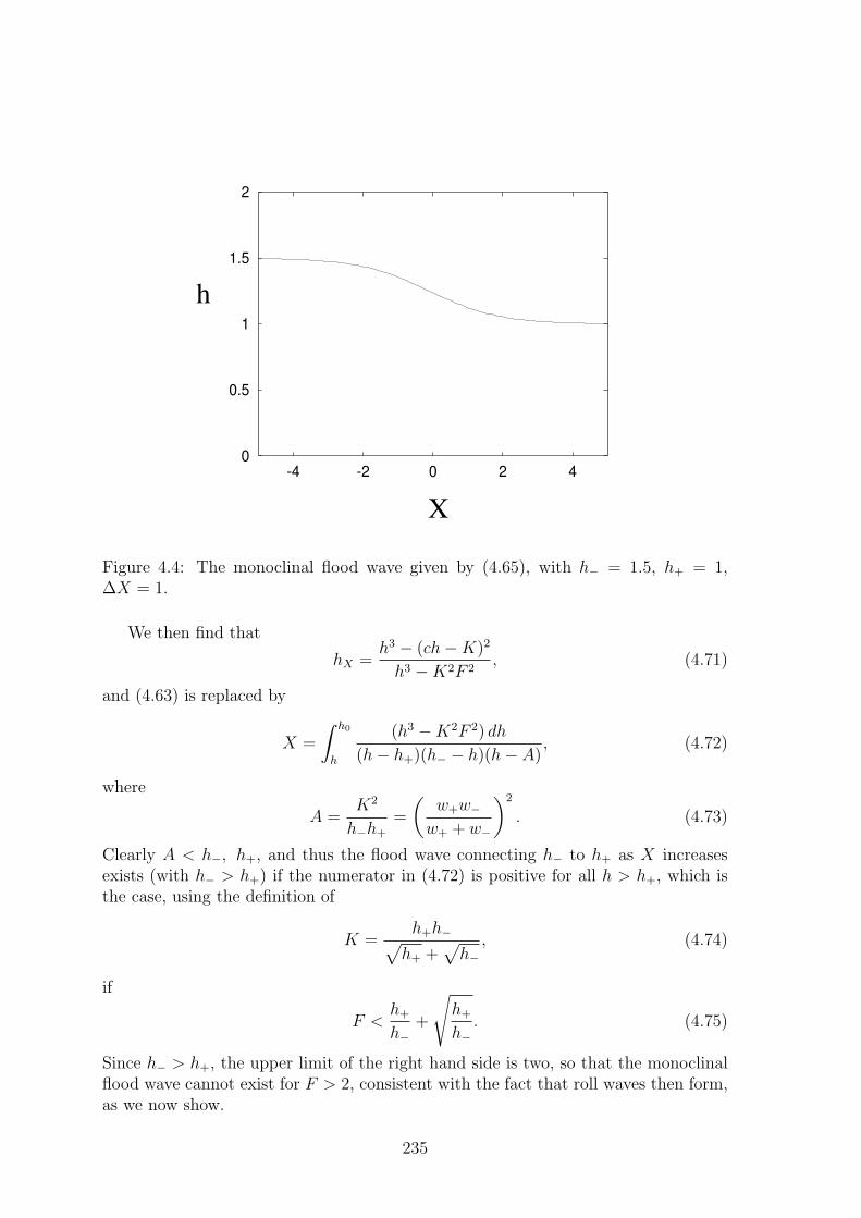
where d is the depth, and ∆d is the change in depth. Following a storm, if a river ofdepth two metres and bedslope 10−3 rises by a foot (thirty centimetres), the shockwidth is about thirteen kilometres: not very shock like! Figure 4.4 shows the form ofthe monoclinal flood wave (as given by (4.65)).

Although (4.57) is useful in indicating the diffusive structure of the long wavetheory, the above discussion of the monoclinal flood wave is strictly inaccurate, sincethe approximation in (4.56) breaks down on short scales. To see that the analysisstill holds, we can re-do the analysis on the full system (4.53). Adopting (4.58), wefind, approximately,

−chX + (uh)X = 0,

F 2(−cuX + uuX) = 1− u2

h− hX , (4.69)

with first integralch = K + uh, (4.70)

with K and c determined by (4.61) as before, noting that u± =√

h±, and thusu± = w±, as used in (4.63).

234

0

0.5

1

1.5

2

-4 -2 0 2 4

X

h

Figure 4.4: The monoclinal flood wave given by (4.65), with h− = 1.5, h+ = 1,∆X = 1.

We then find that

hX =h3 − (ch−K)2

h3 −K2F 2, (4.71)

and (4.63) is replaced by

X =

∫ h0

h

(h3 −K2F 2) dh

(h− h+)(h− − h)(h− A), (4.72)

where

A =K2

h−h+=

(w+w−

w+ + w−

)2

. (4.73)

Clearly A < h−, h+, and thus the flood wave connecting h− to h+ as X increasesexists (with h− > h+) if the numerator in (4.72) is positive for all h > h+, which isthe case, using the definition of

K =h+h−√

h+ +√

h−, (4.74)

if

F <h+

h−+

√h+

h−. (4.75)

Since h− > h+, the upper limit of the right hand side is two, so that the monoclinalflood wave cannot exist for F > 2, consistent with the fact that roll waves then form,as we now show.

235

4.4.4 Waves and instability

The monoclinal flood wave is one example of a river wave. More generally, we canexpect disturbances to a uniformly flowing stream to cause waves to propagate, andin this section we study such waves. In particular, we will find that if the basicflow is sufficiently rapid, then disturbance waves will grow unstably. Such wavesare commonly seen in fast flowing rivulets, for example on steep pavements duringrainfall, and even on car windscreens.

To analyse waves on rivers, we take the basic river flow as being (locally) constant,thus in (4.50) (with R = h)

u = h = 1, (4.76)

and we examine its stability by writing

u = 1 + v, h = 1 + H, (4.77)

and linearising. We obtain the linear system

Ht + Hs + vs = 0,

F 2(vt + vs) = −2v + H −Hs, (4.78)

whence

F 2

(∂

∂t+

∂

∂s

)2

v = −2

(∂

∂t+

∂

∂s

)v − vs + vss. (4.79)

Solutions v = exp[iks + σt] exist, provided σ satisfies

F 2(σ + ik)2 + 2(σ + ik) + ik + k2 = 0, (4.80)

orσ = −ik − 1 ± [1− ik − k2/F 2]1/2, (4.81)

where we writeσ = σ/F 2, k = k/F 2. (4.82)

There are thus two wave like disturbances. The possibility of instability exists, ifeither value of σ has positive real part. We define the positive square root in (4.81)to be that with positive real part. Specifically, we define

p + ikq =

{1− ik − k2

F 2

}1/2

, (4.83)

where we take p > 0; thus, the real and imaginary parts of σ are given by

σR = ± p− 1, − σI

k= 1∓ q, (4.84)

and the criterion for instability is that σR > 0, i. e., p > 1. In this form, the growthrate of the wave is σR/F 2, while the wave speed is −σI/k. From (4.83), we find

q = − 1

2p, L(p) ≡ p2 − k2

4p2= 1− k2

F 2. (4.85)

236

As illustrated in figure 4.5, L(p) is a monotonically increasing function of p, andtherefore the instability criterion p > 1 is equivalent to L(p) > L(1). Since p isdetermined by L(p) = 1− (k2/F 2), while from (4.85), L(1) = 1− (k2/4), we see thatinstability occurs if

F > Fc = 2. (4.86)

-4

-3

-2

-1

0

1

2

3

4

0 0.2 0.4 0.6 0.8 1 1.2 1.4 1.6 1.8 2

p

L

Figure 4.5: The function L(p) defined by (4.85), with k = 1.

Thus, for tranquil flow, F < O(1), the flow is stable. For rapid flow, F > O(1), itcan be unstable. The wave which goes unstable (when p = 1) propagates downstream,because its wave speed is 1 − q = 3

2 , and in fact the p > 0 wave always propagatesdownstream. The other wave, always stable, propagates downstream unless 1+q < 0,i. e., if and only if p < 1/2, or equivalently,

F < F− =2k

(3 + 4k2)1/2. (4.87)

Note that F− depends on k, and that 0 < F− < 1. Rewriting this inequality in termsof F and k, it is

F 2(1− F 2) >3

4k2, (4.88)

and upstream propagating waves are possible for short waves with k >√

3.We therefore have three distinct ranges for F :F > 2: two waves downstream, one unstable;1 < F < 2: two waves downstream, both stable;F < 1: stable waves can propagate upstream and downstream.

237

To go further than this requires a study of the nonlinear system (4.49). We see thatthe transition at F = 1 is associated with the ability of waves to propagate upstream.The transition at F = 2 is sometimes called Vedernikov instability, and is associatedwith the formation of downstream propagating roll waves.

4.5 Nonlinear waves

When F > 2, linear disturbances will grow, and nonlinear effects become importantin limiting their eventual amplitude. Because of the hyperbolic form of the equations,we might then expect shocks to form. To examine this hyperbolic form, we put

γ =1

F. (4.89)

The equations are thenht + (hu)s = 0,

ut + uus + γ2hs = γ2

[1− u2

h

], (4.90)

and they can be written in the form

∂

∂t

(hu

)+

(u hγ2 u

)∂

∂s

(hu

)=

0

γ2

[1− u2

h

]

. (4.91)

4.5.1 Characteristics

The analysis of characteristics for systems of hyperbolic equations is described in

chapter 1. The eigenvalues of B =

(u hγ2 u

)are given by

λ = u ± γh1/2, (4.92)

and the matrix P of eigenvectors and its inverse P−1 are given by

P =

( √h√

hγ −γ

), P−1 =

1

2γ√

h

(γ

√h

γ −√

h

). (4.93)

Comparing this with (1.69), we see that the integral

∫P−1 du =

∫

dh

2√

h+

du

2γdh

2√

h− du

2γ

=

√h +

u

2γ√h− u

2γ

(4.94)

is well-defined, and determines the characteristic variables (the Riemann invariants,so called because they are constant on the characteristics in the absence of the forcing

238

gravity and friction terms, as in shallow water theory). The equations can thus becompactly written in the characteristic form

[∂

∂t+ (u ± γ

√h)

∂

∂s

] [u ± 2γ

√h]

= γ2

[1− u2

h

]. (4.95)

Nonlinear waves propagate downstream if u/γh1/2 > 1, but one will propagate up-stream if u/γh1/2 < 1. This is consistent with the preceding linear theory (sinceu/γh1/2 is the local Froude number, i. e., the Froude number based on the local val-ues od velocity and depth). Because the equations (4.95) are of second order, simpleshock wave formation analysis is not generally possible. The equations (4.95) are verysimilar to those of gas dynamics, or the shallow water equations, and the equationssupport the existence of propagating shocks in a similar way.

4.5.2 Roll waves

There is a good deal of evidence that solutions of (4.90) do indeed form shocks, andwhen these are formed via the instability when F > 2, the resultant waves are calledroll waves. They are seen in steep flows with relatively smooth beds (and thus lowfriction), but this combination is difficult to find in natural rivers. It is found, however,in artificial spillways, such as that shown in figure 4.6, which shows a photograph ofroll waves propagating down a spillway in Canada. Roll waves can be found formingon any steep incline. Film flow down steep slopes during heavy rainfall will inevitablyform a sequence of periodic waves, and these are also roll waves; see figure 4.7. I usedto see them frequently at my daughter’s school, for example.

To describe roll waves, we seek travelling wave solutions to (4.90), in the formh = h(ξ), u = u(ξ), where ξ = s − ct is the travelling wave coordinate, c beingthe wave speed. Substitution of these into (4.90) yields the two ordinary differentialequations

−ch′ + (uh)′ = 0,

−cu′ + uu′ = 1− u2

h− γ2h′. (4.96)

The first equation has the integral

(u− c)h = −K, (4.97)

where K is a positive constant. The reason that it must be positive is that the positivecharacteristics (those with speed u+γh1/2) must run into (not away from) the shock,that is,

u+ + γh1/2+ < c < u− + γh1/2

− , (4.98)

where h+ and h− are the values of h immediately in front of and immediately behindthe shock. Hence

γh3/2+ < K < γh3/2

− . (4.99)

239

Figure 4.6: Roll waves propagating down a spillway at Lion’s Bay, British Columbia.The width of the flow is about 2 m, and the water depth is about 10 cm. Photographcourtesy Neil Balmforth.

Substitution of (4.97) into the second equation yields a single first-order equation foru, or h. We choose to write the equation for h, thus

h′ =h3 − (ch−K)2

γ2h3 −K2. (4.100)

As indicated in figure 4.8, we aim to solve this equation in (0, L), with h = h+ atξ = 0 and h = h− at ξ = L. The quantities involved in this equation and its boundaryconditions are L, c, h−, h+ and K, and these have to be determined. Solution of thedifferential equation (4.100) from 0 to L yields one condition,

L =

∫ h−

h+

γ2h3 −K2

h3 − (ch−K)2dh, (4.101)

which determines L in terms of the other quantities. Thus four extra conditions needto be specified to determine these.

There are two jump conditions to apply across the shock. These are conservationof mass, which we omit, as it is automatically satisfied by (4.97), and conservation ofmomentum, which has the form

c =

[hu2 + 1

2γ2h2

]+

−

[hu]+−. (4.102)

240

Figure 4.7: Laminar roll waves following rainfall at Craggaunowen, Co. Clare, Ireland.The water depth is a few millimetres and the wavelength of the order of twentycentimetres.

Simplification of this using (4.97) gives

[12γ

2h2 +K2

h

]+

−= 0. (4.103)

Evidently, consideration of the graph of 12γ

2h2 +K2

hshows that this determines h+

in terms of h−, for given K, see figure 4.9.We denote the critical value of h at the minimum in figure 4.9 as hm, thus

γ2h3m = K2; (4.104)

clearly we must have h− > hm and h+ < hm (this is also implied by (4.99)), thatis to say, the flow is subcritical behind the shock and supercritical in front of it. Inparticular, there is a value of ξ ∈ (0, L) with h = hm, and in order that the derivativein (4.100) remain finite, it is necessary that the numerator also vanish at this point.Since K > 0, this implies

chm −K =K

γ. (4.105)

We have added an extra quantity hm to the other unknowns L, h−, h+, K and c.To determine these six quantities, we have the four equations (4.101), (4.103), (4.104)and (4.105). This appears to imply that the roll waves described here form a two

241

L

u- , h-

u , u- , h-+ +h

c

Figure 4.8: Schematic form of roll waves.

parameter family, with (for example) the wavelength and wave speed being arbitrary.This is at odds with our expectation that a sensibly described physical problem willhave just the one solution. In order to understand this, we need to reconsider thehyperbolic form of the describing equations (4.90). A natural domain on which tosolve these equations is the semi-infinite real axis s > 0, in which case appropriateboundary conditions are to prescribe h and u on t = 0 and s = 0. The initialconditions are prescribed to represent the experimental start-up, and the boundaryconditions at s = 0 must represent the inlet conditions. The effect of the initialconditions is washed out of the system as the characteristics progress down stream,and the roll waves which are observed are determined by the boundary conditions ats = 0.

Of course, these inlet conditions are not generally consistent with a periodic trav-elling wave solution, but we would expect that prescribed values of u and h at theinlet would provide the extra two parameters to fix the solution precisely. One suchparameter is easy to assess. Because mass is conserved, the mean volume flux mustbe equal to that at the inlet, and by choice of the velocity and depth scales, we cantake the volume flux to be one, whence

1

L

∫ L

0

(ch−K) dξ = 1. (4.106)

It is not as obvious how to provide the other recipe, because the mean momentumflux is not conserved downstream; its value at the inlet does not tell us its valuedownstream. This is because of the gravity and friction terms. However, it is thecase that these terms must balance on average, that is to say,

∫ L

0

(h− u2) dξ = 0; (4.107)

this actually follows by integrating the momentum equation (written in conservationform) over a wavelength. The momentum advection and pressure gradient termsvanish because of (4.103), leaving (4.107). This appears to give a final condition toclose the system: but it does not, as (4.107) actually reduces to (4.103) when the

242

0

2

4

6

8

10

0 0.5 1 1.5 2 2.5 3 3.5 4

h

hm

+ -h

Figure 4.9: Supercritical and subcritical values of h across a shock: graph of 12γ

2h2 +K2/h, γ = K = 1.

integration is carried out. An appropriate final condition is not easy to determine; weprovide some further discussion below. Before that, we reduce the conditions aboveto a simpler form.

We rewrite the relations (4.101), (4.103), (4.104), (4.105) and (4.106) using hm asthe defining parameter, and putting

h+ = hmφ+, h− = hmφ−; (4.108)

then we have K and c given by

K = γh3/2m , c = h1/2

m (1 + γ), (4.109)

and L, φ+ and φ− are determined, after some algebra, by

L = γ2hm

∫ φ−

φ+

(φ2 + φ + 1) dφ

(φ− γ)2 − γ2φ,

1 =γ2h5/2

m

L

∫ φ−

φ+

(φ2 + φ + 1){φ + γ(φ− 1)} dφ

(φ− γ)2 − γ2φ,

[12φ

2 +1

φ

]+

−= 0, (4.110)

where we have taken Q = 1 in (4.106). The second of these can be written indepen-

243

dently of L as

q =

∫ φ−

φ+

(φ2 + φ + 1){φ + γ(φ− 1)} dφ

(φ− γ)2 − γ2φ∫ φ−

φ+

(φ2 + φ + 1) dφ

(φ− γ)2 − γ2φ

, (4.111)

where

q =1

h3/2m

. (4.112)

The profile of φ is given by the scaled version of (4.100), which is

φ′ =(φ− γ)2 − γ2φ

γ2hm(φ2 + φ + 1). (4.113)

The numerator must be positive, and since φ = 1 for some ξ, a necessary conditionfor this to be true is that γ < 1/2. In terms of the Froude number, this is F > 2,which is the condition under which the roll wave instability occurs in the first place.This nicely suggests that the roll waves bifurcate as a non-uniform solution from thesteady state at F = 2.

It is apparent from the above discussion that the crux of the determination of theroll wave parameters is the solution of (4.110)3 and (4.111) for given positive q. If φ+

and φ− can be found for any such q, then they can be found for any hm, after whichL, K and c follow directly from (4.109) and (4.110)1.

To find the solutions of (4.110)3 and (4.111), we note that φ+ and φ− are uniquelydefined in terms of the ordinate of the graph in figure 4.9; in fact, for any φ+ ∈ (0, 1),(4.110)3 gives the explicit solution

φ− = 12

[−φ+ +

{φ2

+ +8

φ+

}1/2]

; (4.114)

then (4.111) gives q = q(φ+; γ). The other constants are then given explicitly by(4.109), (4.110)1 and (4.111), and in particular, if we define

N(φ+) =

∫ φ−

φ+

(φ2 + φ + 1){φ + γ(φ− 1)} dφ

(φ− γ)2 − γ2φ,

D(φ+) =

∫ φ−

φ+

(φ2 + φ + 1) dφ

(φ− γ)2 − γ2φ, (4.115)

(thus q = N/D), then using

hm =

(D

N

)2/3

, (4.116)

we have

L =γ2D5/3

N2/3, c =

(1 + γ)D1/3

N1/3, K =

γD

N. (4.117)

244

The equations (4.114), (4.116) and (4.117) determine φ−, hm, L, c and K in termsof φ+. From these we can find h− and h+. Thus it is convenient in computing theone parameter family of wave solutions to use φ+ as the parameter.

In figures 4.10–4.12 we plot the wave height ∆h = hm(φ− − φ+), wavelength Land speed c (all dimensionless) as a function of the parameter φ+, for various valuesof the Froude number F .

h∆

0

2

4

6

8

10

0 0.2 0.4 0.6 0.8 1

γ = 0.1

γ = 0.2

γ = 0.4

φ+

Figure 4.10: Graphs of ∆h = h− − h+ as a function of φ+ for γ = 0.1 (F = 10),γ = 0.2 (F = 5) and γ = 0.4 (F = 2.5). The asterisks mark the ends of the curves atφ+ = α+.

A feature of figure 4.10 is the termination of the curves at a finite value. Theintegrals which define N and D in (4.115) can be explicitly evaluated. If we definethe two (positive) roots of (φ− γ)2 − γ2φ = 0 to be

α± =γ

2

[2 + γ ± {γ2 + 4γ}1/2

], (4.118)

thus α+ > α− > 0, then we restrict φ+ > α+ so that φ′ > 0 in (4.113). Considerationof N and D then shows that

D = −A ln(φ+ − α+) + O(1), N = −C ln(φ+ − α+) + O(1) (4.119)

as φ → α+. From this it follows that q → q+ as φ → α+, where q+ = C/A, and isgiven explicitly by

q+ = (1 + γ)α+ − γ. (4.120)

These termination points are marked by asterisks at the end of the curves in figure

4.10. Because q = q+ + O

(1

− ln(φ+ − α+)

), the slope of the curves is infinite at

245

φ+

γ = 0.1

γ = 0.2

γ = 0.4

0

0.5

1

1.5

2

0 0.2 0.4 0.6 0.8 1

L

Figure 4.11: Dimensionless wavelength L in terms of φ+ for γ = 0.1 (F = 10), γ = 0.2(F = 5) and γ = 0.4 (F = 2.5). The curves do not terminate, since L ∼ − ln[φ+−α+]as φ+ → α+.

0

1

2

3

0 0.2 0.4 0.6 0.8 1

φ+

γ = 0.1

γ = 0.2 γ = 0.4

c

Figure 4.12: Wave speed c in terms of φ+. The asterisks mark the ends of the curves

at φ+ = α+, c = c+ =1 + γ

q1/3+

.

246

0

1

2

3

0 2 4 6 8 10

γ = 0.1γ = 0.2

γ = 0.4

c

L

Figure 4.13: Wave speed c as a function of L, for γ = 0.1, γ = 0.2 and γ = 0.4. Theshort dashed lines at the right ordinate indicate the corresponding asymptotes c+ forγ = 0.1 and γ = 0.2 and γ = 0.4 at the respective values c+ = 2.9717, 2.1495, 1.6216.

these points. (This also makes it hard to draw the figures. To get within 0.02 of q+,for example, we can expect to have to take φ+ − α+ ≈ exp(−50) ≈ 10−22 !)

As φ+ → 1, then also φ− → 1, and hence both N and D are O(1). Directconsideration of (4.115) shows that q → 1 as φ+ → 1. As a consequence of theselimiting behaviours, L → 0 and c is finite as φ+ → 1, while L → ∞ as φ+ → α+,but c tends to a finite limit just as q does. As shown in figures 4.10–4.12, all threequantities vary monotonically between φ+ = α+ and φ+ = 1, and consequently c is amonotonically increasing function of L, which tends to a limit c+ as L→∞, where

c+ =(1 + γ)

q1/3+

. (4.121)

This is shown in figure 4.13. Analysis of the limit φ+ → α+ shows that c = c+ +O(1/L) as L → ∞ (question 4.15), and evidently the approach to the limit is slow,particularly at low γ (high Froude number).

Wavelength selection and boundary conditions

Although it is convenient to compute the properties of the roll waves using the pa-rameter φ+, it is more natural to use the wavelength L as the single parameter. Theissue remains how this is selected. This seems to be an open problem, on which weoffer some comments, though little further insight.

The first thing to note is that the hyperbolic St. Venant equations (4.90) requiretwo initial conditions at the inlet s = 0 if the Froude number F > 1. If we imagine

247

flow from a vent below a dam, for example, it is easy to see that prescription of both hand hu (and thus u) can be effected, by having a vent opening of a prescribed height,and adjusting the dam height to control mass flow. From a mathematical point ofview, precisely steady inlet conditions h = u = 1 lead to uniform downstream flow,provided the St. Venant equations apply precisely. Thus we can see that it is onlythrough the prescription of a time varying inlet velocity, for example, that roll wavescan develop downstream. For example, we might prescribe inlet conditions

h = 1, u = 1 + λ cos ωt at s = 0, (4.122)

where λ ' 1. We would then infer that the resulting periodic solution would havefrequency ω, and this would prescribe the ratio

L

c= ω, (4.123)

which would provide the final prescription of the solution. Consulting figure 4.13, wecan see that (4.123) would indeed determine a unique value of L.

More generally, we might suppose u(0, t) to be a polychromatic, perhaps stochasticfunction. We might then expect the wavelength selected to be that of the most rapidlygrowing mode. Consultation of (4.85), however, indicates that for F > 2, p and thusReσ is an increasing function of wavenumber k, with p → F as k → ∞. Thisunbounded growth at large wave number is suggestive of ill-posedness, and in anycase is certainly not consistent with the apparent observation that long wavelengthroll waves are in practice selected.

A final consideration, and perhaps the most practical one, is that wavelengthselection may take place at large times through the interaction of neighbouring wavecrests. Larger waves move more rapidly (c is an increasing function of ∆h if we plotone in terms of the other), and therefore larger waves will catch smaller ones. Thisprovides a coarsening effect, whereby smaller waves can be removed by larger ones.Since ∆h is also an increasing function of L, this coarsening does indeed lead tolonger waves. The process should be limited by the fact that very long (and thusflat) waves will be subject to the same Vedernikov instability as is the uniform state.4

If we supposed that wavelength varied slowly from wave to wave, we can see thebeginnings of a kind of nonlinear multiple scales method to describe the evolution ofwavelength as a function of space and time. It is less easy to see how to incorporatethe generation of new waves in such a framework, however, and this problem remainsopen for investigation.

The spectre of ill-posedness described above raises the related issue of how toprescribe the correct boundary conditions for the St. Venant equations. The reasonthere is an issue is that the equations require two upstream boundary conditions ifF > 1, but one upstream and one downstream condition if F < 1. This makes nosense, insofar as the boundary conditions should be prescribed independently of thesolution. A resolution of this conundrum lies in the realisation that the formation

4This observation is due to Neil Balmforth.

248

of shocks in the hyperbolic system suggests the presence of a missing diffusive term,and this takes the form of a turbulent eddy viscous term.

In our discussion of the basal friction term (4.5), we assumed only the transverse

Reynolds stress −ρu′w′ ≈ µT∂u

∂zwas significant. The longitudinal Reynolds stress

−ρu′2 ≈ µT∂u

∂xis small, but provides a crucial diffusive term

∂

∂x

(µT A

∂u

∂x

)(4.124)

to be added to the right hand side of (4.43). Following (B.9) in appendix B , wesuppose

µT = ρεT [u]d, (4.125)

and this leads to the corrective term

εT F 2S1

A

∂

∂x

(A

∂u

∂x

)(4.126)

to be added to (4.49)2. Correspondingly, the equations (4.90) are modified to

ht + (hu)s = 0,

ut + uus + γ2hs = γ2

[1− u2

h

]+

κ

h

∂

∂s

(h∂u

∂s

), (4.127)

whereκ = εT S ' 1. (4.128)

A typical value of κ is ∼ 10−5.Because κ is small, it can be expected to provide a shock structure for the shocks

we have described. In addition, the extra derivative suggests that an extra boundarycondition for the system (4.127) needs to be prescribed. Most obviously, this is atthe outlet, where the river meets the sea. The most obvious such condition might beto prescribe h, or perhaps hx, but it is more likely that one should prescribe

u = 0 at s = 1, (4.129)

indicating the flow of the river into a large reservoir. In any event, the extra conditionat the outlet, together with the diffusive term (4.124, can explain the difference inthe solutions when F <

> 1. The characteristics of (4.90) are the sub-characteristics of(4.127), and the appropriate pair of conditions to apply for (4.90) is determined bythe correct way of determining the singular approximation when κ→ 0.

However, this really sheds no further light on the issue of roll wave length selection.When F > 2, clearly two conditions are appropriate at s = 0, but how these conspireto select the wavelength is unclear.

249

Figure 4.14: The Severn bore. This is a famous photograph apparently from 1921,when there were no bystanders, and certainly no surfers. Reproduced from Pugh(1987). The photograph first appears in the book by Rowbotham (1970), where MrC.W.F. Chubb is acknowledged as the photographer, and is reprinted here courtesyof David and Charles, Newton Abbot.

4.5.3 Tidal bores

A bore on a river is a shock-like wave which travels upstream, and it occurs becauseof forcing at the mouth of the river due to tidal variation in sea level. In England thebest known example is the Severn bore, which occurs because of the very high tidalrange in the Severn estuary. Large crowds come to view the bore, which manifestsitself as a wall of water about a metre high advancing up river at a speed of somefour to five metres a second. Figure 4.14 shows a photograph of the Severn bore.Bores occur on certain rivers due to a confluence of factors. The tidal range has to bevery large, and this can be caused by tidal resonance in an estuary; in addition, theriver must narrow dramatically upstream, so that the estuary acts like a funnel. Thewave then forms because the rapidly rising water level in the estuary causes a largeupstream water flux, and with a sufficiently large funnelling effect, a shock wave willbe formed. Bores occur all over the world, for example in the Amazon, the Seine,the Petitcodiac river which flows into the Bay of Fundy, and the Tsien Tang river inChina. Where they occur, they are spectacular, but relatively few rivers have them,because of the severity of the necessary conditions for their formation.

Figure 4.16 shows the geometry of the Severn river and estuary. The bore formsnear Sharpness, and is best viewed at various places further upstream, notably Min-sterworth and Stonebench, where public access is available. Figure 4.17 shows aprofile of the river during passage of a bore. There are certain features evident in this

250

Figure 4.15: The Severn bore, viewed from the air in a microlight aircraft by MarkHumpage. The image is copyright Mark Humpage, and is reproduced with his per-mission. For other photographs, see http://www.markhumpage.com. The undularnature of the bore is very clearly visible (as are the relentless surfers).

figure which are relevant when we formulate a model. The river depth at low stageis about a metre, whereas the tidal range is much greater than this. In the Severnestuary, it can be 14.5 metres, and at Sharpness, it is 9 metres in the figure. Theother feature of importance is the apparent alteration in the bedslope as the estuaryis approached. As an idealisation of this, figure 4.18 shows the basic geometry of ariver–estuary system, which we can use to explain bore formation.

The river in figure 4.18 flows into a tidal basin, where the water level fluctuatestidally with a period of slightly more than twelve hours. Such fluctuations cause theriver/estuary boundary point to migrate back and forth. In particular, approachinghigh tide this point moves upstream. The idea behind bore formation is that if theupstream velocity of this boundary is faster than the upstream characteristic wavespeed,5 a smooth wave cannot occur, and a shock must form, as indicated in figure4.18.

We want to study this phenomenon in the context of the St. Venant equations(4.49), where for a wide channel, we choose the hydraulic radius and cross sectional

5We assume the Froude number F is less than one at low stage, which is the realistic condition;in that case, one wave travels upstream. If F > 1, a standing wave would form at the boundary.

251

Avonmouth

BristolChannel

River Wye

Severn Bridge

Sharpness

Framilode

Minsterworth

Stonebench

Gloucester

Maisemore

10 km

Figure 4.16: A sketch map of the river Severn.

Framilode

Minsterworth

Stonebench

Maisemore

ebbing high flowing bore

low water

0 3020 40 km10

9 m

0 m

Newnham

The HockSharpness

Figure 4.17: Profile of the Severn during passage of a bore. Note that high wateroccurs someway below the bore (the tide continues to come in after the passage of thebore), but that the tide near Sharpness already starts to ebb before the bore reachesMaisemore.

252

river

estuary

tidalvariation

bore

s

s = 0

s = 1

Figure 4.18: Idealised (and highly exaggerated) river basin geometry.

area to beR = h, A = wh, (4.130)

where w is the width, and is taken to be a prescribed function of s. The phenomenonof concern occurs over the length of the river, so that long wave theory is appropriate.From figure 4.17, a suitable length scale is of the order of 45 km, where the length scaleused in writing (4.49) is d/ sin α, and is 2 km if we take d = 2 m and S = sin α = 10−3.If we take a typical velocity upstream as 2 m s−1, then the corresponding time scaleis 103 s, or 15 minutes, and the Froude number is about 0.3. The scale up in distanceis thus of order 22, while that in time to the half-period of tidal oscillations is similar.This suggests that we rescale both time and space as

t ∼ 1

ε, s ∼ 1

ε, (4.131)

where a plausible value of ε may be of order 0.05. In this case (4.49) can be writtenin the form (where now, because u will be negative during inflow, we take the frictionterm in the corrected form ∝ |u|u)

wht + (wuh)s = 0,

εF 2(ut + uus) = 1− |u|uh− εhs, (4.132)

or equivalently in the form

ε

[±F

∂

∂t+ (√

h ± Fu)∂

∂s

] [2√

h ± Fu]

= 1− |u|uh∓ εFw′

√hu

w, (4.133)

253

which shows explicitly that the characteristic wave speeds are

±√

h

F+ u, (4.134)

as we found before. Finally, we wish to study the situation shown in figure 4.18, wherethe tidal range is significantly larger than the river depth. The simplest choice is tosuppose the tidal amplitude is also O(1/ε), so that appropriate boundary conditionsfor (4.132) are

wuh = 1 at s = 0,

h =H1(t)

εat s = 1, (4.135)

representing a constant upstream volume flux, and a prescribed tidal range.The assumption that ε' 1 allows us to solve (4.132) asymptotically. The solution

has two parts, river and estuary, joined at a front which we denote by s = sf .Upstream, for s < sf , the flow is quasi-stationary, and we have, to leading order,

wuh ≈ 1, 1− u|u|h≈ 1, (4.136)

whenceu ≈ w−1/3, h = w−2/3. (4.137)

The steady solution of (4.132) is appropriate, because the sub-characteristic wavepropagates downstream, and after any initial transient, the upstream boundary con-dition leads to a steady flow.

Downstream, for s > sf , we write

h =H

ε, (4.138)

so that

wHt + (wuH)s ≈ 0,

1−Hs ≈ 0 (4.139)

(the surface is flat); from this we have

H ≈ s− 1 + H1(t), (4.140)

and from this there follows

u ≈−H1

∫ s

sf

w ds

wH, (4.141)

where we choose the integration constant for matching purposes at sf . Also to matchthe solution to that in s < sf , we need to take

sf = 1−H1. (4.142)

254

Transition region

At the front, we define

s = sf + εX, sf = c, wf = w [sf (t)] ; (4.143)

then to leading order we have

−cwfhX + (wfhu)X = 0,

F 2(u− c)uX = 1− u|u|h− hX , (4.144)

with boundary conditions

h→ h− = w−2/3f , u→ u− = w−1/3

f as X → −∞,

h ∼ X, u ∼ c as X →∞, (4.145)

in order to match to the upstream and downstream solutions. Note that this transitionregion, like that for the monoclinal flood wave, is mediated by the full St. Venantequations, but without a diffusive term. Only the conditions on h in (4.145) arenecessary, those on u following automatically. A first integral of the mass conservationequation (4.144)1 gives

(u− c)h = K =[w−1/3

f − c]w−2/3

f , (4.146)

and from this we find

hX =h3 − |K + ch|(K + ch)

h3 −K2F 2. (4.147)

This can be compared with (4.100). The difference in the present case is that c andK in (4.143) and (4.146) are given, and the question is only whether a solution exists

joining h = h− = w−2/3f upstream to the downstream solution h ∼ X. Note that as

X → −∞, K + ch→ w−1f , so that h→ w−2/3

f can consistently be satisfied.Let us suppose that the tide is coming in, thus c < 0. We suspect that a smooth

solution in the transition region may not be possible if−c is greater than the upstreamwave speed. Using (4.134) and (4.145), this condition can be written in the form

−c > w−1/3f

(1

F− 1

)(4.148)

(assuming F < 1). If we suppose that the opposite inequality holds, i. e., −c <

w−1/3f

(1

F− 1

), then a little algebra shows that this is precisely the criterion that

h− = w−2/3f > (KF )2/3, (4.149)

i. e., the denominator of (4.147) is positive. To see that there is a solution of thisproblem in this case, we need to show that the numerator of the right hand side(4.147) is also positive, for then h will increase indefinitely as required.

255

The numerator, N , is given by

N ={h3 − w−2

f

}−

{∣∣∣w−1f + c

(h− w−2/3

f

)∣∣∣[w−1

f + c(h− w−2/3

f

)]− w−2

f

}. (4.150)

Both expressions in curly brackets are zero when h = h− at X = −∞; for h slightlygreater than h−, the left curly bracketed expression is positive, while the right curlybracketed expression decreases, since c < 0. The numerator is thus positive forh− h− small and positive, and remains so. From this it follows that a solution of the

transition problem exists if −c < w−1/3f

(1

F− 1

), and thus a bore will not form.

It remains to be shown that no solution exists if the opposite inequality, (4.148),holds. In this case the denominator of the right hand side of (4.147) is initiallynegative. As before, the numerator is positive if h > h−, and equivalently negative ifh < h−, thus implying hX < 0 if h > h−, and hX > 0 if h < h−. This means solutionsof (4.147) can only approach h− as X → ∞, and no transition solution exists. Thissuggests another form of solution, one in which a discontinuity forms at the criticalcondition

−sf = w(sf )−1/3

(1

F− 1

), (4.151)

and thereafter propagates upstream as a shock front. This is the bore. Figure 4.19shows a schematic illustration of the criterion (4.151) for bore formation.

Propagation of the bore

The outer river and estuary solutions (4.137), (4.140) and (4.141) remain valid afterthe formation of a shock, but the transition region is replaced by a shock at sf , wherethe values of h− and u− (given by (4.137) with w = wf ) jump (up) to values h+ andu+, which have to be determined along with sf . Initially h+ and u+ are O(1), andwe anticipate that this remains true; in this case sf is still given by

sf = 1−H1 + O(ε); (4.152)

the location of the bore is essentially determined by the tidal range. Jump conditionsof mass and momentum across the developing bore then imply that the bore speedsf = c satisfies

c =[hu]+−[h]+−

=12 [h

2]+− + F 2[hu2]+−[hu]+−

, (4.153)

and these two relations serve to determine h+ and u+, since c = −H1.

Shock structure

We can use the transition equations (4.144), modified by the addition of the diffusiveterm in (4.127), to study the shock structure of the bore. The equations then takethe form

−cwfhX + (wfhu)X = 0,

256

1

−.

sf

sf

sfwf

_1/ 3 _1F

_ 1)

._

bore

no bore

(

Figure 4.19: Bore formation occurs for large tides and rapidly widening rivers withreasonably sized Froude numbers. If the tide oscillates sinusoidally and the river slopeis constant, then the front position sf will trace an ellipse as shown in the (sf , sf )plane. For a funnel-shaped river, the width w decreases as sf decreases, so that(

1

F− 1

)w−1/3 is a decreasing function of sf , as shown. Bore formation therefore

occurs according to (4.148) for the solid tidal curve, but not for the smaller amplitudedotted one.

F 2(u− c)uX = 1− u|u|h− hX +

κF 2

h

∂

∂X

(h

∂u

∂X

), (4.154)

and the boundary conditions are still (4.145). The difference with the precedinganalysis is that when a bore forms, we expect the diffusive term to act as a singularperturbation which allows the matching of two distinct outer solutions through aninterior shock (the bore). Writing

u = c +K

h, (4.155)

we find that h satisfies

∂h

∂X=

h3 − |K + ch|(K + ch)

h3 −K2F 2− κF 2Kh2

h3 −K2F 2

∂

∂X

[1

h

∂h

∂X

]. (4.156)

As discussed before (4.151), the only way h can approach h− as X → −∞ inbore-forming conditions is if the outer solution (where κ = 0) in X < 0 is

h ≡ h−, X < 0. (4.157)

We suppose that h jumps through the shock to a value h+ > h−. According to theargument following (4.150), the numerator of (4.147) for the outer solution in X > 0

257

is then positive, and so, providing h3+ > K2F 2, the outer solution for h will increase

monotonely from h+, and h ∼ X as X → ∞. It only remains to show that a shockstructure exists connecting h− to h+ > (KF )2/3.

Supposing without loss of generality the shock to be at X = 0, we define

X = κKF 2ξ (4.158)

(noting that K > 0), so that to leading order (4.156) becomes

∂h

∂ξ= − h2

h3 −K2F 2

∂

∂ξ

[1

h

∂h

∂ξ

]. (4.159)

Integrating this, we find

∂h

∂ξ= −h

[12

(h2 − h2

−)

+ K2F 2

(1

h− 1

h−

)]. (4.160)

Consideration of the right hand side of this equation shows that if h3− < K2F 2, then

−h′

his zero at h = h−, negative for h > h− until it becomes positive for large h.

Thus there is one further zero of h′ at h+ > h−, and h′ > 0 between these two values,always assuming that h3

− < K2F 2, which is guaranteed by (4.149). Thus the shocklayer structure takes h monotonically from h− to h+, given by

12

(h2

+ − h2−)

= K2F 2

(1

h−− 1

h+

), (4.161)

and it only remains to check that h+ > (KF )2/3, so that the outer solution to (4.147)

in X > 0 does indeed increase as X → ∞. This is clear from the definition of −h′

h

given by (4.160), which shows that −h′

his a convex upwards function G(h), and in

particular shows that G′(h+) > 0. Since from (4.159),

G′(h) =h3 −K2F 2

h2, (4.162)

we can deduce that indeed h+ > (KF )2/3.This analysis shows that in bore-forming conditions, the diffusive term in (4.154)

does indeed allow a shock structure to exist, and this describes what is known as aturbulent bore, appropriate at reasonably large Froude numbers. The Severn boreshown in figure 4.15 is an example of an undular bore, appropriate at lower Froudenumbers, and consisting of an oscillatory wave train. The St. Venant equations donot appear to be able to describe this kind of bore, where the oscillations have awavelength comparable to the depth, and the vertical velocity structure may need tobe considered in attempting to model it. This is discussed further below.

258

4.6 Notes and references

A preliminary version of the material in this chapter is in my own book on modelling(Fowler 1997), although with much less detail than presented here. The generalsubject of river flow is treated in its contextual, geographical aspect by books onhydrology, such as those of Chorley (1969) or Ward and Robinson (2000). Ward andRobinson’s book, for example, deals with precipitation, evaporation, groundwaterand other topics as well as the dynamics of drainage basins, but is less concernedwith detailed flow processes in rivers. For these, we turn to books on hydraulics, suchas those by French (1984) or Ven te Chow (1959). A nice book which bridges thegap, and also includes discussion of sediment transport and channel morphology andpattern, is that by Richards (1982).

Roll waves

Flood waves and roll waves have been discussed from the present perspective byWhitham (1974). The linear instability at Froude number greater than two wasanalysed by Jeffreys (1925), and the finite amplitude form of roll waves was describedby Dressler (1949), whose presentation we follow here. The book by Stoker (1957)gives a nice discussion, as well as a useful photograph of roll waves on a spillway inSwitzerland. The eddy viscous diffusive term in (4.127) was added by Needham andMerkin (1984). Balmforth and Mandre (2004) provide a thorough review, and alsoprovide a discussion of the mechanics of wavelength selection. They also, followingYu and Kevorkian (1992), provide a weakly nonlinear model for roll wave evolutionwhen F − 2 ' 1; a strongly nonlinear model would be more relevant at higher F .Their experiments are consistent with the idea that the form of the inlet condition isinstrumental in determining the roll wavelength.

Tidal bores

The effect of tidal variations on river flow is discussed by Pugh (1987); in particular,he describes the phenomenon of the river bore. Another useful little book is thatby Tricker (1965). The literature on bores seems to be rather sparse, although thephenomenon itself has been well known for a (very) long time. Chanson (2005) refersto the fact that the mascaret of the Seine river in France was documented in the ninthcentury A.D. Lord Rayleigh, then president of the Royal Society, writes down thejump conditions for the bore velocity over a hundred years ago (Rayleigh 1908). Thereis a very informative article by Lynch (1982), prior to which the principal analysis isthat of Abbott and Lighthill (1956), who analyse the St. Venant equations, and applytheir results to the Severn bore. The presentation is extremely opaque, however. Thelittle book by Rowbotham (1970) is a gem, and has many other striking photographsbesides that shown in figure 4.14.

More recently, there has been an upsurge of interest in modelling bores. Su et al.(2001) construct a numerical model of the turbulent bore of the Hangzhou Gulf andQiantangjiang river in China using the St. Venant equations. In a number of papers,

259

Chanson and co-workers have studied the dynamics of undular bores (Wolanski etal. 2004, Chanson 2005), both observationally and experimentally. Chanson (2009)reviews the observational and experimental literature, with numerous illustrations.

In order to obtain an oscillatory wave train (such as one also finds in capillarywaves), it seems that a higher derivative term in (4.160) might be necessary, eitheras hξξξ or from a term uXXX in (4.154). Such terms are commonly found in higherorder approximations to water wave equations, as for example in the Korteweg–deVries equation. To get a flavour of such an analysis, we consult the derivation of theKorteweg–de Vries equation by Ockendon and Ockendon (2004, pp. 106 ff.). Revertingto dimensional coordinates, their derivation of the Korteweg–de Vries equation takesthe form, assuming a backwards travelling wave,

ut + . . . =

√gd d2

6usss. (4.163)

If we simply suppose that such a term can be added to the St. Venant equation, then,using the scales in (4.48), the St. Venant equations (4.50) or (4.127) become

wht + (wuh)s = 0,

F 2(ut + uus) + hs = 1− |u|uh

+κF 2

h

∂

∂s

(h∂u

∂s

)+ 1

6FS2 usss. (4.164)

Repeating the shock structure analysis, (4.156) is replaced by

−16FKS2

(1

h

)

XXX

+ κF 2Kh2

(hX

h

)+ P (h)hX −N(h) = 0, (4.165)

whereP (h) = h3 −K2F 2, N(h) = h3 − |K + ch|(K + ch) (4.166)

(N(h) is the numerator in (4.147) discussed following (4.150)).We write

h = h−φ, N = h3−n(φ), P = h3

−p(φ), c = −√

h−V, (4.167)

whence (4.145) and (4.146) imply

K = h3/2− (1 + V ), (4.168)

and hence

n(φ) = φ3 − |1 + V − V φ|(1 + V − V φ), p(φ) = φ3 − (1 + V )2F 2. (4.169)

Lastly we putX = h−Z. (4.170)

Then (4.165) becomes

−δ

(1

φ

)

ZZZ

+ βφ2

(φZ

φ

)

Z

+ p(φ)φZ − n(φ) = 0, (4.171)

260

1

2

3

-1 -0.5 0 0.5 1

X

h

Figure 4.20: Model of a turbulent bore. Solution of (4.165) in the form (4.171), usingvalues F = 1.5, V = 0, β = 0.1, δ = 0.01. The time step used is 10−5, and the plottakes h− = 1 in its scales for X and h.

where

δ =F (1 + V )S2

6h11/2−

, β =κF 2(1 + V )

h3/2−

, (4.172)

and both are small.The boundary conditions for φ are that

φ→ 1 as Z → −∞, φ ∼ Z as Z →∞. (4.173)

Figures 4.20 and 4.21 show numerical solutions of the transition equation (4.171)for two different values of β. The first corresponds to a relatively high value of β,when δ is sufficiently small to be ignored, and the preceding shock structure analysis(following (4.154)) is valid. Formally this requires δ ' β2.

At lower values of β, however, it is inadmissible to neglect the third derivativeterm. To analyse what happens in this case, write

Z =√

δζ, (4.174)

and define

µ =β√δ. (4.175)

Assuming δ ' 1, we can neglect the term in n within the transition zone, so that

−(

1

φ

)

ζζζ

+ µφ2

(φζ

φ

)

ζ

+ p(φ)φζ ≈ 0. (4.176)

261

1

2

3

4

-1 -0.5 0 0.5 1

h

X

Figure 4.21: Model of an undular bore. Solution as for figure 4.20, except thatβ = 0.001.

The turbulent bore is regained if µ- 1. For the case µ <∼ 1, define

ψ = 1− 1

φ, (4.177)

whence

ψ′′′ +µ

(1− ψ)2

{ψ′

(1− ψ)

}′

+ p

(1

1− ψ

)ψ′

(1− ψ)2= 0. (4.178)

Suppose first that µ is small; then a first integral of (4.178) with µ = 0 is

ψ′′ + W ′(ψ) = 0, (4.179)

where

W ′(ψ) =

∫ 11−ψ

1

p(φ) dφ, W (0) = 0. (4.180)

Integrating and changing the order of integration, we can write

W (ψ) =

∫ 11−ψ

1

[ψ −

(1− 1

φ

)]p(φ) dφ. (4.181)

As a function of ψ, W (0) = W ′(0) = 0, and (since p(1) < 0, equivalent to thebore-forming condition (4.148)) W ′′(0) < 0; thus W is negative for small ψ > 0.

Since W ′′(ψ) =p(φ)

(1− ψ)2, and p is an increasing function of φ, we see that W reaches

a negative minimum, and thereafter increases, tending towards ∞ as ψ → 1 andφ→∞.

262

(4.179) is the equation of a nonlinear oscillator, and shows that φ increases fromzero at Z = −∞, and then oscillates about the minimum of W . In fact with µ = 0,there would be precisely one oscillation, with φ returning to zero at Z = +∞. Thisdoes not happen for two reasons. The term in µ is a damping term (this is clear in(4.176) if the coefficient φ2 is ignored; alternatively one can view (4.176) as a dampedoscillator for ψ), so that the oscillations are damped towards the minimum of W ; andthe small term in n in (4.171) causes a drift upwards in φ towards the outer solution

given by φZ ≈n(φ)

p(φ). Both these features can be seen in figure 4.21.

Although in this context, the introduction of the long wave dispersive term usss in(4.164) is merely suggestive, it does show that such a term can produce the undularbore seen in practice at relatively low Froude number. The classical approach is givenin the paper by Peregrine (1966), who simply writes down as a model the Benjamin–Bona–Mahony (BBM) equation, also called the regularised long wave (RLW) equa-tion, which in essence introduces a term usst in (4.164) in place of usss. The BBMequation was (re-)introduced by Benjamin et al. (1972) as a suggested improvementto the Korteweg–de Vries (KdV) equation, on the basis that it has better regularityproperties. Specifically, the dispersion relation for modes eik(s−ct) is c = 1 + k2 for

the linearised KdV equation ut + us = usss, while it is c =1

1 + k2for the linearised

BBM equation ut + us = usst. The growth of the wave speed at large wave number isassociated with ill-posedness. See also question 9.4.

Exercises

4.1 Find a relationship between the hydraulic radius R and the area A for triangular(notch shaped) or rectangular (canal shaped) cross sections. Hence show thatChezy’s and Manning’s laws both lead to a general relationship of the form

Q =cAm+1

m + 1,

with 0 < m < 1, giving explicit prescriptions for c and m. For a canal of depthh, show that the flow is turbulent if

h >∼ 102ν2/3

(f

Sg

)1/3

,

where ν is the kinematic viscosity, f is the friction factor, S is the slope and gis gravity. Taking ν = 10−6 m2 s−1, f = 0.01, S = 10−3, g = 10 m s−2, find acritical depth for turbulence. Is the Isis turbulent?

4.2 For flow in a pipe, the friction factor f in the formula τ = fρu2 is often takento depend on the Reynolds number; for example, Blasius’s law of friction hasf ∝ Re−1/7. By taking Re = UR/ν, where R is the hydraulic radius, findmodifications to Chezy’s law if f ∝ Re−β. Comment on whether you canobtain Manning’s flow law this way.

263

4.3 The cross sectional area of a river A is assumed to satisfy the wave equation

∂A

∂t+ cAm ∂A

∂s= 0,

where s is distance downstream. Explain how this equation can be derived fromthe principle of conservation of mass. What assumptions does your derivationuse?

A river admits a steady discharge Q = Q+. At t = 0, a tributary at s = 0 isblocked, causing a sudden drop in discharge to Q− < Q+. Solve the equationfor A using a characteristic diagram and show that an expansion fan branchesfrom s = 0, t = 0. What is the hydrograph record at a downstream stations = s0 > 0?

Later, the tributary is re-opened, causing a sudden rise from Q− to Q+. Drawthe characteristic diagram, and show that a shock wave propagates forwards.What is its speed?

4.4 Use the method of characteristics to find the general solution of the equationdescribing slowly-varying flow of a river. Show also that in general shocks willform, and describe in what situations they will not. What happens in the lattercase?

Either by consideration of an integral form of the conservation of mass equation,or by consideration from first principles, derive a jump condition which describesthe shock speed. In terms of the local water speed, what is the speed of a shock(a) when it first forms; (b) when it advances over a dry river bed?

4.5 A river of rectangular cross section with width w carries a steady discharge Q0

(m3 s−1). At time t = 0, a rainstorm causes a volume V of water to enter theriver at the upstream station s = 0. Assuming Chezy’s law, find the solutionfor the resulting flood profile (sketch the corresponding characteristic diagram),and derive a (cubic) equation for the position of the advancing front of theflood. Without solving this equation, find an expression for the discharge Ql atthe downstream station s = l.

4.6 Derive the St. Venant equations from first principles, indicating what assump-tions you make concerning the channel cross section. Derive a non-dimensionalform of these equations assuming Manning’s roughness law and a triangularcross section. [Assume that there is no source term in the equation of massconservation.]

A sluice gate is opened at s = 0 so that the discharge there increases from Q−to Q+. The hydrograph is measured at s = l. Using l as a length scale, andwith a corresponding time scale ∼ l/u, derive an approximate expression forthe dimensionless discharge in terms of A, if the Froude number is small, andalso ε = [h]/Sl ' 1, where [h] is the scale for the mean depth and S is theslope.

264

Hence show that A satisfies the approximate equation

∂A

∂t+ 4

3A1/3∂A

∂s= 1

4ε∂

∂s

[A5/6∂A

∂s

].

What do you think the difference between the hydrographs for ε = 0 and0 < ε' 1 might be?

4.7 Why should the equationAt + cAmAs = M

represent a better model of slowly varying river flow than that with M = 0?Find the general solution of the equation, given that A = 0 at s = 0, andA = A0(s) at t = 0, s > 0, assuming M = M(s). Find also the steady statesolution Aeq(s). How would you expect solutions representing disturbances tothis steady profile to behave?

Suppose now that M is constant, and A0 = Aeq + Aδ(s), representing an initialflood concentrated at s = 0. Show that the resulting flood occurs in s− < s <s+, and show that the profile of A between s− and s+ is given implicitly by

Am+1 − (A−Mt)m+1 =(m + 1)Ms

c,

and deduce that

s− =cMmtm+1

(m + 1).

What happens as M → 0?

4.8 A dimensionless long wave model for slowly varying flow of a river of depth hand mean velocity u is given in the form

ht + (uh)s = M(s),

0 = 1− u2

h− εhs,

where ε' 1.

How would you physically interpret the positive source term M(s)?

Show that for small ε, the model can be reduced to the approximate form

ht + (h3/2)s = M(s) + 12ε[h

3/2hs]s.

Show that if h = 0 at s = 0, then an approximate steady state solution is givenby

h =

{∫ s

0

M(s) ds

}2/3

. (∗)

Find this approximate solution if M ≡ 1. Can you find a function M for which(∗) is the exact solution?

265

Explain why the condition of a horizontal water surface might be an appropriateboundary condition to apply at s = 1, and show that in terms of the scaledvariables, this implies hs = 1/ε at s = 1. Show that with this added boundarycondition, the approximate solution (when M ≡ 1) is still appropriate, exceptin a boundary layer near the outlet.

0

0.01

0.02

0.03

0 0.5 1 1.5

t

H

Figure 4.22: H(s, t) plotted at fixed s = 1 as a function of t, using values ε = 0.03,l = 0.005, δ = 1.

Next, suppose that M = 0 for large enough s, and that

∫ ∞

0

M(s) ds = 1. Write

down the linear equation satisfied by small perturbations H to the steady stateh = 1 when s is large.

By seeking solutions of the form exp[σt + iks], show that small wave-like dis-turbances travel at speed 3

2 and decay on a time scale t ∼ O(1/ε).

Show that if ζ = s − 32t, τ = 1

2εt, then Hτ = Hζζ , and deduce that if H =δ exp[−s2/l2] at t = 0, then

H = δ

(t0

t0 + t

)1/2

exp

[−(s− 32t)

2

2ε(t0 + t)

]

for t > 0, where t0 =l2

2ε. (A typical hydrograph described by this function is

shown in figure 4.22. It is asymmetric, but the steep shock-like rise is limitedby the linearity of the model.)

266

4.9 A dimensionless model for the steady, tranquil flow of a river of depth h, widthw and mean velocity u is given in the form

(wuh)s = M,

F 2uus = 1− u2

h− hs.

If F = 0, deduce that h satisfies the first order ordinary differential equation

dh

ds= 1− Q2

w2h3,

where

Q =

∫ s

0

M(s) ds.

Show that if w = 1 and M = 1, there is no solution of this equation satisfyingh(0) = 0.

Consider variously and in combinations the cases that w = s1/2, M = (1 +w′2)1/2, M = w (motivating these choices physically), and show that a solutionwith h(0) = 0 still cannot be found. Show that this remains true if F > 0.What might you conclude?

4.10 A dimensionless model for the steady, tranquil flow of a river of depth h andmean velocity u is given in the form

uh = s,

F 2sus = h− u2 − hhs + δ (hus)s ,

where δ ' 1, and we require h ∼ s2/3 as s→∞, and h(0) = 0.

Suppose that F = 0. Show that the leading order outer solution (with δ = 0)satisfies the far field boundary condition for a unique choice of lims→0 h = h0.By writing s = eδX , show that a boundary layer exists in which h changes fromzero to h0. Show also that h ∼ sh2

0/2δ as s→ 0.

What happens if F /= 0?

4.11 Using Chezy’s law with a rectangular cross section, show how to non-dimensionalisethe St. Venant equations, and show how the model depends on the Froude num-ber, which you should define. Choose or guess suitable values for the Thames inLondon, the Isis/Cherwell in Oxford, the Quoile in Downpatrick, the Liffey inDublin, the Charles in Boston, the Shannon in Limerick, the Lagan in Belfast(or your own favourite stretch of river), an Alpine (or other) mountain stream,and determine the corresponding natural length and time scales, and the Froudenumber, for these flows. Show also that in the case of long wave and short wavemotions, the equations effectively become those of slowly varying flow and theshallow water equations, respectively.

267

4.12 The St. Venant equations, assuming Manning’s roughness law, zero mass input,and a triangular river cross section, can be written in the dimensionless form

At + (Au)s = 0,

F 2(ut + uus) = 1− u2

A2/3− As

2A1/2.

Show in detail that small disturbances to the steady state A = u = 1 canpropagate up and down stream if F < F1, but can only propagate downstreamif F > F1, and that they are unstable if F > F2. What are the values of F1 andF2?

4.13 A river flows through a lowland valley. The river level may fluctuate, so thatit lies above or below the local groundwater level. Give a simple motivation forthe model

∂A

∂t+ cAm ∂A

∂s= −r(A−B),

∂B

∂t= r(A−B),

to describe the variations of river water (A) and groundwater (B), where B isa measure of the amount of groundwater.

Show that small disturbances to the uniform state A = B = 1 exist proportionalto exp[σt + iks] and find the dispersion relation relating σ to k. What do thesesolutions represent?

4.14 The hydraulic jump

Using the dimensionless form of the mass and momentum equations (for acanal), show that discontinuities (shocks) in the channel depth travel at a (di-mensionless) speed V given by

V =[Au]+−[A]+−

=[F 2Au2 + 1

2A2]+−

[F 2Au]+−,

where ± refer to the values on either side of the jump, and F is the Froudenumber. Show that a stationary jump at s = 0 is possible (this can be seenwhen a tap is run into a flat basin) if Au = Q in s > 0 and s < 0, and

[F 2Q2

A+

A2

2

]+

−= 0.

Deduce that for prescribed Q and A−, a unique choice of A+ /= A− is possible.Show also that the locally defined Froude number is

268

Fr =FQ

A3/2,

and deduce that the hydraulic jump connects a region of supercritical (Fr > 1)flow to a subcritical (Fr < 1) one. (In practice, A− < A+ if Q > 0; if A− > A+,the discontinuity cannot be maintained.)

4.15 The functions N(φ+, φ−) and D(φ+, φ−) are defined by

N(φ+) =

∫ φ−

φ+

(φ2 + φ + 1){φ + γ(φ− 1)} dφ

(φ− γ)2 − γ2φ,

D(φ+) =

∫ φ−

φ+

(φ2 + φ + 1) dφ

(φ− γ)2 − γ2φ,

where φ− > φ+, and the quantities L and c are defined by

L =γ2D5/3

N2/3, c =

(1 + γ)D1/3

N1/3,

where γ is constant.

Evaluate the integrals to find explicit expressions for N and D, and show thatas φ+ → α+,

D = −A ln(φ+ − α+) + D0 + o(1), N = −C ln(φ+ − α+) + N0 + o(1),

and find explicit expressions for A, C, D0 and N0. Hence show that as φ+ → α+,

ln

(1

φ+ − α+

)≈ b(L + L∗) + O

(1

(L + L*)

),

where the constant b should be determined, and deduce that

c ≈ c+ −k

L + L*+ O

(1

(L + L*)2

),

where k and L∗ should be found. By evaluating k and L∗ for different valuesof γ, show that both quantities increase rapidly as γ is reduced, and henceexplain why the convergence of c to c+ in figure 4.13 is so slow. Compare thisasymptotic result with a direct numerical evaluation of c(L). How good is theasymptotic result?

269