CHAPTER 4 RESULTS AND DISCUSSION -...

73

CHAPTER 4

RESULTS AND DISCUSSION

4.1 GENERAL

Since the latter half of the 20th

century, rapid growth and expanding

human activities have given rise to variety of serious water problems at global

and local levels. These problems include water shortages due to an imbalance

between water demand and supply, water pollution and ecosystem

deterioration. India, the second most populous country in the world suffers

from the combined effect of uneven distribution of water resources. The main

problem is inadequate availability of water where and when it is needed. The

growth of population and industry, resulting in increased water demand is one

aspect of the problem. The other important aspect is the over extraction of

groundwater in many parts of the country. This is reflected in the lowering of

groundwater table.

The need of the hour is to adapt exploitation of groundwater to its

availability and also create a concept of groundwater bank. New modeling

and management tools developed can prove useful in this endeavor. The

people of Hosur are completely dependent on groundwater for various

purposes. Due to increase in population and industrialization in and around

the block, the groundwater levels have been depleted due to overexploitation

of groundwater. Hence, there is an immediate need to quantify the availability

of groundwater resources in the block for varied uses.

74

The entire investigations undertaken are summarized and the results

obtained there off are discussed below. The various analysis carried out were

topographical characteristics using remote sensing and GIS, rainfall

characteristics, assessment of groundwater potential by groundwater

estimation committee method (GEC, 1997), estimation of aquifer parameters

by conventional method, water balancing study by rainfall infiltration factor

method and groundwater quality analysis.

4.2 STUDY OF TOPOGRAPHICAL CHARACTERISTICS

The topographical characteristics of the study area, were analyzed

using remote sensing and GIS. The maps prepared from the remotely sensed

data and GIS were land use/land cover map, geology and geomorphology

map, relief map, slope map, drainage density map, lineament map, lineament

density map, soil map.

4.2.1 Land use / land cover Map

Land use / land cover map are prepared to get the information on

the details to which the land has been put to use by man as well as naturally

existing land cover like forest, agriculture area, built up area etc., The

landuse/landcover classes of the study area include built up area, agricultural

land, forest land, land with scrub, waste land, water body.

Built up area is defined as an area of human habitation developed

due to non agricultural use and that which include all major towns,

settlements, habitations and block of villages. In the study area the built up

land is identified by bluish green to bluish tone spread over an area of 42.00

square kilometre of the study area.

75

Crop land is defined as the land with standing crop as on date of the

satellite image. The total contrast of the cropland varies from bright red to

red and occupies around 32.42 square kilometre of the study area.

Fallow land is a land which will be taken for cultivation but is

temporarily not in use. Fallow land appear in yellow to greenish blue in tone

depending on the topography, nature of soil and moisture content. Fallow land

occupies about 21.56 square kilometre of the study area.

Forest area is an area bearing an association predominately with

trees and other vegetation capable of producing timber and other forest

products. It appears as bright red to dark red in tone on the satellite image.

Forest occupies an area around 70 square kilometre which includes both

dense and open forest.

The area statistics of land use classes in the map were generated

and presented in Table 4.1.The land use / land cover map shown in the Figure

4.1. From the analysis it was observed that about 36 percent of the total area

comprised of built up land and stony waste, which does not permit percolation

of water. As the study area comes under hard rock terrain, the overall

groundwater percolation in this region is very low.

Table 4.1 Area distribution of various Land use / Land cover

Sl.No. Land Use / Land Cover Category Area in Sq.km

1 Fallow Land 21.56

2 Build up Land 42.00

3 Single Crop 35.62

4 Water Body 1.90

5 Stony Waste 57.96

6 Shallow Land 1.86

7 Land with Scrub 44.84

8 Dense Forest 26.33

9 Open Forest 42.93

TOTAL AREA 275.00

76

Source: IRS P-6 LISS-IV Satellite Image

Figure 4.1 Land use /Land cover Map

4.2.2 Geology Map

Geology is science which deals with different types of rocks that

exists on the surface and subsurface of the earth. The study of geology of an

area was important to explore the natural resources above and below the

surface of the earth. Groundwater occurrence in a particular area depends

77

upon the porosity and permeability of rocks. So, the geology map was

important for the present study since the occurrence of groundwater was

controlled more by geological formation.

Geology of the study area consists of Archean rocks formed during

the very early period when there was no life on earth. They are mostly of

igneous origin comprising metamorphosed granite or Bhavani group of

Gneisis. It was observed from the map that 78 percent of the total area was

covered with Granitoid gneisis, which indicate that the major portion of the

study area comes under hard rock terrain. About 09 percent of the total area

with dykes and 13 percent comprising of shear zone. Geology map shown in

Figure 4.2.

4.2.3 Geomorphology Map

Geomorphology indicates the land form in that particular area. The

influence of geomorphology is more with respect to the groundwater potential

identification in the study area. The relief, slope, depth of the weathered

material, types of weathered material and the overall assemblage of different

landforms plays an important role in defining the groundwater regime

especially in hard rock area as well as in unconsolidated formation

(Karanth1987). Geomorphology of the study area basically classified as

structural hill, pediplain, pediments, floodplain, shallow pediments, upper

undulating alluvial plains and water body mask. Geomorphology map is

shown in Figure 4.3.

Structural hill are group of small hills of structural origin and are

moderately dissected and occurring on steep slopes. Structural hill covers an

area of 16.5 square kilometre that is, about 6 percent of the basin area. The

structural hill act as runoff zones and contribute significant recharge to the

78

narrow valleys and other favorable zones within the hills and to the adjoining

plains.

Pediplains are described as low nearly featureless, gently

undulating land surface of considerable area, which presumably has been

produced by the processes of long continued sub aerial erosion. The

pediplains cover an area of 71.5 square kilometre, about 26 percent of the

total area. The pediplains mainly act as groundwater storage zones and

groundwater potential depend on the rock type, depth of weathering and

recharge.

Pediments is a broad, flat or sloping rock floored erosional surface

or a plain of low relief, developed due to process of denudation by the sub

aerial agents including running water in an arid or semiarid region at the base

of an abrupt mountain front of the plateau escarpment. Pediments cover about

13.75 square kilometer, about 5 percent of the basin area. The pediments form

runoff zones and recharge zones with limited groundwater prospectus along

favorable location.

Shallow pediments are also a type of pediment which was covered

by soil of less thickness. Runoff is more in this area and so groundwater

storage is less. Shallow pediments cover an area of 123.5 square kilometre,

about 45 percent of the total area. Flood plains cover an area of 60.5 square

kilometre, about 22 percent of study area and about 44 square kilometre

covered with alluvial plains.

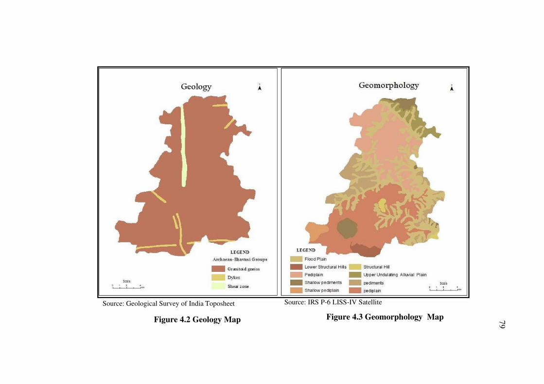
79Figure 4.2 Geology Map Figure 4.3 Geomorphology Map

Source: Geological Survey of India Toposheet Source: IRS P-6 LISS-IV Satellite

80

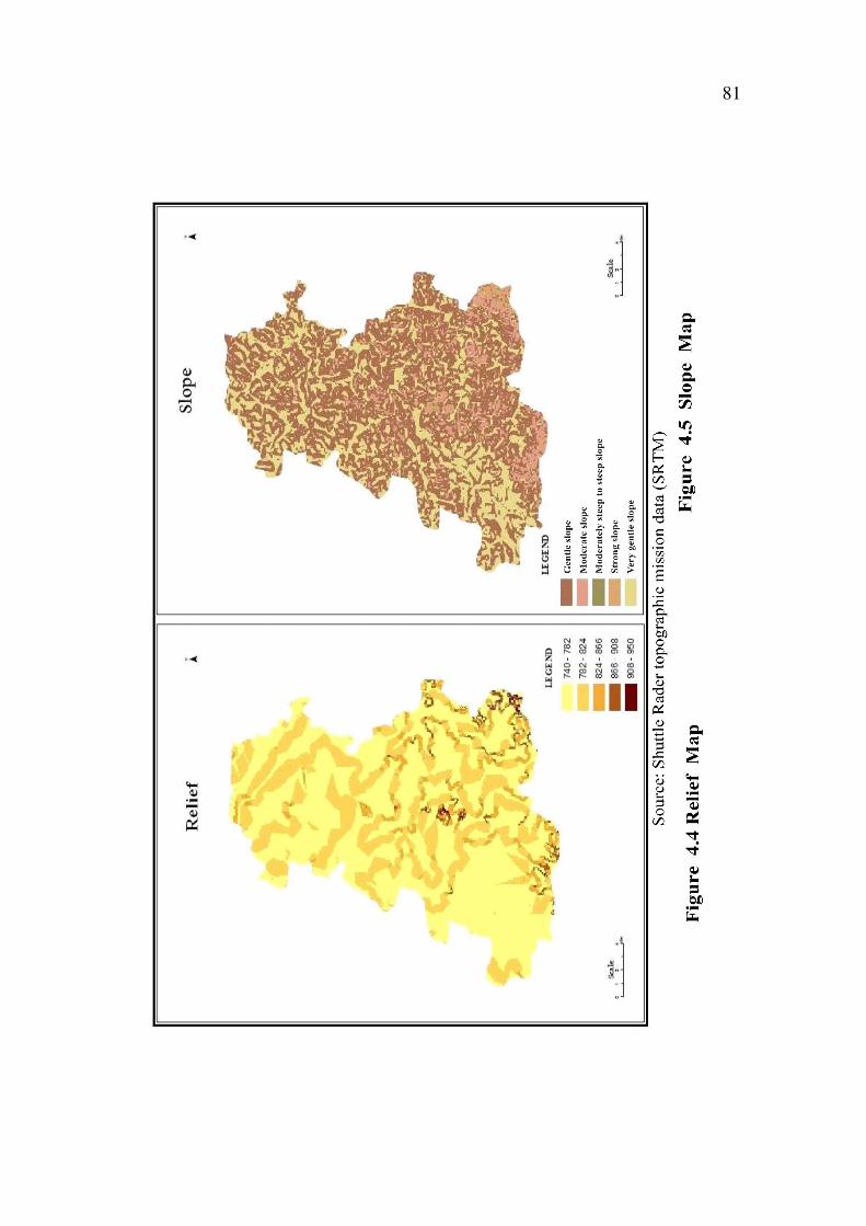
4.2.4 Relief Map

Relief map refer to a three dimensional representation of the terrain

or two dimensional map using cartographic relief depiction to represent the

terrain. A topographical map is a type of map characterized by large scale

detail and quantitative representation of relief, using contour lines in modern

mapping, but historically using variety of ways. A contour line is a

combination of two line segments that connect but do not intersect. They

represent the elevation on a topographic map.

Relief map was analyzed from x, y, z data collected from Shuttle

radar topographic mission data with 90 m resolution (SRTM). Slope map was

prepared from relief map, using Arc GIS 9.1. The Relief map and Slope map

shown in the Figure 4.4 and Figure 4.5. From the map it was observed that,

the central part of the study area houses Chanthirasudesuvararmalai 950 m

above mean sea level and TVS motor company 940 m above the mean sea

level, Bagalur on the northern part 870 m, Soodalam on the south 900 m,

Dinnur on the eastern part 860 m and Zuzuvadi on the western part 880m

above mean sea level.

4.2.4.1 Slope Map

Slope of an area is an indicator of infiltration rate. The places

where the slope is more, contact period of water with surface is less and the

infiltration rate will be less. In places where relatively less, the contact of

water with the surface will be high and the infiltration rate will also be high

which results in good groundwater potential. The study area was classified

into five categories gentle slope, moderate slope, moderate steep to steep

sloping, strongly sloping and very gentle sloping.

82

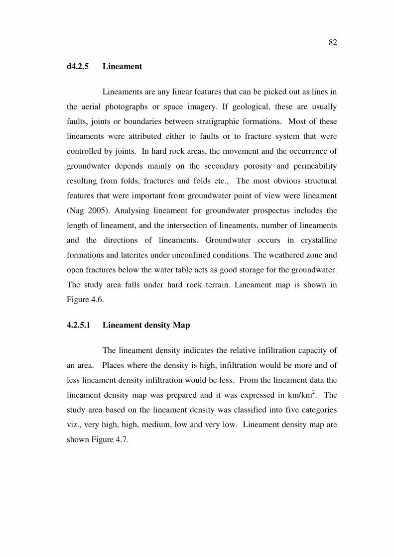
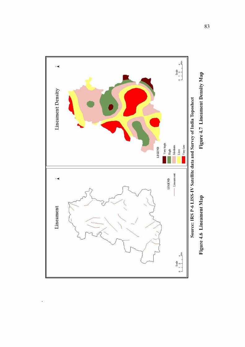
d4.2.5 Lineament

Lineaments are any linear features that can be picked out as lines in

the aerial photographs or space imagery. If geological, these are usually

faults, joints or boundaries between stratigraphic formations. Most of these

lineaments were attributed either to faults or to fracture system that were

controlled by joints. In hard rock areas, the movement and the occurrence of

groundwater depends mainly on the secondary porosity and permeability

resulting from folds, fractures and folds etc., The most obvious structural

features that were important from groundwater point of view were lineament

(Nag 2005). Analysing lineament for groundwater prospectus includes the

length of lineament, and the intersection of lineaments, number of lineaments

and the directions of lineaments. Groundwater occurs in crystalline

formations and laterites under unconfined conditions. The weathered zone and

open fractures below the water table acts as good storage for the groundwater.

The study area falls under hard rock terrain. Lineament map is shown in

Figure 4.6.

4.2.5.1 Lineament density Map

The lineament density indicates the relative infiltration capacity of

an area. Places where the density is high, infiltration would be more and of

less lineament density infiltration would be less. From the lineament data the

lineament density map was prepared and it was expressed in km/km2. The

study area based on the lineament density was classified into five categories

viz., very high, high, medium, low and very low. Lineament density map are

shown Figure 4.7.

84

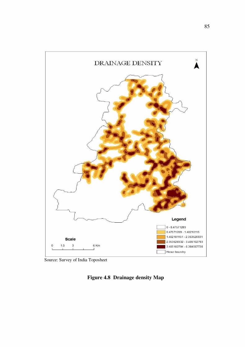
4.2.6 Drainage

The drainage pattern has been one of the most important indicators

of hydrogeological features because drainage, texture and density were

controlled in a fundamental way by the underlying lithology (Charoan 1974).

Drainage map shows us the direction of flow of surface water. Groundwater

in a particular area is based on infiltration of surface water, so the flow

direction of the surface water is important. This could be identified by the

pattern of drainage.

4.2.6.1 Drainage density Map

Drainage density indicates closeness of spacing of channels as well

as the nature of surface material (Prasad et al 2007). It was the measure of the

total length of the stream segment of all orders per unit area expressed in

km/km2. Drainage density was affected by factors which control the

characteristics length of the stream like resistance to weathering, permeability

of rock formation, climate, vegetation etc., (Rajiv Chopra et al 2005). It is an

important criterion particularly with respect to the rock type. Since the

drainage density can indirectly indicate the groundwater prospectus of an area

due to its relation with surface runoff and permeability, the same was

considered as one of the indicators of groundwater occurrence. Drainage

density was classified into different classes varying very low to very high

density. The zones of high drainage density will have poor groundwater

prospectus and gradually the zones of lower and lower drainage density will

have better groundwater prospectus. The drainage density map is shown in the

Figure 4.8.

85

Source: Survey of India Toposheet

Figure 4.8 Drainage density Map

86

4.2.7 Soil Map

Soil is the upper weathered part of the earth’s surface. Soil is

formed due to combined action of rocks, topography and climate and it

comprises of different mineral particles, water, air and humus. Soils of India

are classified based on their colour, structure and place where they are found.

Infiltration capacity of the soil is important for groundwater recharge which

increases the level of groundwater. Interface between the surface and

groundwater is mainly influenced by soil. So to explore groundwater, soil

cover of the study area as to be considered.

The hydrological soil map shown in Figure 4.9 was classified as

clayey, fine loamy and loamy soils. It was observed that the clayey soil cover

an area of 93.14 square kilometre of the total area, fine loamy covers an area

of 172.01 square kilometre which occupies the major share and loamy soil

covers an area 10.14 square kilometre respectively. Fine loamy soils do not

allow the water to percolate into the ground surface are more prominent in the

study area.

87

Source: National Board of Soil Survey (NBSS)

Figure 4.9 Soil Map

88

4.3 STUDY OF RAINFALL CHARACTERISTICS

A systematic analysis of rainfall and its trend will help to

understand the behavior of the rainfall occurrence and would solve many

problems related to the water management. From the rainfall characteristics

study the rainfall is classified into annual and seasonal rainfall. The

classification of annual and seasonal rainfall is shown in Table 4.2.

4.3.1 Annual rainfall Analysis

From the Table, it was observed that the average values of annual

and monsoon rainfall were 810 mm and 567 mm respectively. The standard

deviation for annual and monsoon rainfall were 386 mm and 314 mm and the

coefficient of variation of 48 percent and 55 percent respectively. The month

of September received maximum rainfall of 495 mm in the year 2005,

followed by rainfall of 453 mm in the month of October in the year 1999.

The month of January was found to be the driest month with an average

rainfall of 2.16 mm. During the study period of 19 years, 77 percent was

observed as normal rainfall, 5 percent as drought and 18 percent as excess

rainfall. It was also observed that in the monsoon period about 88 percent

rainfall was normal, 5 percent drought and 7 percent in excess. The highest

and lowest rainfall was 1805 mm and 286 mm occurred in the year 2008 and

1990 respectively. The drought year was noticed in the year 1990. From the

above discussion it is observed that the area receives more rainfall during

monsoon season, which can be conserved by various artificial recharge

structures in order to effectively use the water throughout the year.

89

Table 4.2 Classification of Annual and Seasonal rainfall

Rainfall (mm) Classification

Year Annual Monsoon Annual Monsoon

1990 286 196.6 Drought Drought

1991 877.6 573.5 Normal Normal


1993 576.59 349.99 Normal Normal






1999 1190.2 869.2 Normal Normal

2000 1198.1 909.7 Excess Excess




2004 1152.4 668 Normal Normal

2005 1368 1022 Excess Excess

2006 552 331.1 Excess Normal

2007 972 667 Normal Normal

2008 1805.8 1477.8 Excess Excess

Mean 810.49 567.15 14 Normal 16 Normal

Std. Dev. 386.94 314.27 4 Excess 2 Excess

Coefficient of

variation

47.74 55.41 1 Drought 1 Drought

90

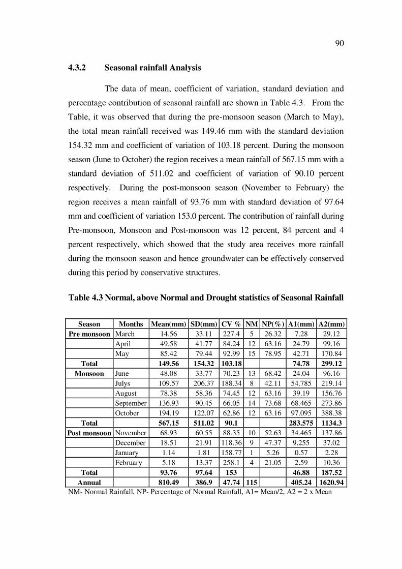
4.3.2 Seasonal rainfall Analysis

The data of mean, coefficient of variation, standard deviation and

percentage contribution of seasonal rainfall are shown in Table 4.3. From the

Table, it was observed that during the pre-monsoon season (March to May),

the total mean rainfall received was 149.46 mm with the standard deviation

154.32 mm and coefficient of variation of 103.18 percent. During the monsoon

season (June to October) the region receives a mean rainfall of 567.15 mm with a

standard deviation of 511.02 and coefficient of variation of 90.10 percent

respectively. During the post-monsoon season (November to February) the

region receives a mean rainfall of 93.76 mm with standard deviation of 97.64

mm and coefficient of variation 153.0 percent. The contribution of rainfall during

Pre-monsoon, Monsoon and Post-monsoon was 12 percent, 84 percent and 4

percent respectively, which showed that the study area receives more rainfall

during the monsoon season and hence groundwater can be effectively conserved

during this period by conservative structures.

Table 4.3 Normal, above Normal and Drought statistics of Seasonal Rainfall

Season Months Mean(mm) SD(mm) CV % NM NP(%) A1(mm) A2(mm)

Pre monsoon March 14.56 33.11 227.4 5 26.32 7.28 29.12

April 49.58 41.77 84.24 12 63.16 24.79 99.16

May 85.42 79.44 92.99 15 78.95 42.71 170.84

Total 149.56 154.32 103.18 74.78 299.12

Monsoon June 48.08 33.77 70.23 13 68.42 24.04 96.16

Julys 109.57 206.37 188.34 8 42.11 54.785 219.14

August 78.38 58.36 74.45 12 63.16 39.19 156.76

September 136.93 90.45 66.05 14 73.68 68.465 273.86

October 194.19 122.07 62.86 12 63.16 97.095 388.38

Total 567.15 511.02 90.1 283.575 1134.3

Post monsoon November 68.93 60.55 88.35 10 52.63 34.465 137.86

December 18.51 21.91 118.36 9 47.37 9.255 37.02

January 1.14 1.81 158.77 1 5.26 0.57 2.28

February 5.18 13.37 258.1 4 21.05 2.59 10.36

Total 93.76 97.64 153 46.88 187.52

Annual 810.49 386.9 47.74 115 405.24 1620.94

NM- Normal Rainfall, NP- Percentage of Normal Rainfall, A1= Mean/2, A2 = 2 x Mean

91

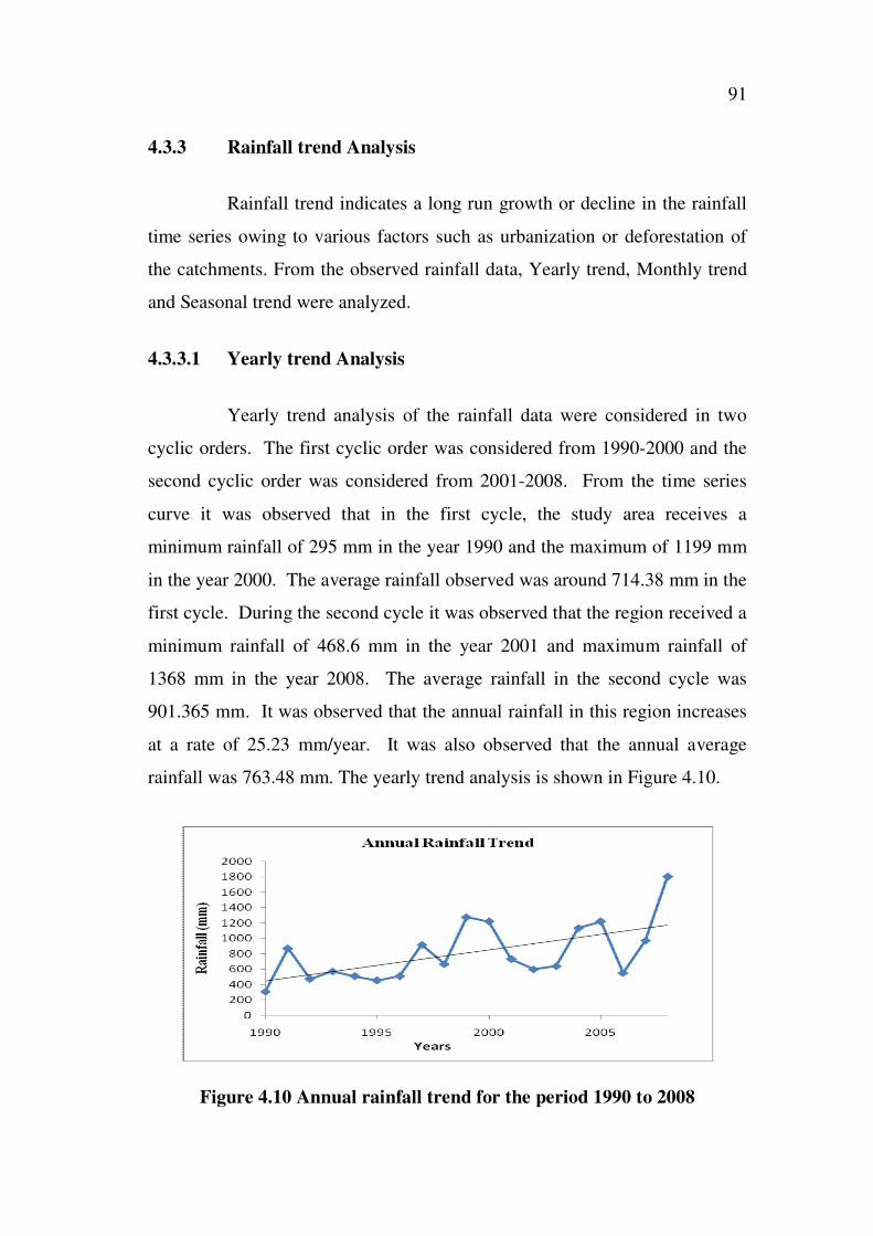
4.3.3 Rainfall trend Analysis

Rainfall trend indicates a long run growth or decline in the rainfall

time series owing to various factors such as urbanization or deforestation of

the catchments. From the observed rainfall data, Yearly trend, Monthly trend

and Seasonal trend were analyzed.

4.3.3.1 Yearly trend Analysis

Yearly trend analysis of the rainfall data were considered in two

cyclic orders. The first cyclic order was considered from 1990-2000 and the

second cyclic order was considered from 2001-2008. From the time series

curve it was observed that in the first cycle, the study area receives a

minimum rainfall of 295 mm in the year 1990 and the maximum of 1199 mm

in the year 2000. The average rainfall observed was around 714.38 mm in the

first cycle. During the second cycle it was observed that the region received a

minimum rainfall of 468.6 mm in the year 2001 and maximum rainfall of

1368 mm in the year 2008. The average rainfall in the second cycle was

901.365 mm. It was observed that the annual rainfall in this region increases

at a rate of 25.23 mm/year. It was also observed that the annual average

rainfall was 763.48 mm. The yearly trend analysis is shown in Figure 4.10.

Figure 4.10 Annual rainfall trend for the period 1990 to 2008

92

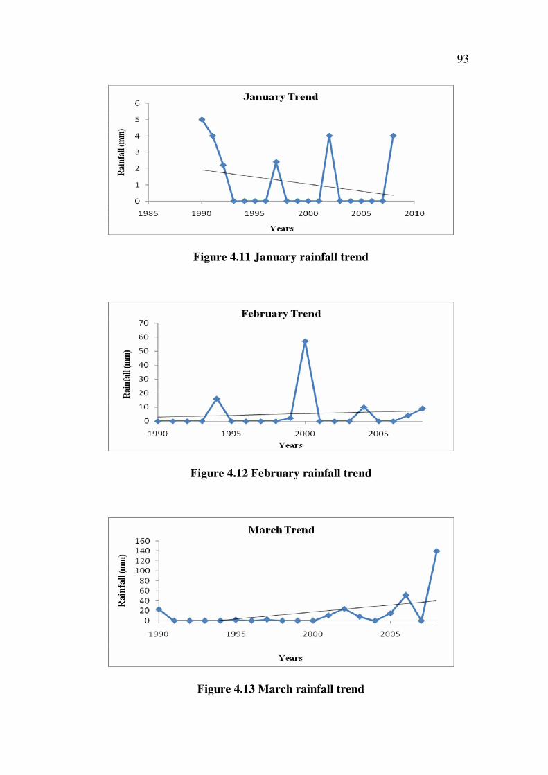
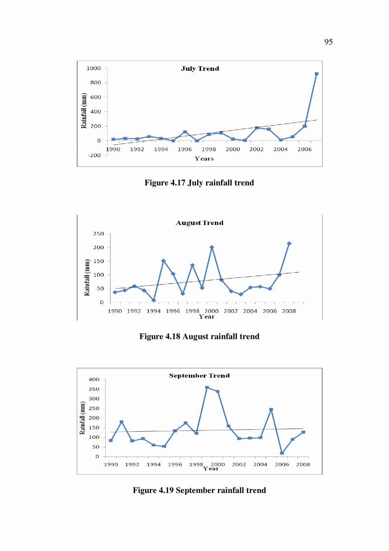
4.3.3.2 Monthly trend Analysis

The monthly trend analysis are shown in Figure 4.11 to

Figure 4.22. From the monthly trend graph, it was observed that during the

month of January, February, March and December there was very little rain or

no rain at all. In the month of April and May due to pre-monsoon showers, it

was observed that the moving average shows an increasing trend and is more

pronounced in the recent years. Rainfall during the month of June, July and

August decrease at a rate of 3.14 mm, 6.35 mm and 9.99 mm/month. During

the month of October the trend analysis shows that there is increasing trend of

about 13 mm/month. The rainfall in the month of November also showed a

slight increase at a rate of 0.566 mm/month.

4.3.3.3 Seasonal trend Analysis (Premonsoon, Monsoon, Post monsoon)

Season wise trend analysis are shown in Figure 4.23 to Figure 4.25.

From the analysis it was observed that the average rainfall in the Pre-monsoon

season (March to May) was 49.85 mm and highest and the lowest rainfall was

85.42 mm and 14.56 mm respectively. It was observed that the rainfall

increases at a rate of 23.95 mm /season. It also indicates that rainfall was

above the moving average for the period of seven years and for the remaining

period the rainfall was below the moving average line.

During the Monsoon season the trend analysis showed that the

average rainfall received was 43.43 mm and is highest and lowest rainfall

received was 194.19 mm and 68.93 mm respectively. From the trend line it

was observed that the rainfall was above the moving average for a period of

six years and below for the rest of the years. During the Post monsoon season

the trend analysis shows that the average rainfall received was 27.14 mm and

its highest and lowest rainfall received was 68.93 mm and 1.14 mm

respectively. From the trend line it was observed that the rainfall was above

the moving average for a period of ten years and below for the rest of the

years.

93

Figure 4.11 January rainfall trend

Figure 4.12 February rainfall trend

Figure 4.13 March rainfall trend

94

Figure 4.14 April rainfall trend

Figure 4.15 May rainfall trend

Figure 4.16 June rainfall trend

95

Figure 4.17 July rainfall trend

Figure 4.18 August rainfall trend

Figure 4.19 September rainfall trend

96

Figure 4.20 October rainfall trend

Figure 4.21 November rainfall trend

Figure 4.22 December rainfall trend

97

Figure 4.23 Pre monsoon rainfall trend

Figure 4.24 Monsoon rainfall trend

Figure 4.25 Post monsoon rainfall trend

98

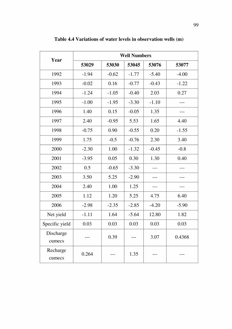
4.4 ASSESSMENT OF GROUNDWATER POTENTIAL

Assessment of groundwater potential was calculated by water table

fluctuation method recommended by groundwater estimation committee

(GEC 1997). The variations of water level fluctuations are shown in Table

4.4. Based on the analysis it was observed that the quantity of water pumped

out in the aquifer was 3.89 million cubic metre /year and the recharge rate

was estimated as 1.614 million cubic metre /year. Hence, it indicates that in

the study area as a whole, the groundwater discharge rate was more than the

recharge, which leads to groundwater depletion. The estimated safe

groundwater potential was 36.5 million cubic metre and the net safe yield

after subtracting the overdraft and evaporation loss was 31.025 million cubic

metre.

From the field data, the variations of water level fluctuations with

the amount of rainfall in each observation wells are shown in Figure 4.26 to

Figure 4.30. The results showed that there was a gradual rise in the water

level with the increase in rainfall from the year 1992-2003. However, there

was a decrease in water level in most of the observation wells even though an

increase in rainfall from the year 2004 to 2006. The net results of the study

clearly indicate that there was depletion in the groundwater potential. This is

mainly due to an unexpected demographic explosion, industrialization and

urbanization.

99

Table 4.4 Variations of water levels in observation wells (m)

Well NumbersYear

53029 53030 53045 53076 53077

1992 -1.94 -0.62 -1.77 -5.40 -4.00

1993 -0.02 0.16 -0.77 -0.43 -1.22

1994 -1.24 -1.05 -0.40 2.03 0.27

1995 -1.00 -1.95 -3.30 -1.10 ---

1996 1.40 0.15 -0.05 1.35 ---

1997 2.40 -0.95 5.53 1.65 4.40

1998 -0.75 0.90 -0.55 0.20 -1.55

1999 1.75 -0.5 -0.76 2.30 3.40

2000 -2.30 1.00 -1.32 -0.45 -0.8

2001 -3.95 0.05 0.30 1.30 0.40

2002 0.5 -0.65 -3.30 --- ---

2003 3.50 5.25 -2.90 --- ---

2004 2.40 1.00 1.25 --- ---

2005 1.12 1.20 5.25 4.75 6.40

2006 -2.98 -2.35 -2.85 -4.20 -5.90

Net yield -1.11 1.64 -5.64 12.80 1.82

Specific yield 0.03 0.03 0.03 0.03 0.03

Discharge

cumecs--- 0.39 --- 3.07 0.4368

Recharge

cumecs0.264 --- 1.35 --- ---

100

Figure 4.26 Variation of water level in well No.53029



801

802

803

804

805

806

807

808

0

200

400

600

800

1000

1992

1993

1994

1995

1996

1997

1998

1999

2000

2001

2002

2003

2004

Wate

r le

ve

l flu

ctati

on

(m

)

Rain

fall

(m

m)

Year

rainfall

depth

101

0

200

400

600

800

1000

1992

1993

1994

1995

1996

1997

1998

1999

2000

2001

2002

2003

2004

2005

2006

Year

Rain

fall

(m

m)

812

814

816

818

820

822

824

Wate

r L

evel

Flu

ctu

ati

on

(m

)



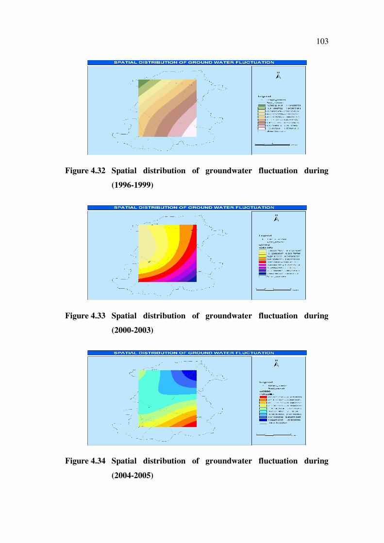
4.4.1 Analysis of groundwater level fluctuation using GIS

The groundwater fluctuations in and around the study area with

varying rainfall were analyzed using GIS. Spatial interpolation technique was

used for the analysis. The continuous surfaces of groundwater levels for every

four year interval were shown in Figure 4.31 to Figure 4.35. From the figure,

it can be observed that during the year 1992, the southern part of the study

area like Hosur town, Sipcot region has water level varying from 0.6 m to -

0.4 m below the reference water table. Even though this region received a

good amount of rainfall of about 495 mm in the same year, but it showed poor

0

200

400

600

800

1000

1992

1993

1994

1995

1996

1997

1998

1999

2000

2001

2002

2003

2004

2005

2006

Year

Rain

fall

(m

m)

812

814

816

818

820

822

824

Wate

r L

evel

Flu

ctu

ati

on

(m

)

102

groundwater potential in this region. This is mainly due to overexploitation

of groundwater in the region due to Industrialization and urbanization.

However, the northern part of the study area comprising of villages like

Kagganur, Sevaganapalli showed that the variation in the water wells ranging

from 3 m to 7 m above the groundwater table. This indicates good amount of

Groundwater potential in the region. It was due to the fact that this region

comes under agricultural zone where pumping of water for other purposes

was much less when compared to industrial and urban zones. In the year

1996-2000, overall study area showed low water levels due to failure of

monsoon. This region was also declared as a severe drought prone zone by

Government of Tamil Nadu in the same period. In the year 2004, only a few

regions showed a gradual increase in the groundwater level ranging from 1m

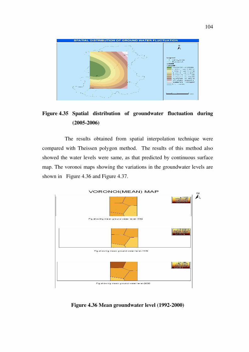
to 2 m above water table. During the year 2006, the overall study area

indicated the negative values ranging from -1 m to - 6 m below water table

even though this region has received highest rainfall of 1368 mm. This was

mainly due to demographic increase in population, urbanization and

industrialization in the region and natural recharge was very low in the region

as it comprises of hard rock terrain.

Figure 4.31 Spatial distribution of groundwater fluctuation during

(1992-1995)

103


(1996-1999)


(2000-2003)


(2004-2005)

104


(2005-2006)

The results obtained from spatial interpolation technique were

compared with Theissen polygon method. The results of this method also

showed the water levels were same, as that predicted by continuous surface

map. The voronoi maps showing the variations in the groundwater levels are

shown in Figure 4.36 and Figure 4.37.

Figure 4.36 Mean groundwater level (1992-2000)

105

Figure 4.37 Mean groundwater level (2001-2004)

4.5 ESTIMATION OF AQUIFER PARAMETER

Aquifer has the ability to store and transmit water. The quantity of

water stored by an aquifer and the water released by it, depends on the nature

and composition of the aquifer which is quantified through certain parameters

like Transmissibility, Permeability and Storage coefficient.

Transmissibility (T) is the discharge through unit depth of the

aquifer for a fully saturated depth under unit hydraulic gradient. It is usually

expressed as lpd/m or m2/sec. It is the product of permeability and saturated

thickness.

Permeability (K) of a material is a measure of its capacity to

transmit water or any other fluid through its interstices. Groundwater is

transmitted through aquifers at a very small velocities ranging from 1 to 500

m/year.

106

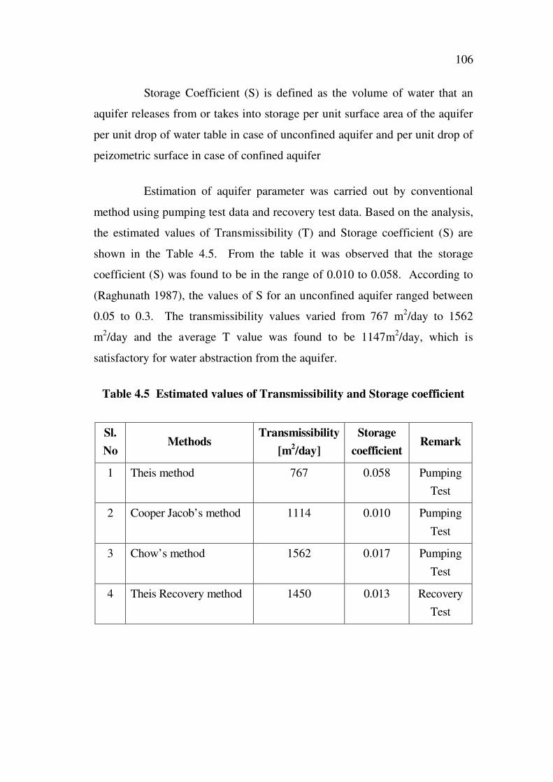
Storage Coefficient (S) is defined as the volume of water that an

aquifer releases from or takes into storage per unit surface area of the aquifer

per unit drop of water table in case of unconfined aquifer and per unit drop of

peizometric surface in case of confined aquifer

Estimation of aquifer parameter was carried out by conventional

method using pumping test data and recovery test data. Based on the analysis,

the estimated values of Transmissibility (T) and Storage coefficient (S) are

shown in the Table 4.5. From the table it was observed that the storage

coefficient (S) was found to be in the range of 0.010 to 0.058. According to

(Raghunath 1987), the values of S for an unconfined aquifer ranged between

0.05 to 0.3. The transmissibility values varied from 767 m2/day to 1562

m2/day and the average T value was found to be 1147m

2/day, which is

satisfactory for water abstraction from the aquifer.

Table 4.5 Estimated values of Transmissibility and Storage coefficient

Sl.

NoMethods

Transmissibility

[m2/day]

Storage

coefficientRemark

1 Theis method 767 0.058 Pumping

Test

2 Cooper Jacob’s method 1114 0.010 Pumping

Test

3 Chow’s method 1562 0.017 Pumping

Test

4 Theis Recovery method 1450 0.013 Recovery

Test

107

4.6 WATER BALANCING STUDY

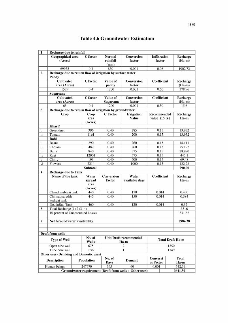
Based on the analysis of the groundwater balancing study it was

observed that net groundwater availability was 2984.38 ha-m or 29.84 million

cubic metre and the groundwater requirement was 3641.39 ha-m or

36.41million cubic metre, which shows a deficit of 6.57 million cubic metre.

The net groundwater availability for the study area is shown in Table 4.6.

4.6.1 Categorization of groundwater development in the study area

Stage of groundwater development = C/B x 100

= (3641.39 / 2984.38) x 100

= 122.01 percent

From the above result it was observed that the value of stage of

groundwater development for the study area can be characterized as

“OVEREXPLOITED” region has its value is greater than 100 percent.

108

Table 4.6 Groundwater Estimation

1 Recharge due to rainfall

Geographical area

(Acres)

C factor Normal

rainfall

(mm)

Conversion

factor

Infiltration

factor

Recharge

(Ha-m)

69953 0.4 850 0.001 0.08 1902.72

2 Recharge due to return flow of irrigation by surface water

Paddy

Cultivated

area (Acres)

C factor Value of

paddy

Conversion

factor

Coefficient Recharge

(Ha-m)

1579 0.4 1200 0.001 0.50 378.96

Sugarcane

Cultivated

area (Acres)

C factor Value of

Sugarcane

Conversion

factor


(Ha-m)

65 0.4 1200 0.001 0.50 15.6

3 Recharge due to return flow of irrigation by groundwater

Crop Crop

area

(Acres)

C factor Irrigation

Value

Recommended

value (15 %)

Recharge

Ha-m

Kharif

i Groundnut 396 0.40 285 0.15 13.932

ii Tomato 1161 0.40 200 0.15 13.932

Rabi

i Beans 290 0.40 260 0.15 18.111

ii Cholam 482 0.40 260 0.15 75.192

iii Bajra 840 0.40 575 0.15 28.980

iv Ragi 12901 0.40 575 0.15 445.1

v Chilly 193 0.40 600 0.15 69.48

vi Flowers 2214 0.40 1000 0.15 132.28

Subtotal 790.00

4 Recharge due to Tank

Name of the tank Water

spread

area

(Acres)

Conversion

factor

Water

available days


Ha-m

Chandrambigai tank 440 0.40 170 0.014 0.430

Chinnappareddykodigai tank

445 0.40 150 0.014 0.384

DoddaRao Tank 460 0.40 120 0.014 0.32

5 Total Recharge (1+2+3+4) 3316

10 percent of Unaccounted Losses 331.62

7 Net Groundwater availability 2984.38

Draft from wells

Type of WellNo. of

Wells

Unit Draft recommended

Ha-mTotal Draft Ha-m

Open tube well 675 2 1350

Tube bore well 1749 1 1749

Other uses (Drinking and Domestic uses)

Description PopulationNo. of

DaysDemand

Conversi

on factor

Total

Ha-m

Human beings 247670 365 60 0.001 542.39

Groundwater requirement (Draft from wells + Other uses) 3641.39

109

4.7 GROUNDWATER QUALITY ANALYSIS

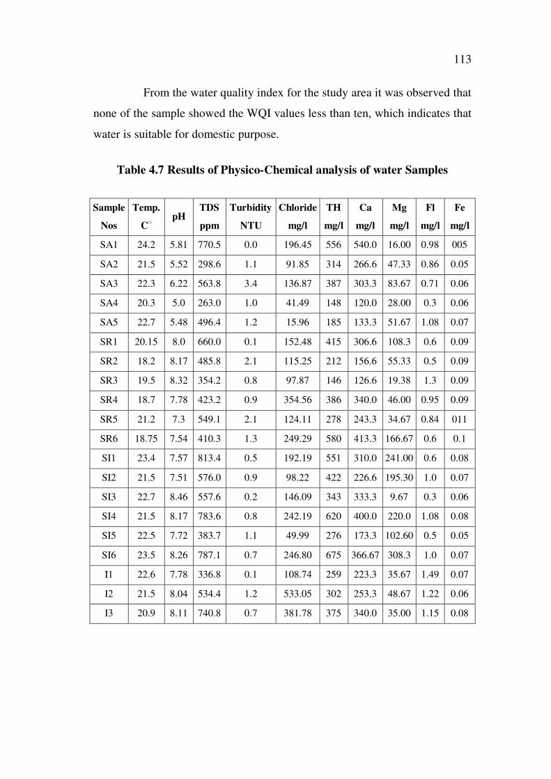
Groundwater quality analysis was carried out for twenty

groundwater samples collected from agricultural, residential, industrial and

institutional zones. The groundwater parameters analyzed were pH, Turbidity,

Total dissolved solids, Chloride, Total hardness, Calcium, Magnesium, Iron

and Fluoride. The results of Physico-chemical parameters of the groundwater

samples are shown in Table 4.7 and the variation of the parameters in the

different zones are shown in Figure 4.38 to Figure 4.45. All the results were

compared with the standard permissible limits as recommended by WHO,

IS-10500-91, ICMR standards. The standards for drinking water shown in

Table 3.5 in chapter 3.

4.7.1 pH

pH indicates the nature of water samples whether it is acidic or

alkaline in nature. Normally water will have pH values ranging from 4 to 9.

pH value of the samples ranges from 7.3 to 8.5 and were within the

permissible limit for most of the samples, except in the agricultural zone

which ranges from 5.0 to 6.33 indicating it is slightly acidic in nature.

4.7.2 Turbidity

Turbidity is the total suspended matter in the water. It is caused by

the presence of insoluble sediments, organisium and organic matter

(Karanth, 1987). Turbidity of the samples varies from 0.5 to 3.4 and were

within the permissible limits.

4.7.3 Total Dissolved Solids (TDS)

Total dissolved solids are the sum of total cations and anions. It

includes the total ionic species such as sodium, potassium, calcium,

magnesium, chloride, bicarbonate, nitrate, sulphate and other trace elements

110

(Mondal et al 2005). It is a measure of the water to carry electric current.

Total dissolved solids of water samples ranges from 263 mg/l to 813.4 mg/l

which shows that most of the samples were within the permissible limits

except SA4, SR2, SR3, SR6 and I1.

4.7.4 Chloride

Chloride is a widely distributed element in all types of rocks in one

or other forms. Its affinity towards sodium is high. Therefore its concentration

is high in groundwater, where temperature is high and rainfall is less. Soil

porosity and permeability also has a key role in building up the chloride

concentration (Chadha 1999). Chloride in water sample ranges from 15.90

mg/l to 533.02 mg/l, which indicates that most of the samples were within the

permissible limits except SR4, I2 and I3.

4.7.5 Total Hardness

Water hardness is caused primarily by the presence of cations such

as calcium and magnesium and anions such as carbonates and bicarbonates,

chloride and sulphate in water (Anbazhgan and Archana Nair 2004). Total

hardness values vary from 148 mg/l to 675 mg/l, which shows that majority of

the samples fall under the hard category.

4.7.6 Calcium

The range of calcium content in groundwater is largely dependent

on calcium carbonate, sulphate and rarely chloride. The solubility of calcium

carbonate varies widely with partial pressure of carbon dioxide in the air in

contact with water (Karanth 1987). Calcium values ranges from 120 mg/l to

413.3 mg/l. which shows that most of the samples exceed the permissible

limits.

111

4.7.7 Magnesium

Magnesium in the water sample ranges from 16 mg/l to 220 mg/l.

indicating most of the samples are exceeding the permissible limits.

4.7.8 Fluoride

Fluoride commonly occurs from fluorine which has a unique

property that if it is in optimum dosage in drinking water it is good for health.

Fluoride level between 1mg/l to 1,5 mg/l gives good resistance for teeth.

Fluoride level above permissible limits leads to staining of the teeth. Fluoride

values for the water samples ranges from 0.3 mg/l to 1.49 mg/l indicating the

values of all the samples were with the permissible limits.

4.7.9 Iron

Iron is present in groundwater due to the dissolution of rocks rich in

iron oxide and the contact of groundwater with metallic pipes which are used

for extracting groundwater. The concentration of iron varies from 0.05 to 0.1

indicating the values of all the samples are within the permissible limits.

The Physico-chemical analysis of the groundwater samples shows

that most of the samples are within the permissible limits and hence it can be

concluded that the available groundwater is suitable for domestic purposes.

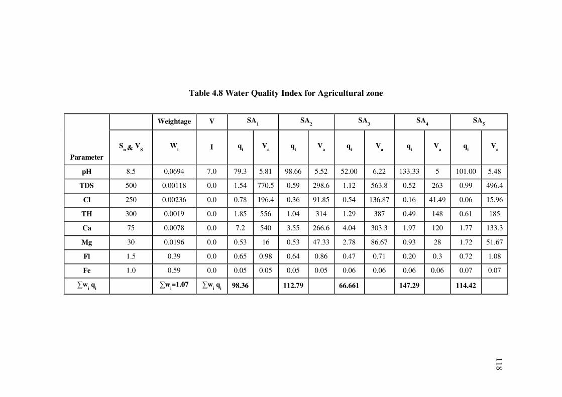
4.8 WATER QUALITY INDEX FOR THE STUDY AREA

Water quality Index (WQI) relates a group of water quality

parameters to a common scale and combines them into a single number in

accordance with the chosen method of computation (Chaturvedi et al 2008). It

is a very useful tool for communicating the information on overall quality of

water (Pradhan et al 2001).

112

Water quality index for the study area for all the samples in various

zones were analyzed by considering decreasing scale indices. Water quality

status based on the WQI is shown in Table 3.7 and Table 3.8 in chapter 3.

Water quality index for all the samples are shown in Table 4.8 to 4.11

respectively. Specimen calculation for the water quality index is shown in

Appendix 2.

Table 4.8 reveals that the water quality index in agricultural zone

varies from 66.67 to 147.29. The minimum value of water quality index was

observed in Poonapalli village and the maximum at Bagalur village which

shows that water quality in Poonapalli village was good and excellent at

Bagalur village.

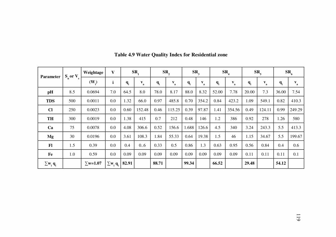
Table 4.9 reveals that water quality index in residential zone varies

from 29.48 to 99.34. The minimum value was observed at Gowri Shankar

Hotel and the maximum value at ASTC Housing board, indicating that the

water quality in and around Gowri Shankar Hotel was very poor and excellent

at ASTC Housing board.

Table 4.10 reveals that water quality index in the Industrial zone

varies from 50.47 to 105.41 showing the minimum value at Ashok Leyland

Phase-I and the maximum value near the Small scale industry at Sipcot-II

which shows that, the water quality in Ashok Leyland Phase-I was poor and

excellent at Sipcot-II.

Table 4.11 reveals that water quality index in the institutional zone

varies from 40.94 to 90.47 having the minimum value of water quality at

Adhiyamaan Educational and Research Institutions (AERI) and the maximum

at Maharishi Higher Secondary School, indicating that the water quality at

AERI Campus was poor and excellent at Maharishi Higher Secondary School,

Hosur.

113

From the water quality index for the study area it was observed that

none of the sample showed the WQI values less than ten, which indicates that

water is suitable for domestic purpose.

Table 4.7 Results of Physico-Chemical analysis of water Samples

Sample

Nos

Temp.

CpH

TDS

ppm

Turbidity

NTU

Chloride

mg/l

TH

mg/l

Ca

mg/l

Mg

mg/l

Fl

mg/l

Fe

mg/l

SA1 24.2 5.81 770.5 0.0 196.45 556 540.0 16.00 0.98 005

SA2 21.5 5.52 298.6 1.1 91.85 314 266.6 47.33 0.86 0.05

SA3 22.3 6.22 563.8 3.4 136.87 387 303.3 83.67 0.71 0.06

SA4 20.3 5.0 263.0 1.0 41.49 148 120.0 28.00 0.3 0.06

SA5 22.7 5.48 496.4 1.2 15.96 185 133.3 51.67 1.08 0.07

SR1 20.15 8.0 660.0 0.1 152.48 415 306.6 108.3 0.6 0.09

SR2 18.2 8.17 485.8 2.1 115.25 212 156.6 55.33 0.5 0.09

SR3 19.5 8.32 354.2 0.8 97.87 146 126.6 19.38 1.3 0.09

SR4 18.7 7.78 423.2 0.9 354.56 386 340.0 46.00 0.95 0.09

SR5 21.2 7.3 549.1 2.1 124.11 278 243.3 34.67 0.84 011

SR6 18.75 7.54 410.3 1.3 249.29 580 413.3 166.67 0.6 0.1

SI1 23.4 7.57 813.4 0.5 192.19 551 310.0 241.00 0.6 0.08

SI2 21.5 7.51 576.0 0.9 98.22 422 226.6 195.30 1.0 0.07

SI3 22.7 8.46 557.6 0.2 146.09 343 333.3 9.67 0.3 0.06

SI4 21.5 8.17 783.6 0.8 242.19 620 400.0 220.0 1.08 0.08

SI5 22.5 7.72 383.7 1.1 49.99 276 173.3 102.60 0.5 0.05

SI6 23.5 8.26 787.1 0.7 246.80 675 366.67 308.3 1.0 0.07

I1 22.6 7.78 336.8 0.1 108.74 259 223.3 35.67 1.49 0.07

I2 21.5 8.04 534.4 1.2 533.05 302 253.3 48.67 1.22 0.06

I3 20.9 8.11 740.8 0.7 381.78 375 340.0 35.00 1.15 0.08

114

Figure 4.38 Variation of pH in Agricultural zone

Figure 4.39 Variation of pH in Residential zone

115

Figure 4.40 Variation of pH in Industrial zone

Figure 4.41 Variation of pH in Institutional zone

116

0

100

200

300

400

500

600

700

800

900

TDS Cl TH Ca Mg Fl Fe

SA1

SA2

SA3

SA4

SA5

Figure 4.42 Variation of Physico chemical parameters in Agricultural

zone

0

100

200

300

400

500

600

700


SR1

SR2

SR3

SR4

SR5

SR6

Figure 4.43 Variation of Physico chemical parameters in Residential zone

117

0

100

200

300

400

500

600

700

800

900


S11

S12

S13

S14

S15

S16

Figure 4.44 Variation of Physico Chemical parameters in Industrail zone

0

100

200

300

400

500

600

700

800


I1

I2

I3

Figure 4.45 Variation of Physico Chemical parameters in Institutional

zone

118

Table 4.8 Water Quality Index for Agricultural zone

Weightage V SA1

SA2

SA3

SA4

SA5

Parameter

Sn & V

SW

i I qi

Va

qi

Va

qi

Va

qi

Va

qi

Va

pH 8.5 0.0694 7.0 79.3 5.81 98.66 5.52 52.00 6.22 133.33 5 101.00 5.48

TDS 500 0.00118 0.0 1.54 770.5 0.59 298.6 1.12 563.8 0.52 263 0.99 496.4

Cl 250 0.00236 0.0 0.78 196.4 0.36 91.85 0.54 136.87 0.16 41.49 0.06 15.96

TH 300 0.0019 0.0 1.85 556 1.04 314 1.29 387 0.49 148 0.61 185

Ca 75 0.0078 0.0 7.2 540 3.55 266.6 4.04 303.3 1.97 120 1.77 133.3

Mg 30 0.0196 0.0 0.53 16 0.53 47.33 2.78 86.67 0.93 28 1.72 51.67

Fl 1.5 0.39 0.0 0.65 0.98 0.64 0.86 0.47 0.71 0.20 0.3 0.72 1.08

Fe 1.0 0.59 0.0 0.05 0.05 0.05 0.05 0.06 0.06 0.06 0.06 0.07 0.07

wi q

iw

i=1.07 w

i q

i 98.36 112.79 66.661 147.29 114.42

119

Table 4.9 Water Quality Index for Residential zone

Weightage V SR1

SR2

SR3

SR4

SR5

SR6

Parameter Snor V

s

(Wi) i q

iv

aq

iv

aq

iv

aq

iv

aq

iv

aq

iv

a

pH 8.5 0.0694 7.0 64.5 8.0 78.0 8.17 88.0 8.32 52.00 7.78 20.00 7.3 36.00 7.54

TDS 500 0.0011 0.0 1.32 66.0 0.97 485.8 0.70 354.2 0.84 423.2 1.09 549.1 0.82 410.3

Cl 250 0.0023 0.0 0.60 152.48 0.46 115.25 0.39 97.87 1.41 354.56 0.49 124.11 0.99 249.29

TH 300 0.0019 0.0 1.38 415 0.7 212 0.48 146 1.2 386 0.92 278 1.26 580

Ca 75 0.0078 0.0 4.08 306.6 0.52 156.6 1.688 126.6 4.5 340 3.24 243.3 5.5 413.3

Mg 30 0.0196 0.0 3.61 108.3 1.84 55.33 0.64 19.38 1.5 46 1.15 34.67 5.5 199.67

Fl 1.5 0.39 0.0 0.4 0..6 0.33 0.5 0.86 1.3 0.63 0.95 0.56 0.84 0.4 0.6

Fe 1.0 0.59 0.0 0.09 0.09 0.09 0.09 0.09 0.09 0.09 0.09 0.11 0.11 0.11 0.1

wi q

iw=1.07 w

i q

i82.91 88.71 99.34 66.52 29.48 54.12

120

Table 4.10 Water Quality Index for Industrial zone

WeightageV SI

1SI

2SI

3SI

4SI

5SI

6

Parameter Sn& V

s

(Wi) i q

iv

aq

iv

aq

iv

aq

iv

aq

iv

aq

iv

a

pH 8.5 0.0694 7 38.0 7.57 34 7.51 97 8.46 78 8.17 48 7.72 84 8.26

TDS 500 0.00118 0.0 1.6 813.4 1.152 576 1.11 557.6 1.56 783.6 0.76 383.7 1.57 787.1

Cl 250 0.00236 0.0 0.76 192.19 0.39 98.22 0.58 146.09 0.96 242.19 0.019 49.99 0.98 246.80

TH 300 0.0019 0.0 1.83 551 0.75 422 1.14 343 2.0 620 0.92 276 2.25 675

Ca 75 0.0078 0.0 4.13 310 3.20 226.6 4.44 333.3 1.16 400 2.31 173.7 4.88 366.67

Mg 30 0.0196 0.0 8.0 241 6.5 19.3 1.28 9.67 7.3 220 3.42 102.6 4.11 308.3

Fl 1.5 0.39 0.0 0.4 0.6 0.66 1.0 0.2 0.3 0.72 1.0 0.33 0.5 0.66 1.0

Fe 1.0 0.59 0.0 0.08 0.08 0.07 0.07 0.06 0.06 0.08 0.08 0.05 0.05 0.07 0.07

wi q

iw

i=1.07 w

i q

i 58.63 50.47 110 98.20 59.70 105.41

121

Table 4.11 Water Quality Index for Institutional zone

I1

I2

I3

ParameterStandard

valuesWeightage v

qi

va

qi

va

qi

va

p H 8.5 0.0694 7.0 31.1 7.78 69.33 8.04 74 8.11

TDS 500 0.00118 0.0 0.67 336.8 1.06 534.4 1.48 740.8

Cl 250 0.00236 0.0 0.43 108.74 2.1 533.05 1.52 381.78

TH 300 0.0019 0.0 0.86 259 1.00 302 1.25 375

Ca 75 0.0078 0.0 2.97 223.3 3.37 253.3 4.5 340

Mg 30 0.0196 0.0 1.18 35.67 1.62 48.67 1.16 32

Fl 1.5 0.39 0.0 0.99 1.46 0.81 1.22 0.766 1.15

Fe 1.0 0.59 0.0 0.07 0.07 0.06 0.06 0.08 0.08

wi q

iw

i=1.07 w

i q

i 40.94 84.90 90.47

122

4.9 SUMMARY

This chapter has focused on the results obtained from the various

analysis carried out. The results from the topographical study indicates that

the percolation of water in the study area was moderate and natural recharge

was low as it is a hard rock terrain. It was observed that the groundwater

levels were depleted due to over exploitation. It is evident from the study that

the more amount of rainfall is received during monsoon season and water can

be effectively stored through conservative structures. It was observed from

the water balancing study that the discharge rate of groundwater was more

than recharge rate and the stage of groundwater development indicated that

the study area falls under overexploited region. Groundwater quality

assessment indicates that available groundwater is suitable for domestic

purposes.

CHAPTER 4 RESULTS AND DISCUSSION -...

Documents

Transcript of CHAPTER 4 RESULTS AND DISCUSSION -...