How does struts work? Mohammad Seyed Alavi [email protected].
Upload
isabel-dayCategory
view
234download
6
2
N-Gram But it must be recognized that the
notion “probability of a sentence” is an entirely useless one, under any known interpretation of this term. Noam Chomsky (1969, p. 57)
Anytime a linguist leaves the group the recognition rate goes up. Fred Jelinek (then of the IBM speech group) (1988)
3
N-grams: Motivation An n-gram is a stretch of text n words long
Approximation of language: information in n-grams tells us something about language, but doesn’t capture the structure
Efficient: finding and using every, e.g., two-word collocation in a text is quick and easy to do
N-grams can help in a variety of NLP applications:
Word prediction = n-grams can be used to aid in predicting the next word of an utterance, based on the previous n- 1 words
Useful for context-sensitive spelling correction, approximation of language, ...
4
Corpus-based NLP Corpus (pl. corpora) = a computer-
readable collection of text and/or speech, often with annotations We can use corpora to gather probabilities
and other information about language us We can say that a corpus used to gather prior
information is training data Testing data, by contrast, is the data one uses to
test the accuracy of a method We can distinguish types and tokens in a
corpus type = distinct word (e.g., like) token = distinct occurrence of a word (e.g., the type
like might have 20,000 tokens in a corpus)
5
Corpora Brown: Brown corpus is a 1 million word
collection of samples from 500 written texts from different genres
Switchboard: corpus of telephone conversations between strangers was collected in the early 1990s and contains 2430 conversations averaging 6 minutes each, totaling 240 hours of speech and about 3 million words

6
Different challenges in corpora Punctuation? Utterance (Uh, Um, …)? Case Sensitive? Inflected word?
Lemma: set of lexical form having same stem, same POS tag, same sense
In rich morphological languages, like Arabic, Persian, need to deal with lemmatization but in English it’s easier to deal with wordforms

7
Simple n-grams Let’s assume we want to predict the next word, based
on the previous context of I dreamed I saw the knights in What we want to find is the likelihood of w8 being the next word, given that we’ve seen w1, ..., w7, in other words,P(w1, ..., w8)
In general, for wn, we are looking for:(1) P(w1, ..., wn) = P(w1)P(w2|w1)...P(wn|w1, ..., wn-1)
But these probabilities are impractical to calculate: they hardly ever occur in a corpus, if at all. (And it would be a lot of data to store, if we could calculate them.)

8
Unigrams So, we can approximate these
probabilities to a particular n-gram, for a given n. What should n be? Unigrams (n= 1):
(2) P(wn|w1, ..., wn-1) ≈ P(wn) Easy to calculate, but we have no contextual
information(3) The quick brown fox jumped
We would like to say that over has a higher probability in this context than lazy does.

9
Bigrams
bigrams (n= 2) are a better choice and still easy to calculate:(4) P(wn|w1, ..., wn-1) ≈ P(wn|wn-1)
(5) P( over| The, quick, brown, fox, jumped) ≈ P( over| jumped)
And thus, we obtain for the probability of a sentence:(6) P(w1, ..., wn) = P(w1)P(w2|w1)P(w3|w2)...P(wn|wn-1)

10
Markov models A bigram model is also called a first-
order Markov model because it has one element of memory (one token in the past) Markov models are the class of probabilistic
models that assume that we can predict the probability of some future unit without looking too far into the past.
Markov models are essentially weighted FSAs—i.e., the arcs between states have probabilities
The states in the FSA are words Much more on Markov models when we hit
POS tagging ...
11
Bigram example What is the probability of seeing the
sentence The quick brown fox jumped over the lazy dog?
(7) P(The quick brown fox jumped over the lazy dog) =P( The| < start >) P( quick| The)P( brown| quick)...P( dog| lazy)
Probabilities are generally small, so log probabilities are usually used
Does this favor shorter sentences?

12
Trigrams
If bigrams are good, then trigrams ( n= 3) can be even better.
Wider context: P( know| did, he) vs. P( know| he)
Generally, trigrams are still short enough that we will have enough data to gather accurate probabilities

13
Training n-gram models Go through corpus and calculate
relative frequencies: (8) P(wn|wn-1) = C(wn-1,wn) / C(wn-1) (9) P(wn|wn-2, wn-1) = C(wn-2,wn-1,wn) / C(wn-2,wn-1)
This technique of gathering probabilities from a training corpus is called maximum likelihood estimation (MLE)

14
Maximum likelihood estimation (MLE) In MLE, the resulting parameter set
maximizes the likelihood of the training set T given the modelM (i.e., P(T|M)).
Example: Chinese occurs 400 times in 1 million words Brown corpus. That is MLE = 0.0004 .
0.0004 is not the best possible estimate of the probability of Chinese occurring in all situation, But it is the probability that makes it most likely that Chinese will occur 400 times in a million-word corpus

15
Know your corpus We mentioned earlier about having
training data and testing data ... it’s important to remember what your training data is when applying your technology to new data If you train your trigram model on
Shakespeare, then you have learned the probabilities in Shakespeare, not the probabilities of English overall
What corpus you use depends on what you want to do later
16
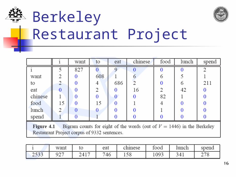
BerkeleyRestaurant Project

17
BerkeleyRestaurant Project

18

19
WSJ trained

20
Open versus closed vocabulary tasks closed vocabulary assumption Unknown word(out of vocabulary)
OOV rate Should to model OOV
Choose a vocabulary (word list) which is fixed in advance.
Convert in the training set any word that is not in this set (any OOV word) to the unknown word token <UNK> in a text normalization step.
Estimate the probabilities for <UNK> from its counts just like any other regular word in the training set.

21
Evaluating N-gram extrinsic evaluation: embed the
model in an application and measure the total performance of the application Very expensive
intrinsitic evaluation metric is one which measures the quality of a model independent of any application Perplexity measure
22
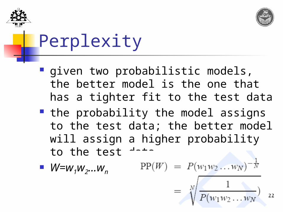
Perplexity given two probabilistic models, the
better model is the one that has a tighter fit to the test data
the probability the model assigns to the test data; the better model will assign a higher probability to the test data
W=w1w2…wn
23
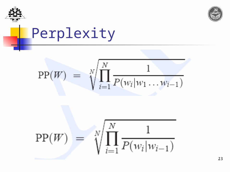
Perplexity
24
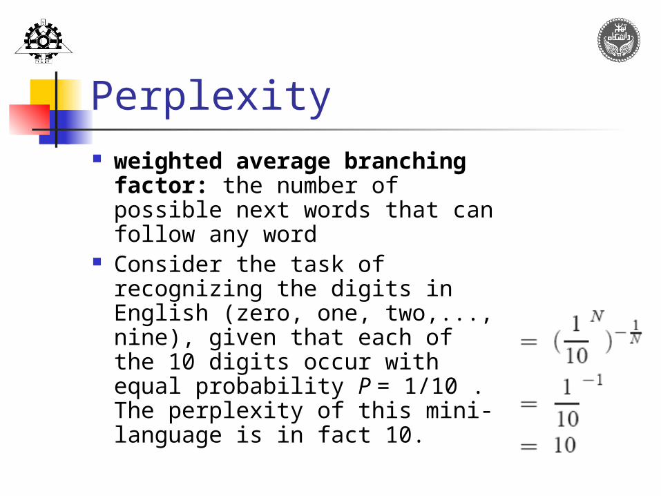
Perplexity weighted average
branching factor: the number of possible next words that can follow any word
Consider the task of recognizing the digits in English (zero, one, two,..., nine), given that each of the 10 digits occur with equal probability P = 1/10 . The perplexity of this mini-language is in fact 10.

25
Perplexity example
WSJ

26
Smoothing: Motivation Let’s assume that we have a good corpus and
have trained a bigram model on it, i.e., learned MLE probabilities for bigrams
But we won’t have seen every possible bigramlickety split is a possible English bigram, but it may not be in the corpus
This is a problem of data sparseness there are zero probability bigrams which are actual possible bigrams in the language
To account for this sparseness, we turn to smoothing techniques making zero probabilities non-zero, i.e., adjusting probabilities to account for unseen data
27
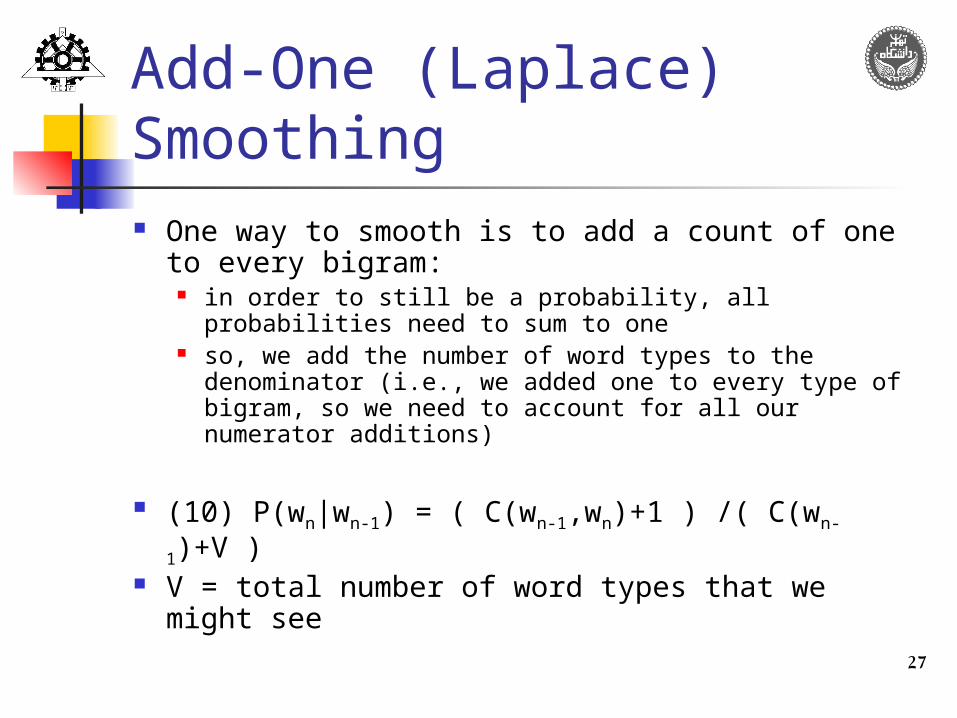
Add-One (Laplace) Smoothing One way to smooth is to add a count of one to
every bigram: in order to still be a probability, all probabilities need
to sum to one so, we add the number of word types to the
denominator (i.e., we added one to every type of bigram, so we need to account for all our numerator additions)
(10) P(wn|wn-1) = ( C(wn-1,wn)+1 ) /( C(wn-1)+V ) V = total number of word types that we might
see

28
Add-One smoothing
P(Wx) = C(Wx) / iC(Wi) Adjusted Count
C*i = (Ci+1)(N/(N+V))
Discount dc = c*/c P*
i = (ci+1)/(N+V) P(Wn|Wn-1)=(C(Wn-1Wn)+1)/(C(Wn-1)+V)

29
Smoothing example So, if treasure trove never occurred in the
data, but treasure occurred twice, we have: (11) P(trove | treasure) = (0+1)/(2+V)
The probability won’t be very high, but it will be better than 0 If all the surrounding probabilities are still high,
then treasure trove could still be the best pick If the probability were zero, there would be no
chance of it appearing.

30
Berkeley Restaurant project

31
C(want to) : 608 to 238 P(to | want) : 0.66 to 0.26 Large changes ! Need to be more accurate …

32
Discounting
An alternate way of viewing smoothing is as discounting Lowering non-zero counts to get the
probability mass we need for the zero count items
The discounting factor can be defined as the ratio of the smoothed count to the MLE count

33
Witten-Bell Discounting Use the count of things you’ve seen once to
help estimate the count of things you’ve never seen
Probability of seeing an N-gram for the first time: counting the number of times we saw N-grams for the first time in the training corpus i:ci=0 pi
* = T/(T+N) The above value is the total probability, should be
divided by total number that is Z=i:ci=0 1 P*
i=T/Z(T+N)

34
Witten-Bell Discounting
Pi* = ci/(N+T) if(ci>0)
ci* = T/Z . N/(N+T) if(ci = 0)
ci* = ci . N/(N+T) if(ci > 0)
35
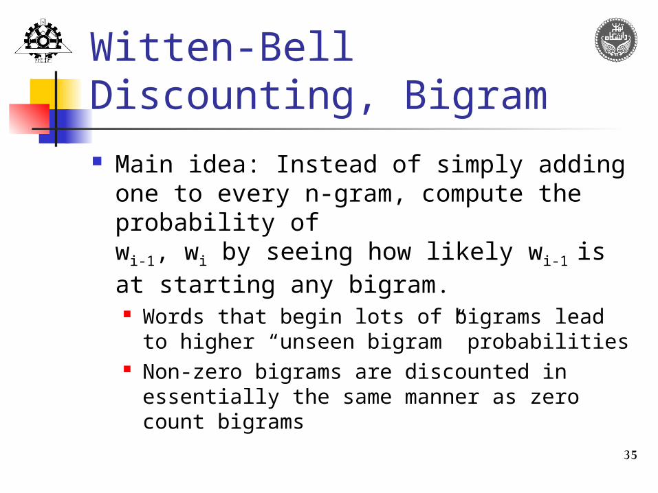
Witten-Bell Discounting, Bigram Main idea: Instead of simply adding one
to every n-gram, compute the probability of wi-1, wi by seeing how likely wi-1 is at starting any bigram. Words that begin lots of bigrams lead to
higher “unseen bigram” probabilities Non-zero bigrams are discounted in
essentially the same manner as zero count bigrams

36
Witten-Bell Discounting formula (12) zero count bigrams:
p*(wi|wi-1) =T(wi-1)/ (Z(wi-1) ( N(wi-1)+T(wi-1)) ) T(wi-1) = the number of bigram types starting with wi-1
N(wi-1) = the number of bigram tokens starting with wi-1
N(wi-1) + T(wi-1) gives us the total number of “events” to divide by
Z(wi-1) = the number of bigram tokens starting with wi-1 and having zero count
this just distributes the probability mass between all zero count bigrams starting with wi-1

37
Good Turing discouting
Using Joint Probability instead of conditional probability i.e. P(wxwi) instead of p(wi|wx)
The main idea is to re-estimate the amount of probability mass to assign to N-grams with zero or low counts by looking at the number of N-grams with higher counts.
38
Good Turing discouting
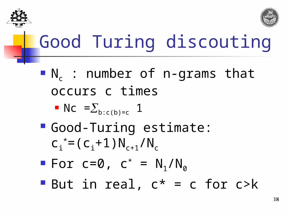
Nc : number of n-grams that occurs c times Nc =b:c(b)=c 1
Good-Turing estimate: ci
*=(ci+1)Nc+1/Nc
For c=0, c* = N1/N0
But in real, c* = c for c>k

39
Example Suppose we are fishing in a lake with 8
species (bass, carp, catfish, eel, perch, salmon, trout, whitefish) and we have seen 6 species with the following counts: 10 carp, 3 perch, 2 whitefish, 1 trout, 1 salmon, and 1 eel (so we haven’t yet seen the catfish or bass)

40
Another example

41
Better estimation Discounting can help to solve the problem of
zero frequency N-grams But it’s not the only knowledge to be used If the tri-gram probability is zero use bi-gram
probability If the bi-gram probability is zero use uni-gram
probability Backoff Interpolation

42
Backoff models: Basic idea Let’s say we’re using a trigram
model for predicting language, and we haven’t seen a particular trigram before. But maybe we’ve seen the bigram, or
if not, the unigram information would be useful
Backoff models allow one to try the most informative n-gram first and then back off to lower n-grams
43
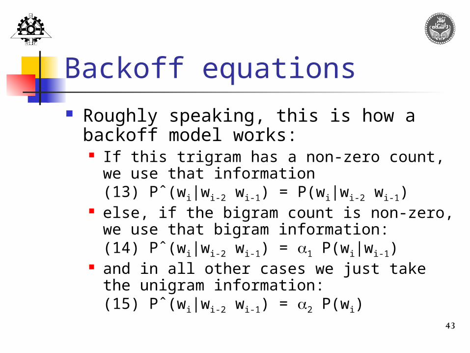
Backoff equations Roughly speaking, this is how a backoff
model works: If this trigram has a non-zero count, we use
that information(13) Pˆ(wi|wi-2 wi-1) = P(wi|wi-2 wi-1)
else, if the bigram count is non-zero, we use that bigram information:(14) Pˆ(wi|wi-2 wi-1) = 1 P(wi|wi-1)
and in all other cases we just take the unigram information:(15) Pˆ(wi|wi-2 wi-1) = 2 P(wi)

44
Backoff models: example Let’s say we’ve never seen the trigram
“maples want more” before But we have seen “want more”, so we can use
that bigram to calculate a probability estimate. So, we look at P(more|want) ... But we’re now assigning probability to
P(more|maples, want) which was zero before we won’t have a true probability model anymore
This is why 1 was used in the previous equations, to assign less re-weight to the probability.
In general, backoff models have to be combined with discounting models

45
Deleted (simple) Interpolation
Deleted interpolation is similar to backing off, except that we always use the bigram and unigram information to calculate the probability estimate
Every trigram probability, then, is a composite of the focus word’s trigram, bigram, and unigram.
46
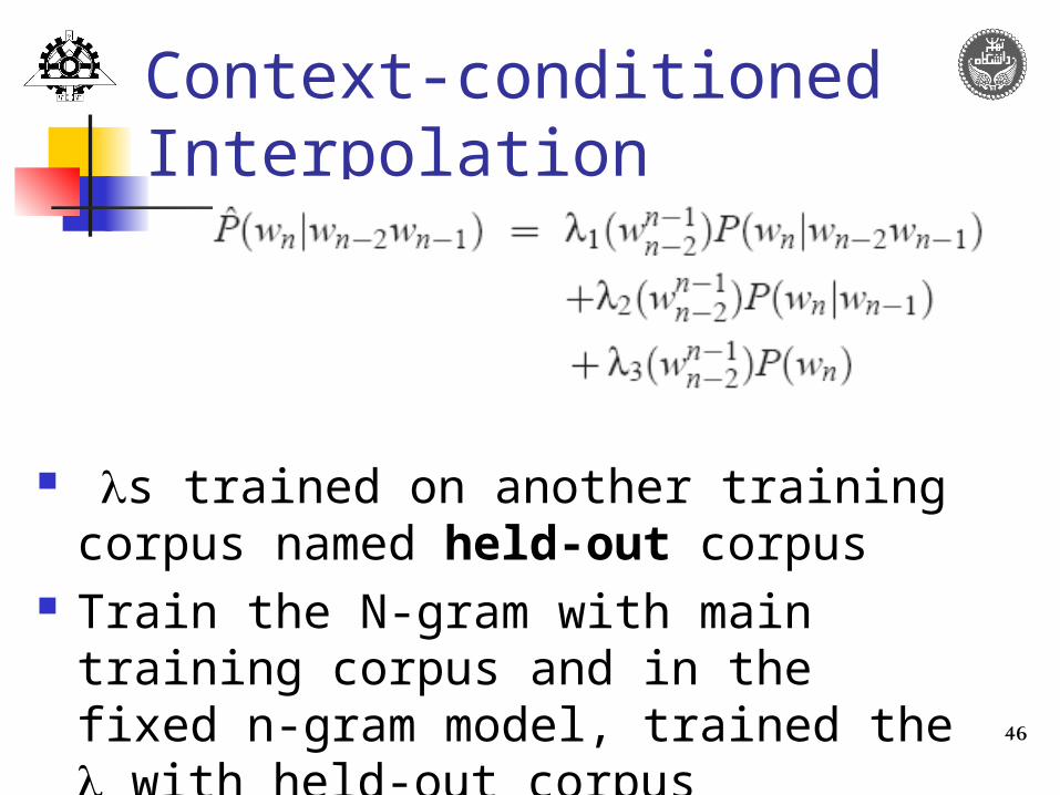
Context-conditioned Interpolation
s trained on another training corpus named held-out corpus
Train the N-gram with main training corpus and in the fixed n-gram model, trained the with held-out corpus

47
Class-based N-grams
Use information about the word classes (clusters) instead of words Instead of using “to Shanghai” use
“to London”, “to Beijing”, … , “to CITIES”
IBM Clustering P(wi|Wi-1) P(Ci|Ci-1) . P(wi|Ci)
48
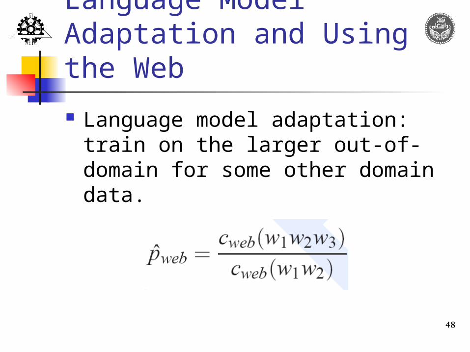
Language Model Adaptation and Using the Web
Language model adaptation: train on the larger out-of-domain for some other domain data.

49
Information Theory Another view of Perplexity is Information theory
and cross entropy Entropy is a measure of information, ENTROPY
and is invaluable throughout speech and language processing
It can be used as a metric for how much information there is in a particular grammar, for how well a given grammar matches a given language, for how predictive a given N-gram grammar is about what the next word could be.
to compare how difficult two speech recognition tasks are, and also to measure how well a given probabilistic grammar matches human grammars
50
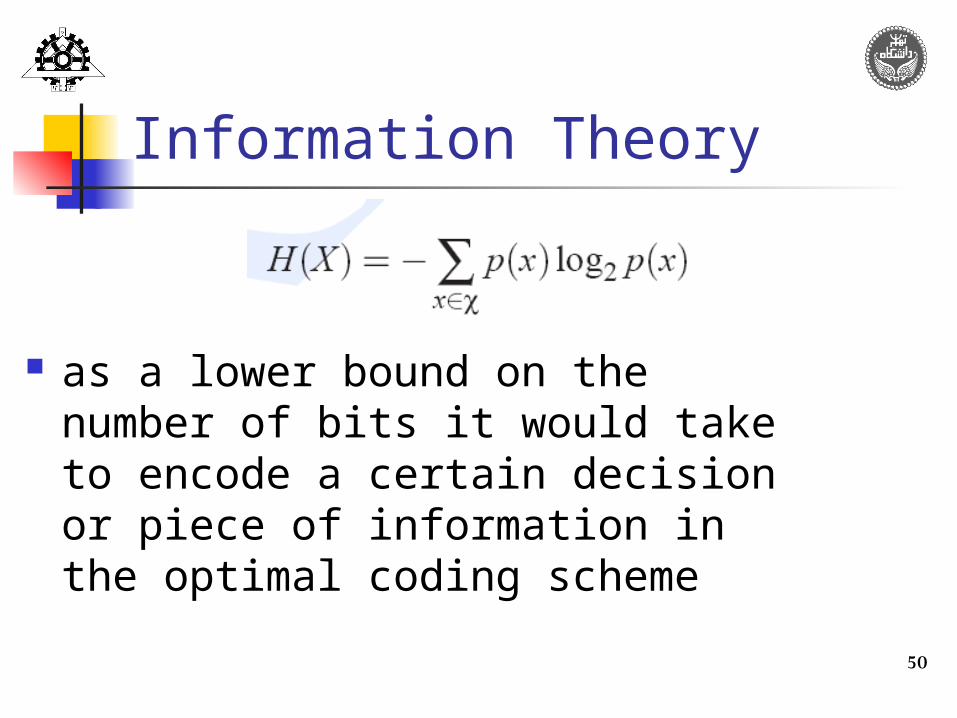
Information Theory
as a lower bound on the number of bits it would take to encode a certain decision or piece of information in the optimal coding scheme
51
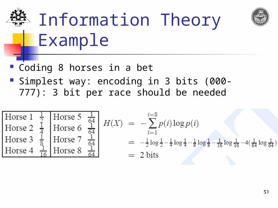
Information Theory Example
Coding 8 horses in a bet Simplest way: encoding in 3 bits (000-
777): 3 bit per race should be needed

52
Information Theory Example 0, 10, 110, 1110, 11110,111110,111111 For equal probabilities:
53
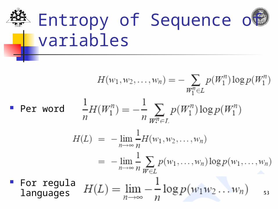
Entropy of Sequence of variables
Per word
For regular languages

54
Cross Entropy
Useful in comparing different probabilistic models
The cross-entropy is useful when we don’t know the actual probability distribution p that generated some data. Use m which is a model of p
(approximate of P)

55
Cross Entropy For some regular languages
cross entropy H(p,m) is an upper bound on the entropy H(p)
Between two models m1 and m2, the more accurate model will be the one with the lower cross-entropy

56
Cross Entropy
Approximation to the cross-entropy