Chapter 4. J2 Plasticity Algorithms v1.0
72
Computational Solid Mechanics Computational Plasticity C. Agelet de Saracibar ETS Ingenieros de Caminos, Canales y Puertos, Universidad Politécnica de Cataluña (UPC), Barcelona, Spain International Center for Numerical Methods in Engineering (CIMNE), Barcelona, Spain Chapter 4. J2 Plasticity Algorithms
-
Upload
carlos-agelet-de-saracibar -
Category
Documents
-
view
20 -
download
1
description
Computational Solid MechanicsComputational PlasticityJ2 Plasticity Algorithms
Transcript of Chapter 4. J2 Plasticity Algorithms v1.0

Computational Solid Mechanics Computational Plasticity
C. Agelet de Saracibar ETS Ingenieros de Caminos, Canales y Puertos, Universidad Politécnica de Cataluña (UPC), Barcelona, Spain
International Center for Numerical Methods in Engineering (CIMNE), Barcelona, Spain
Chapter 4. J2 Plasticity Algorithms

Contents 1. Introduction 2. J2 Rate independent plasticity models
1. Return mapping algorithm 2. Consistent elastoplastic tangent operator 3. Step by step algorithm 4. Nonlinear isotropic hardening
3. J2 Rate dependent plasticity models 1. Return mapping algorithm 2. Consistent elastoplastic tangent operator 3. Step by step algorithm 4. Nonlinear isotropic hardening
4. J2 Computational plasticity assignment
J2 Plasticity Algorithms > Contents
Contents
April 1, 2015 Carlos Agelet de Saracibar 2

Contents 1. Introduction 2. J2 Rate independent plasticity models
1. Return mapping algorithm 2. Consistent elastoplastic tangent operator 3. Step by step algorithm 4. Nonlinear isotropic hardening
3. J2 Rate dependent plasticity models 1. Return mapping algorithm 2. Consistent elastoplastic tangent operator 3. Step by step algorithm 4. Nonlinear isotropic hardening
4. J2 Computational plasticity assignment
J2 Plasticity Algorithms > Contents
Contents
April 1, 2015 Carlos Agelet de Saracibar 3

J2 Plasticity Algorithms > Introduction
Time integration algorithm
April 1, 2015 Carlos Agelet de Saracibar 4
pnE 1
pn+E
1n+E
Time integration algorithm

Contents 1. Introduction 2. J2 Rate independent plasticity models
1. Return mapping algorithm 2. Consistent elastoplastic tangent operator 3. Step by step algorithm 4. Nonlinear isotropic hardening
3. J2 Rate dependent plasticity models 1. Return mapping algorithm 2. Consistent elastoplastic tangent operator 3. Step by step algorithm 4. Nonlinear isotropic hardening
4. J2 Computational plasticity assignment
J2 Plasticity Algorithms > Contents
Contents
April 1, 2015 Carlos Agelet de Saracibar 5

1. Additive split of strains
2. Constitutive equations
3. Associative plastic flow rule
4. Yield function
5. Kuhn-Tucker loading/unloading conditions
J2 Plasticity Algorithms > Rate Independent Plasticity Models
J2 Rate independent plasticity model
April 1, 2015 Carlos Agelet de Saracibar 6
( ) { } { }23, , , diag , ,e
e e q K Hψ= ∂ = = σ q 1E
S E CE S: , C :=
{ } { } { }: : ,0,0 , : , , , : , ,e p p p e eξ ξ= + = = = − −ε ε ξ ε ξE E E , E E E
( )p fγ= ∂
SE S
( ) ( ) ( )23
: , , : dev 0Yf f q qσ= = − − − =σ q σ qS
( ) ( )0, 0, 0f fγ γ≥ ≤ =S S

Associative plastic flow rule: plastic strains at time n+1
Using a Backward-Euler (BE) time integration scheme yields,
J2 Plasticity Algorithms > Rate Independent Plasticity Models
Return mapping algorithm
April 1, 2015 Carlos Agelet de Saracibar 7
( )p fγ= ∂
SE S
( )11 1 1n
p pn n n nfγ
++ + += + ∂SE E S
1 1 1
1 1
1 1 1
2 3
p pn n n n
n n n
n n n n
γ
ξ ξ γ
γ
+ + +
+ +
+ + +
= + = + = −
ε ε n
ξ ξ n

Constitutive equations: stress state at time n+1
The time-discrete constituve equation at time n+1 takes the form,
Substituting the plastic strains at time n+1 yields,
J2 Plasticity Algorithms > Rate Independent Plasticity Models
Return mapping algorithm
April 1, 2015 Carlos Agelet de Saracibar 8
( ) ( ) { }23, diag , ,e
e e p K Hψ= ∂ = = − 1E
S E CE C E E C :=
( )1 1 1 1e p
n n n n+ + + += = −S CE C E E
( )( )( ) ( )
1
1
1 1 1 1
1 1 1
n
n
pn n n n n
pn n n n
f
f
γ
γ+
+
+ + + +
+ + +
= − − ∂
= − − ∂
S
S
S C E E S
C E E C S

Trial state at time n+1 The trial state at time n+1 is defined by freezing the plastic behaviour at the time step
J2 Plasticity Algorithms > Rate Independent Plasticity Models
Return mapping algorithm
April 1, 2015 Carlos Agelet de Saracibar 9
( ) ( )( )
,1
, ,1 1 1
, ,1 1 1 1 1
1 1
:
:
:
:
p trial pn ne trial p trialn n n
trial e trial p trial pn n n n n n
trial trialn nf f
+
+ + +
+ + + + +
+ +
=
= −
= = − = −
=
E E
E E E
S CE C E E C E E
S
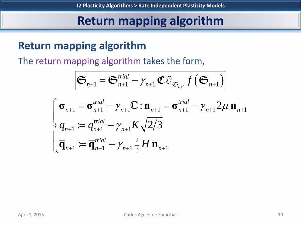
Return mapping algorithm The return mapping algorithm takes the form,
J2 Plasticity Algorithms > Rate Independent Plasticity Models
Return mapping algorithm
April 1, 2015 Carlos Agelet de Saracibar 10
( )11 1 1 1n
trialn n n nfγ
++ + + += − ∂SS S C S
1 1 1 1 1 1 1
1 1 1
21 1 1 13
: 2
: 2 3
:
trial trialn n n n n n n
trialn n n
trialn n n n
q q K
H
γ γ µ
γ
γ
+ + + + + + +
+ + +
+ + + +
= − = − = − = +
σ σ n σ n
q q n
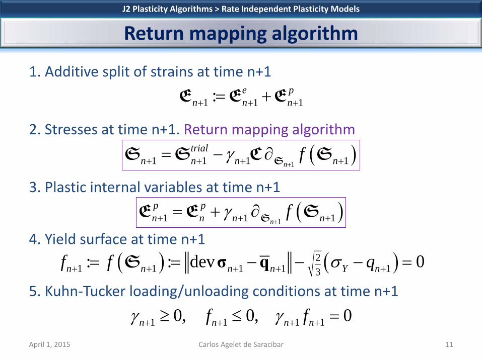
1. Additive split of strains at time n+1
2. Stresses at time n+1. Return mapping algorithm
3. Plastic internal variables at time n+1
4. Yield surface at time n+1
5. Kuhn-Tucker loading/unloading conditions at time n+1
J2 Plasticity Algorithms > Rate Independent Plasticity Models
Return mapping algorithm
April 1, 2015 Carlos Agelet de Saracibar 11
( ) ( )21 1 1 1 13: : dev 0n n n n Y nf f qσ+ + + + += = − − − =σ qS
1 1 1 10, 0, 0n n n nf fγ γ+ + + +≥ ≤ =
( )11 1 1 1n
trialn n n nfγ
++ + + += − ∂SS S C S
1 1 1: e pn n n+ + += +E E E
( )11 1 1n
p pn n n nfγ
++ + += + ∂SE E S

Theorem 1. Elastic step/plastic step If the yield function is convex and the constitutive matrix is definite-positive, the following condition holds,
and Kuhn-Tucker loading/unloading conditions can be decided just in terms of the trial state according to,
J2 Plasticity Algorithms > Rate Independent Plasticity Models
Return mapping algorithm
April 1, 2015 Carlos Agelet de Saracibar 12
( ) ( )1 1trialn nf f+ +≥S S
( )( )
1 1
1 1
Elastic step
Plastic s
0 0
0 t0 ep
trialn n
trialn n
f
f
γ
γ
+ +
+ +
< ⇒ =
> ⇒ >
S
S

Theorem 2. Closest-point-projection The stress state at time n+1 is the closest-point-projection of the trial stress state at n+1 onto the space of admissible stresses, measured in the complementary energy norm, where the complementary energy is given by,
J2 Plasticity Algorithms > Rate Independent Plasticity Models
Return mapping algorithm
April 1, 2015 Carlos Agelet de Saracibar 15
( )1 1arg min trialn n σ+ += Ξ − ∀ ∈S S S S E
( )( ) ( )
1
211 12
1 11 12
trial trialn n
trial trialn n
−+ +
−+ +
Ξ − = −
= − −C
S S S S
S S C S S

Return mapping algorithm The return mapping algorithm takes the form,
J2 Plasticity Algorithms > Rate Independent Plasticity Models
Return mapping algorithm
April 1, 2015 Carlos Agelet de Saracibar 18
( )11 1 1 1n
trialn n n nfγ
++ + + += − ∂SS S C S
1 1 1 1 1 1 1
1 1 1
21 1 1 13
: 2
: 2 3
:
trial trialn n n n n n n
trialn n n
trialn n n n
q q K
H
γ γ µ
γ
γ
+ + + + + + +
+ + +
+ + + +
= − = − = − = +
σ σ n σ n
q q n

The solution for the return mapping algorithm yields,
J2 Plasticity Algorithms > Rate Independent Plasticity Models
Return mapping algorithm
April 1, 2015 Carlos Agelet de Saracibar 19
( )21 1 1 1 1 132trial trial
n n n n n nHγ µ+ + + + + +− = − − +σ q σ q n
( )21 1 1 1 1 1 1 132trial trial trial
n n n n n n n nHγ µ+ + + + + + + +− = − − +σ q n σ q n n
( )( )21 1 1 1 1 1 132 trial trial trial
n n n n n n nHγ µ+ + + + + + +− + + = −σ q n σ q n
( )21 1 1 1 13
1 1
2 trial trialn n n n n
trialn n
Hγ µ+ + + + +
+ +
− + + = −
=
σ q σ q
n n

For the non-trivial case (plastic loading), using the discrete Kuhn-Tucker loading/unloading conditions, the discrete plastic multiplier (or discrete plastic consistency parameter) reads,
J2 Plasticity Algorithms > Rate Independent Plasticity Models
Return mapping algorithm
April 1, 2015 Carlos Agelet de Saracibar 20
( )1 1 1 1if 0 then , , 0n n n nf qγ + + + +> =σ q
( ) ( )
( ) ( )( ) ( )
21 1 1 1 1 13
2 2 21 1 1 13 3 3
2 21 1 1 1 3 3
, , dev
2
, , 2 0
n n n n n Y n
trial trial trialn n n Y n
trial trial trialn n n n
f q q
K H q
f q K H
σ
γ µ σ
γ µ
+ + + + + +
+ + + +
+ + + +
= − − −
= − − + + − −
= − + + =
σ q σ q
σ q
σ q
( ) 12 21 13 32 trial
n nK H fγ µ−
+ += + +
( ) ( )1 1 1 1 1 1 1 10, , , 0, , , 0n n n n n n n nf q f qγ γ+ + + + + + + +≥ ≤ =σ q σ q

The return mapping algorithm takes the form,
J2 Plasticity Algorithms > Rate Independent Plasticity Models
Return mapping algorithm
April 1, 2015 Carlos Agelet de Saracibar 21
( )( )( )
12 21 1 1 13 3
12 21 1 13 3
12 21 1 1 13 3
2 2
: 2 2 3
2: 23
trial trial trialn n n n
trial trialn n n
trial trial trialn n n n
K H f
q q K H f K
K H f H
µ µ
µ
µ
−
+ + + +
−
+ + +
−
+ + + +
= − + +
= − + + = + + +
σ σ n
q q n
1 1 1 1 1 1 1
1 1 1
21 1 1 13
: 2
: 2 3
:
trial trialn n n n n n n
trialn n n
trialn n n n
q q K
H
γ γ µ
γ
γ
+ + + + + + +
+ + +
+ + + +
= − = − = − = +
σ σ n σ n
q q n

Return mapping algorithm: Geometric interpretation
J2 Plasticity Algorithms > Rate Independent Plasticity Models
Return mapping algorithm
April 1, 2015 Carlos Agelet de Saracibar 22
, 1nσ +
1dev n+σ
1n+q
( )1 1
23n nYR qσ+ += −
1n+n
1dev trialn+σ
dev nσ
,nσnq
( )23n nYR qσ= −
1trialn+n

The update of the plastic internal variables takes the form,
J2 Plasticity Algorithms > Rate Independent Plasticity Models
Return mapping algorithm
April 1, 2015 Carlos Agelet de Saracibar 23
1 1 1
1 1
1 1 1
2 3
p pn n n n
n n n
n n n n
γ
ξ ξ γ
γ
+ + +
+ +
+ + +
= + = + = −
ε ε n
ξ ξ n
( )( )( )
12 21 1 13 3
12 21 13 3
12 21 1 13 3
2
2 2 3
2
p p trial trialn n n n
trialn n n
trial trialn n n n
K H f
K H f
K H f
µ
ξ ξ µ
µ
−
+ + +
−
+ +
−
+ + +
= + + + = + + + = − + +
ε ε n
ξ ξ n
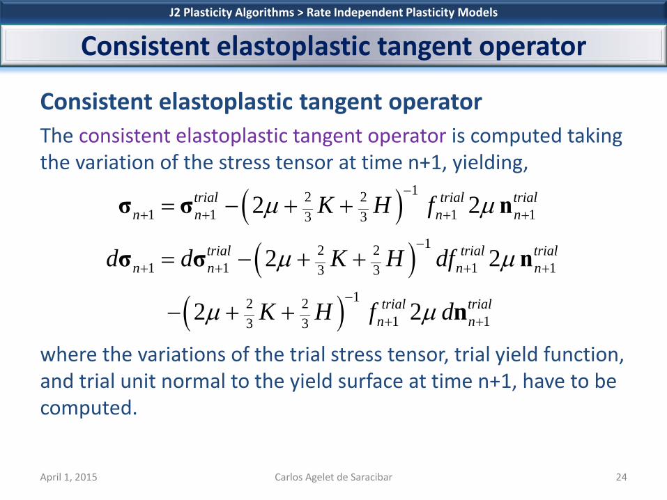
Consistent elastoplastic tangent operator The consistent elastoplastic tangent operator is computed taking the variation of the stress tensor at time n+1, yielding, where the variations of the trial stress tensor, trial yield function, and trial unit normal to the yield surface at time n+1, have to be computed.
J2 Plasticity Algorithms > Rate Independent Plasticity Models
Consistent elastoplastic tangent operator
April 1, 2015 Carlos Agelet de Saracibar 24
( )( )
( )
12 21 1 1 13 3
12 21 1 1 13 3
12 21 13 3
2 2
2 2
2 2
trial trial trialn n n n
trial trial trialn n n n
trial trialn n
K H f
d d K H df
K H f d
µ µ
µ µ
µ µ
−
+ + + +
−
+ + + +
−
+ +
= − + +
= − + +
− + +
σ σ n
σ σ n
n

The variation of the trial stress tensor at time n+1 takes the form,
J2 Plasticity Algorithms > Rate Independent Plasticity Models
Consistent elastoplastic tangent operator
April 1, 2015 Carlos Agelet de Saracibar 25
( ) ( )( ) ( ) ( ) ( )( ) ( )( )
1 1 1 1 1
1 1 1 1
1 1 1 1 1
1 1
tr 2 tr 2 dev
tr 2 tr 2 dev
tr 2 tr 2 dev
tr 2
trial etrial etrial etrial etrialn n n n n
p pn n n n n n
trial etrial etrial etrial etrialn n n n n
n n
d d d
d d
λ µ κ µ
λ µ κ µ
λ µ κ µ
λ µ
+ + + + +
+ + + +
+ + + + +
+ +
= + = +
= + − = + −
= + = +
= +
σ ε 1 ε ε 1 ε
ε 1 ε ε ε 1 ε ε
σ ε 1 ε ε 1 ε
ε 1 ε ( )( ) ( ) ( )( )
1 1
11 1 13
tr 2 dev
: 2 2 :
n n
n n n
d d
d d d
κ µ
λ µ κ µ
+ +
+ + +
= +
= ⊗ + = ⊗ + − ⊗
ε 1 ε
1 1 ε ε 1 1 1 1 ε
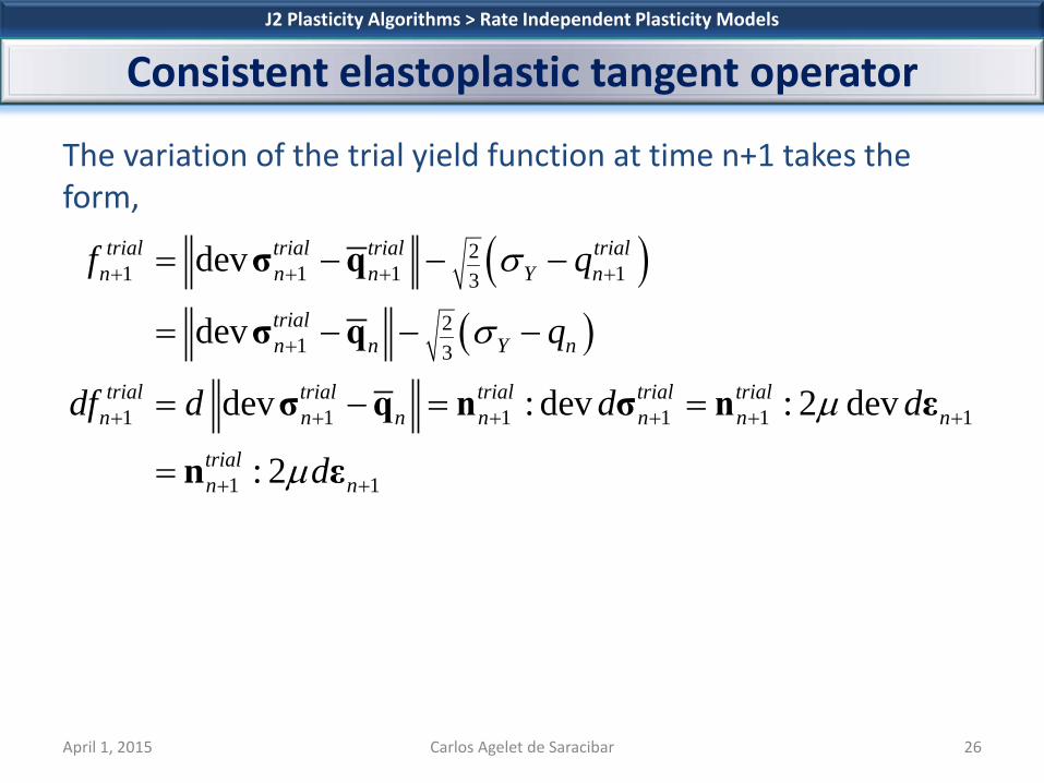
The variation of the trial yield function at time n+1 takes the form,
J2 Plasticity Algorithms > Rate Independent Plasticity Models
Consistent elastoplastic tangent operator
April 1, 2015 Carlos Agelet de Saracibar 26
( )( )
21 1 1 13
21 3
1 1 1 1 1 1
1 1
dev
dev
dev : dev : 2 dev
: 2
trial trial trial trialn n n Y n
trialn n Y n
trial trial trial trial trialn n n n n n n
trialn n
f q
q
df d d d
d
σ
σ
µ
µ
+ + + +
+
+ + + + + +
+ +
= − − −
= − − −
= − = =
=
σ q
σ q
σ q n σ n ε
n ε

The variation of the unit normal to the yield surface at time n+1 takes the form,
J2 Plasticity Algorithms > Rate Independent Plasticity Models
Consistent elastoplastic tangent operator
April 1, 2015 Carlos Agelet de Saracibar 27
( )( )
1 1 11
1 1 1
11 1 1 1dev 1
11 1 1dev 1
dev devdev dev
dev dev
: dev
trial trial trialtrial n n n nn trial trial trial
n n n n
trial trial trial trialn n n n ntrial
n n
trial trial trn n ntrial
n n
d d d
d
+ + ++
+ + +
+ + + +−+
+ + +−+
− −= =
− −
= − −
= − ⊗
σ q
σ q
σ q σ qnσ q σ q
n σ n σ q
n n σ
( )11 1 1dev 1
11 1 1dev 1
: 2 dev
1 : 23
ial
trial trialn n ntrial
n n
trial trialn n ntrial
n n
d
d
µ
µ
+ + +−+
+ + +−+
= − ⊗
= − ⊗ − ⊗
σ q
σ q
n n ε
1 1 n n ε
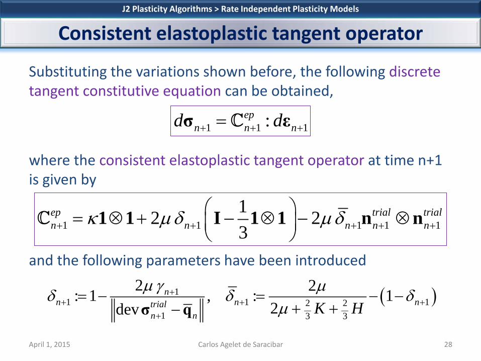
Substituting the variations shown before, the following discrete tangent constitutive equation can be obtained, where the consistent elastoplastic tangent operator at time n+1 is given by
and the following parameters have been introduced
J2 Plasticity Algorithms > Rate Independent Plasticity Models
Consistent elastoplastic tangent operator
April 1, 2015 Carlos Agelet de Saracibar 28
1 1 1:epn n nd d+ + +=σ ε
1 1 1 1 112 23
ep trial trialn n n n nκ µδ µδ+ + + + +
= ⊗ + − ⊗ − ⊗
1 1 I 1 1 n n
( )11 1 12 2
1 3 3
2 2: 1 , : 12dev
nn n ntrial
n n K Hµ γ µδ δ δ
µ+
+ + ++
= − = − −+ +−σ q

J2 Plasticity algorithm Step 1. Given the strain tensor at time n+1 (strain driven problem), and the stored plastic internal variables at time n (plastic internal variables database) Step 2. Compute the trial state at time n+1
J2 Plasticity Algorithms > Rate Independent Plasticity Models
J2 Plasticity algorithm
April 1, 2015 Carlos Agelet de Saracibar 29
( ) ( )( )
,1
, ,1 1 1
, ,1 1 1 1 1
21 1 1 13
:
:
:
: dev
p trial pn ne trial p trialn n n
trial e trial p trial pn n n n n n
trial trial trial trialn n n Y nf qσ
+
+ + +
+ + + + +
+ + + +
=
= −
= = − = −
= − − −σ q
E E
E E E
S CE C E E C E E

Step 3. Check the trial yield function at time n+1 Step 4. Compute the discrete plastic multiplier at time n+1
J2 Plasticity Algorithms > Rate Independent Plasticity Models
J2 Plasticity algorithm
April 1, 2015 Carlos Agelet de Saracibar 30
( ) ( )1 11 1if 0 then set , and exittrialtrial ep
n nn nf + ++ +
≤ • = • =
( ) 12 21 13 32 trial
n nK H fγ µ−
+ += + +

Step 5. Return mapping algorithm (closest-point-projection)
J2 Plasticity Algorithms > Rate Independent Plasticity Models
J2 Plasticity algorithm
April 1, 2015 Carlos Agelet de Saracibar 31
( )1
1 1 1 1trialn
trial trialn n n nfγ
++ + + += − ∂
SS S C S
( )( )( )
12 21 1 1 13 3
12 21 1 13 3
12 21 1 1 13 3
2 2
: 2 2 3
2: 23
trial trial trialn n n n
trial trialn n n
trial trial trialn n n n
K H f
q q K H f K
K H f H
µ µ
µ
µ
−
+ + + +
−
+ + +
−
+ + + +
= − + +
= − + + = + + +
σ σ n
q q n
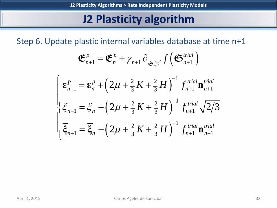
Step 6. Update plastic internal variables database at time n+1
J2 Plasticity Algorithms > Rate Independent Plasticity Models
J2 Plasticity algorithm
April 1, 2015 Carlos Agelet de Saracibar 32
( )1
1 1 1trialn
p p trialn n n nfγ
++ + += + ∂
SE E S
( )( )( )
12 21 1 13 3
12 21 13 3
12 21 1 13 3
2
2 2 3
2
p p trial trialn n n n
trialn n n
trial trialn n n n
K H f
K H f
K H f
µ
ξ ξ µ
µ
−
+ + +
−
+ +
−
+ + +
= + + + = + + + = − + +
ε ε n
ξ ξ n
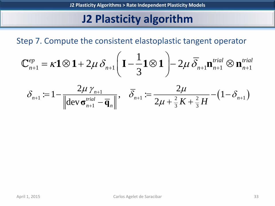
Step 7. Compute the consistent elastoplastic tangent operator
J2 Plasticity Algorithms > Rate Independent Plasticity Models
J2 Plasticity algorithm
April 1, 2015 Carlos Agelet de Saracibar 33
1 1 1 1 112 23
ep trial trialn n n n nκ µδ µδ+ + + + +
= ⊗ + − ⊗ − ⊗
1 1 I 1 1 n n
( )11 1 12 2
1 3 3
2 2: 1 , : 12dev
nn n ntrial
n n K Hµ γ µδ δ δ
µ+
+ + ++
= − = − −+ +−σ q
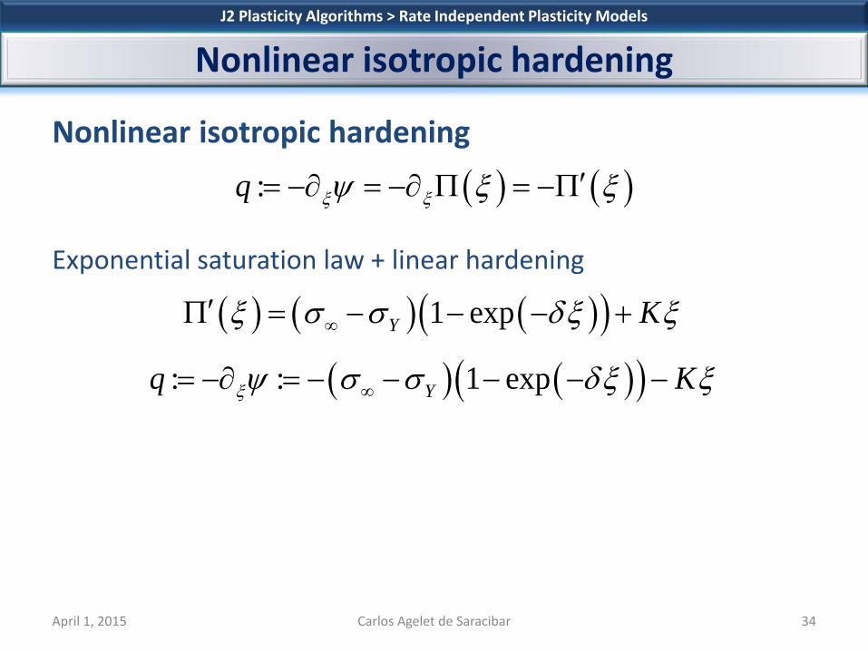
Nonlinear isotropic hardening Exponential saturation law + linear hardening
J2 Plasticity Algorithms > Rate Independent Plasticity Models
Nonlinear isotropic hardening
April 1, 2015 Carlos Agelet de Saracibar 34
( ) ( ):q ξ ξψ ξ ξ′= −∂ = −∂ Π = −Π
( ) ( )( ): : 1 expYq Kξψ σ σ δξ ξ∞= −∂ = − − − − −
( ) ( ) ( )( )1 expY Kξ σ σ δξ ξ∞′Π = − − − +

Time discrete nonlinear isotropic hardening
J2 Plasticity Algorithms > Rate Independent Plasticity Models
Nonlinear isotropic hardening
April 1, 2015 Carlos Agelet de Saracibar 35
( ) ( )( ) ( )
( ) ( )
1 1 1
1 1
1 1 1
: 2 3
:
: 2 3
n n n n
trial trialn n n n
trialn n n n n
q
q q
q q
ξ ξ γ
ξ ξ
ξ γ ξ
+ + +
+ +
+ + +
′ ′= −Π = −Π +
′ ′= −Π = −Π =
′ ′= −Π + +Π
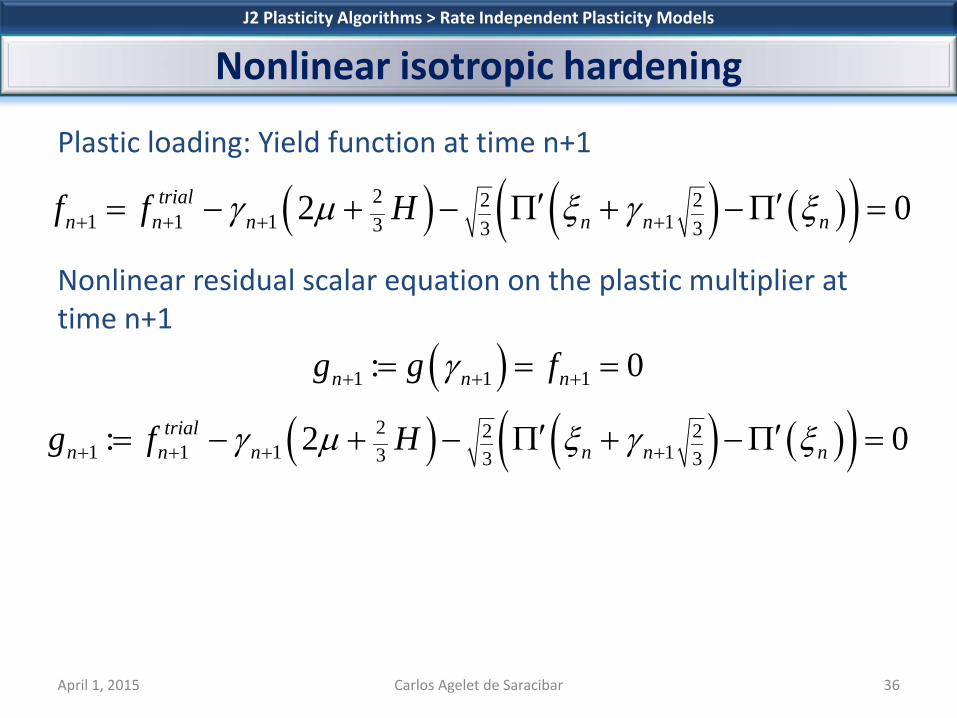
Plastic loading: Yield function at time n+1 Nonlinear residual scalar equation on the plastic multiplier at time n+1
J2 Plasticity Algorithms > Rate Independent Plasticity Models
Nonlinear isotropic hardening
April 1, 2015 Carlos Agelet de Saracibar 36
( ) ( ) ( )( )2 2 21 1 1 13 3 3
2 0trialn n n n n nf f Hγ µ ξ γ ξ+ + + +′ ′= − + − Π + −Π =
( )( ) ( ) ( )( )
1 1 1
2 2 21 1 1 13 3 3
: 0
: 2 0
n n n
trialn n n n n n
g g f
g f H
γ
γ µ ξ γ ξ
+ + +
+ + + +
= = =
′ ′= − + − Π + −Π =

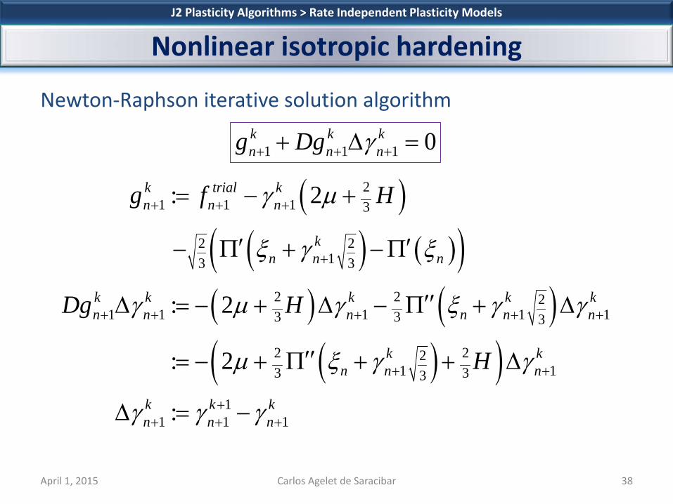
Newton-Raphson iterative solution algorithm Step 1. Initialize iteration counter and plastic multiplier Step 2. Compute the residual g at time n+1, iteration k Step 3. While the absolute value of the current residual at time n+1, iteration k, is greater than a tolerance Step 4. Solve the linarized equation Step 5. Update the plastic multiplier at time n+1, iteration k+1 Step 6. Compute the residual g at time n+1, iteration k+1 Step 7. Increment iteration counter k=k+1 and go to Step 3
J2 Plasticity Algorithms > Rate Independent Plasticity Models
Nonlinear isotropic hardening
April 1, 2015 Carlos Agelet de Saracibar 37
10, 0knk γ += =
1 1 1 0k k kn n ng Dg γ+ + ++ ∆ =
11 1 1
k k kn n nγ γ γ++ + += + ∆
Newton-Raphson iterative solution algorithm
J2 Plasticity Algorithms > Rate Independent Plasticity Models
Nonlinear isotropic hardening
April 1, 2015 Carlos Agelet de Saracibar 38
( )( ) ( )( )
( ) ( )( )( )
21 1 1 3
2 213 3
2 2 21 1 1 1 13 3 3
2 221 13 33
11 1 1
: 2
: 2
: 2
:
k trial kn n n
kn n n
k k k k kn n n n n n
k kn n n
k k kn n n
g f H
Dg H
H
γ µ
ξ γ ξ
γ µ γ ξ γ γ
µ ξ γ γ
γ γ γ
+ + +
+
+ + + + +
+ +
++ + +
= − +
′ ′− Π + −Π
′′∆ = − + ∆ − Π + ∆
′′= − + Π + + ∆
∆ = −
1 1 1 0k k kn n ng Dg γ+ + ++ ∆ =
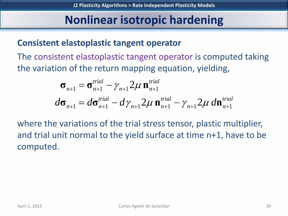
Consistent elastoplastic tangent operator The consistent elastoplastic tangent operator is computed taking the variation of the return mapping equation, yielding, where the variations of the trial stress tensor, plastic multiplier, and trial unit normal to the yield surface at time n+1, have to be computed.
J2 Plasticity Algorithms > Rate Independent Plasticity Models
Nonlinear isotropic hardening
April 1, 2015 Carlos Agelet de Saracibar 39
1 1 1 1
1 1 1 1 1 1
2
2 2
trial trialn n n n
trial trial trialn n n n n nd d d d
γ µ
γ µ γ µ+ + + +
+ + + + + +
= −
= − −
σ σ nσ σ n n

The variation of the plastic multiplier at time n+1 is computed setting the variation of the residual equal to zero,
J2 Plasticity Algorithms > Rate Independent Plasticity Models
Nonlinear isotropic hardening
April 1, 2015 Carlos Agelet de Saracibar 40
( ) ( ) ( )( )( ) ( )
( )( )( )( )
2 2 21 1 1 13 3 3
2 2 21 1 1 1 13 3 3
2 221 1 13 33
12 22
1 1 13 33
: 2
: 2
: 2 0
2
trialn n n n n n
trialn n n n n n
trialn n n n
trialn n n n
g f H
dg df d H d
df d H
d H df
γ µ ξ γ ξ
γ µ ξ γ γ
γ µ ξ γ
γ µ ξ γ
+ + + +
+ + + + +
+ + +
−
+ + +
′ ′= − + − Π + −Π
′′= − + − Π +
′′= − + Π + + =
′′= + Π + +

Substituting the variations shown before, the following discrete tangent constitutive equation can be obtained, where the consistent elastoplastic tangent operator at time n+1 is given by
and the following parameters have been introduced
J2 Plasticity Algorithms > Rate Independent Plasticity Models
Nonlinear isotropic hardening
April 1, 2015 Carlos Agelet de Saracibar 41
1 1 1:epn n nd d+ + +=σ ε
1 1 1 1 112 23
ep trial trialn n n n nκ µδ µδ+ + + + +
= ⊗ + − ⊗ − ⊗
1 1 I 1 1 n n
( ) ( )11 1 12 22
1 13 33
2 2: 1 , : 1dev 2
nn n ntrial
n n n n Hµ γ µδ δ δ
µ ξ γ+
+ + ++ +
= − = − −− ′′+ Π + +σ q
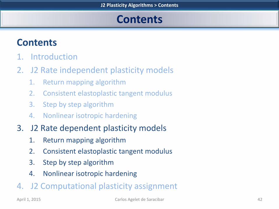
Contents 1. Introduction 2. J2 Rate independent plasticity models
1. Return mapping algorithm 2. Consistent elastoplastic tangent modulus 3. Step by step algorithm 4. Nonlinear isotropic hardening
3. J2 Rate dependent plasticity models 1. Return mapping algorithm 2. Consistent elastoplastic tangent modulus 3. Step by step algorithm 4. Nonlinear isotropic hardening
4. J2 Computational plasticity assignment
J2 Plasticity Algorithms > Contents
Contents
April 1, 2015 Carlos Agelet de Saracibar 42

1. Additive split of strains
2. Constitutive equations
3. Associative plastic flow rule
4. Yield function
5. Plastic multiplier
J2 Plasticity Algorithms > Rate Dependent Plasticity Models
J2 Rate dependent plasticity model
April 1, 2015 Carlos Agelet de Saracibar 43
( ) { } { }23, , , diag , ,e
e e q K Hψ= ∂ = = σ q 1E
S E CE S: , C :=
{ } { } { }: : ,0,0 , : , , , : , ,e p p p e eξ ξ= + = = = − −ε ε ξ ε ξE E E , E E E
( )p fγ= ∂
SE S
( ) ( ) ( )23
: , , : dev 0Yf f q qσ= = − − − =σ q σ qS
( )1 0fηγ = ≥S

Associative plastic flow rule: plastic strains at time n+1
Using a Backward-Euler (BE) time integration scheme yields,
J2 Plasticity Algorithms > Rate Dependent Plasticity Models
Return mapping algorithm
April 1, 2015 Carlos Agelet de Saracibar 44
( )p fγ= ∂
SE S
( )11 1 1n
p pn n n nt fγ
++ + += + ∆ ∂SE E S
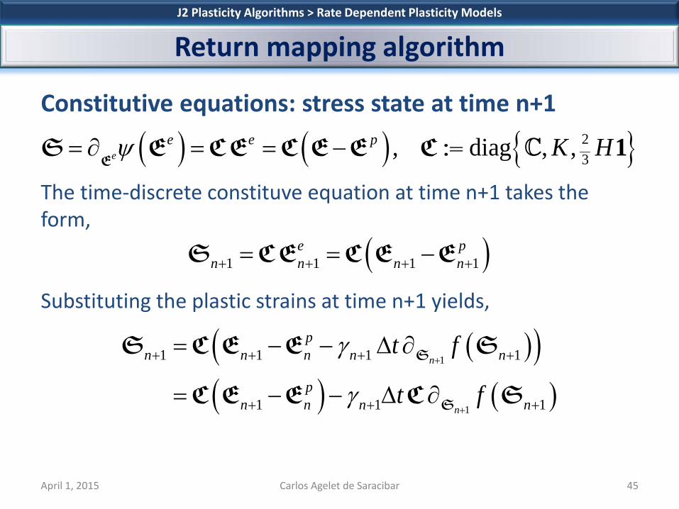
Constitutive equations: stress state at time n+1
The time-discrete constituve equation at time n+1 takes the form,
Substituting the plastic strains at time n+1 yields,
J2 Plasticity Algorithms > Rate Dependent Plasticity Models
Return mapping algorithm
April 1, 2015 Carlos Agelet de Saracibar 45
( ) ( ) { }23, diag , ,e
e e p K Hψ= ∂ = = − 1E
S E CE C E E C :=
( )1 1 1 1e p
n n n n+ + + += = −S CE C E E
( )( )( ) ( )
1
1
1 1 1 1
1 1 1
n
n
pn n n n n
pn n n n
t f
t f
γ
γ+
+
+ + + +
+ + +
= − − ∆ ∂
= − − ∆ ∂
S
S
S C E E S
C E E C S

Trial state at time n+1 The trial state at time n+1 is defined by freezing the plastic behaviour
J2 Plasticity Algorithms > Rate Dependent Plasticity Models
Return mapping algorithm
April 1, 2015 Carlos Agelet de Saracibar 46
( ) ( )( )
,1
, ,1 1 1
, ,1 1 1 1 1
1 1
:
:
:
:
p trial pn ne trial p trialn n n
trial e trial p trial pn n n n n n
trial trialn nf f
+
+ + +
+ + + + +
+ +
=
= −
= = − = −
=
E E
E E E
S CE C E E C E E
S

Return mapping algorithm The return mapping algorithm takes the form,
J2 Plasticity Algorithms > Rate Dependent Plasticity Models
Return mapping algorithm
April 1, 2015 Carlos Agelet de Saracibar 47
( )11 1 1 1n
trialn n n nt fγ
++ + + += − ∆ ∂SS S C S
1 1 1 1 1 1 1
1 1 1
21 1 1 13
: 2
: 2 3
:
trial trialn n n n n n n
trialn n n
trialn n n n
t
q q t K
t H
γ γ µ
γ
γ
+ + + + + + +
+ + +
+ + + +
= − ∆ = − = − ∆ = + ∆
σ σ n σ n
q q n
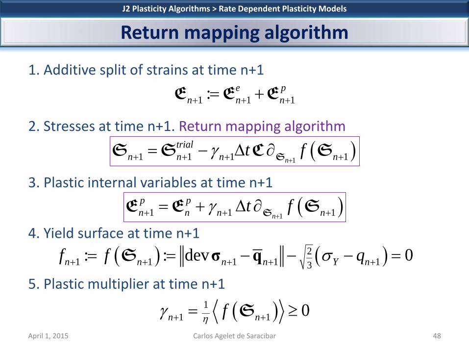
1. Additive split of strains at time n+1
2. Stresses at time n+1. Return mapping algorithm
3. Plastic internal variables at time n+1
4. Yield surface at time n+1
5. Plastic multiplier at time n+1
J2 Plasticity Algorithms > Rate Dependent Plasticity Models
Return mapping algorithm
April 1, 2015 Carlos Agelet de Saracibar 48
( ) ( )21 1 1 1 13: : dev 0n n n n Y nf f qσ+ + + + += = − − − =σ qS
( )11 1 1 1n
trialn n n nt fγ
++ + + += − ∆ ∂SS S C S
1 1 1: e pn n n+ + += +E E E
( )11 1 1n
p pn n n nt fγ
++ + += + ∆ ∂SE E S
( )11 1 0n nfηγ + += ≥S

Return mapping algorithm The return mapping algorithm takes the form,
J2 Plasticity Algorithms > Rate Dependent Plasticity Models
Return mapping algorithm
April 1, 2015 Carlos Agelet de Saracibar 49
( )11 1 1 1n
trialn n n nt fγ
++ + + += − ∆ ∂SS S C S
1 1 1 1 1 1 1
1 1 1
21 1 1 13
: 2
: 2 3
:
trial trialn n n n n n n
trialn n n
trialn n n n
t
q q t K
t H
γ γ µ
γ
γ
+ + + + + + +
+ + +
+ + + +
= − ∆ = − = − ∆ = + ∆
σ σ n σ n
q q n
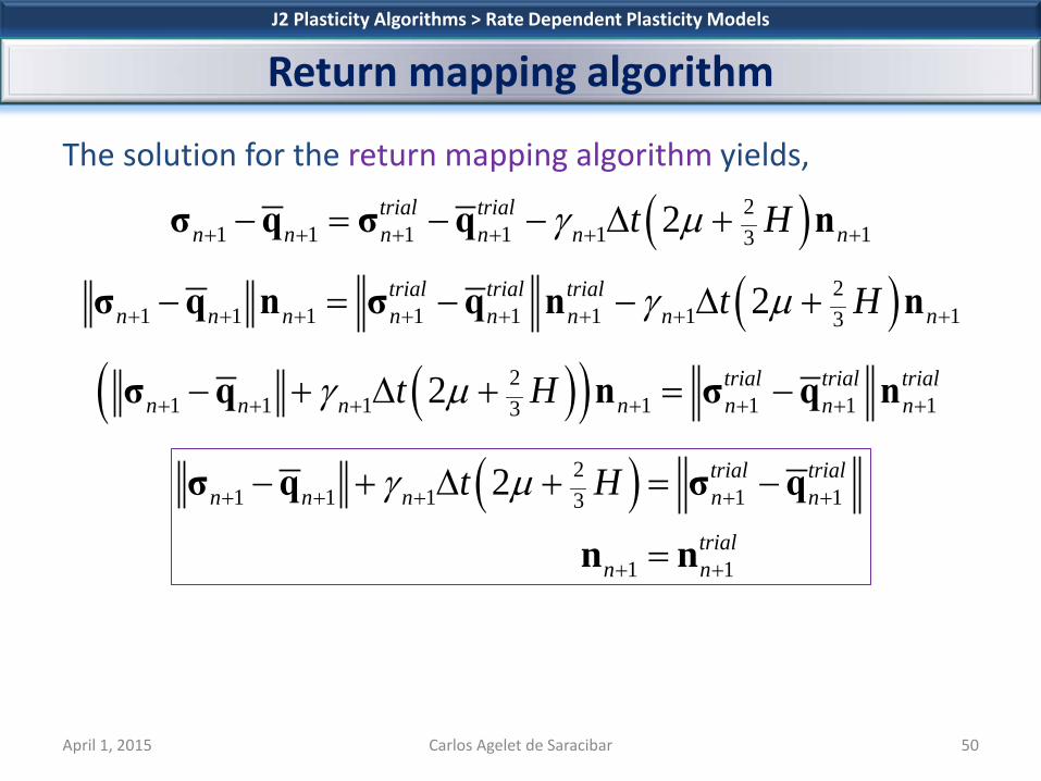
The solution for the return mapping algorithm yields,
J2 Plasticity Algorithms > Rate Dependent Plasticity Models
Return mapping algorithm
April 1, 2015 Carlos Agelet de Saracibar 50
( )21 1 1 1 1 132trial trial
n n n n n nt Hγ µ+ + + + + +− = − − ∆ +σ q σ q n
( )21 1 1 1 1 1 1 132trial trial trial
n n n n n n n nt Hγ µ+ + + + + + + +− = − − ∆ +σ q n σ q n n
( )( )21 1 1 1 1 1 132 trial trial trial
n n n n n n nt Hγ µ+ + + + + + +− + ∆ + = −σ q n σ q n
( )21 1 1 1 13
1 1
2 trial trialn n n n n
trialn n
t Hγ µ+ + + + +
+ +
− + ∆ + = −
=
σ q σ q
n n

For the non-trivial case (plastic loading), the discrete plastic multiplier reads,
J2 Plasticity Algorithms > Rate Dependent Plasticity Models
Return mapping algorithm
April 1, 2015 Carlos Agelet de Saracibar 51
( )1 1 1 1 1if 0 then , ,n n n n nf qγ γ η+ + + + +> =σ q
( ) ( )
( ) ( )( ) ( )
21 1 1 1 1 13
2 2 21 1 1 13 3 3
2 21 1 1 1 13 3
, , dev
2
, , 2
n n n n n Y n
trial trial trialn n n Y n
trial trial trialn n n n n
f q q
t K H q
f q t K H
σ
γ µ σ
γ µ γ η
+ + + + + +
+ + + +
+ + + + +
= − − −
= − − ∆ + + − −
= − ∆ + + =
σ q σ q
σ q
σ q
12 2
1 13 32 trialn nt K H f
tηγ µ
−
+ + ∆ = + + + ∆

The return mapping algorithm takes the form,
J2 Plasticity Algorithms > Rate Dependent Plasticity Models
Return mapping algorithm
April 1, 2015 Carlos Agelet de Saracibar 52
12 2
1 1 1 13 3
12 2
1 1 13 3
12 2
1 1 1 13 3
2 2
: 2 2 3
2: 23
trial trial trialn n n n
trial trialn n n
trial trial trialn n n n
K H ft
q q K H f Kt
K H f Ht
ηµ µ
ηµ
ηµ
−
+ + + +
−
+ + +
−
+ + + +
= − + + + ∆ = − + + + ∆ = + + + + ∆
σ σ n
q q n
1 1 1 1 1 1 1
1 1 1
21 1 1 13
: 2
: 2 3
:
trial trialn n n n n n n
trialn n n
trialn n n n
t
q q t K
t H
γ γ µ
γ
γ
+ + + + + + +
+ + +
+ + + +
= − ∆ = − = − ∆ = + ∆
σ σ n σ n
q q n

The update of the plastic internal variables takes the form,
J2 Plasticity Algorithms > Rate Dependent Plasticity Models
Return mapping algorithm
April 1, 2015 Carlos Agelet de Saracibar 53
1 1 1
1 1
1 1 1
2 3
p pn n n n
n n n
n n n n
t
t
t
γ
ξ ξ γ
γ
+ + +
+ +
+ + +
= + ∆ = + ∆ = − ∆
ε ε n
ξ ξ n1
2 21 1 13 3
12 2
1 13 3
12 2
1 1 13 3
2
2 2 3
2
p p trial trialn n n n
trialn n n
trial trialn n n n
K H ft
K H ft
K H ft
ηµ
ηξ ξ µ
ηµ
−
+ + +
−
+ +
−
+ + +
= + + + + ∆ = + + + + ∆ = − + + + ∆
ε ε n
ξ ξ n
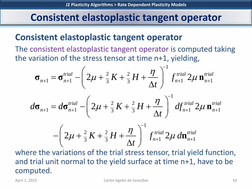
Consistent elastoplastic tangent operator The consistent elastoplastic tangent operator is computed taking the variation of the stress tensor at time n+1, yielding,
where the variations of the trial stress tensor, trial yield function, and trial unit normal to the yield surface at time n+1, have to be computed.
J2 Plasticity Algorithms > Rate Dependent Plasticity Models
Consistent elastoplastic tangent operator
April 1, 2015 Carlos Agelet de Saracibar 54
12 2
1 1 1 13 3
12 2
1 1 1 13 3
12 2
1 13 3
2 2
2 2
2 2
trial trial trialn n n n
trial trial trialn n n n
trial trialn n
K H ft
d d K H dft
K H f dt
ηµ µ
ηµ µ
ηµ µ
−
+ + + +
−
+ + + +
−
+ +
= − + + + ∆
= − + + + ∆
− + + + ∆
σ σ n
σ σ n
n

The variation of the trial stress tensor at time n+1 takes the form,
J2 Plasticity Algorithms > Rate Dependent Plasticity Models
Consistent elastoplastic tangent operator
April 1, 2015 Carlos Agelet de Saracibar 55
( ) ( )( ) ( ) ( ) ( )( ) ( )( )
1 1 1 1 1
1 1 1 1
1 1 1 1 1
1 1
tr 2 tr 2 dev
tr 2 tr 2 dev
tr 2 tr 2 dev
tr 2
trial etrial etrial etrial etrialn n n n n
p pn n n n n n
trial etrial etrial etrial etrialn n n n n
n n
d d d
d d
λ µ κ µ
λ µ κ µ
λ µ κ µ
λ µ
+ + + + +
+ + + +
+ + + + +
+ +
= + = +
= + − = + −
= + = +
= +
σ ε 1 ε ε 1 ε
ε 1 ε ε ε 1 ε ε
σ ε 1 ε ε 1 ε
ε 1 ε ( )( ) ( ) ( )( )
1 1
11 1 13
tr 2 dev
: 2 2 :
n n
n n n
d d
d d d
κ µ
λ µ κ µ
+ +
+ + +
= +
= ⊗ + = ⊗ + − ⊗
ε 1 ε
1 1 ε ε 1 1 1 1 ε

The variation of the trial yield function at time n+1 takes the form,
J2 Plasticity Algorithms > Rate Dependent Plasticity Models
Consistent elastoplastic tangent operator
April 1, 2015 Carlos Agelet de Saracibar 56
( )( )
21 1 1 13
21 3
1 1 1 1 1 1
1 1
dev
dev
dev : dev : 2 dev
: 2
trial trial trial trialn n n Y n
trialn n Y n
trial trial trial trial trialn n n n n n n
trialn n
f q
q
df d d d
d
σ
σ
µ
µ
+ + + +
+
+ + + + + +
+ +
= − − −
= − − −
= − = =
=
σ q
σ q
σ q n σ n ε
n ε
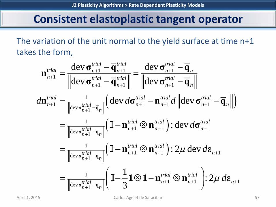
The variation of the unit normal to the yield surface at time n+1 takes the form,
J2 Plasticity Algorithms > Rate Dependent Plasticity Models
Consistent elastoplastic tangent operator
April 1, 2015 Carlos Agelet de Saracibar 57
( )( )
1 1 11
1 1 1
11 1 1 1dev 1
11 1 1dev 1
dev devdev dev
dev dev
: dev
trial trial trialtrial n n n nn trial trial trial
n n n n
trial trial trial trialn n n n ntrial
n n
trial trial trn n ntrial
n n
d d d
d
+ + ++
+ + +
+ + + +−+
+ + +−+
− −= =
− −
= − −
= − ⊗
σ q
σ q
σ q σ qnσ q σ q
n σ n σ q
n n σ
( )11 1 1dev 1
11 1 1dev 1
: 2 dev
1 : 23
ial
trial trialn n ntrial
n n
trial trialn n ntrial
n n
d
d
µ
µ
+ + +−+
+ + +−+
= − ⊗
= − ⊗ − ⊗
σ q
σ q
n n ε
1 1 n n ε

Substituting the variations shown before, the following discrete tangent constitutive equation can be obtained, where the consistent elastoplastic tangent operator at time n+1 is given by
and the following parameters have been introduced
J2 Plasticity Algorithms > Rate Dependent Plasticity Models
Consistent elastoplastic tangent operator
April 1, 2015 Carlos Agelet de Saracibar 58
1 1 1:epn n nd d+ + +=σ ε
1 1 1 1 112 23
ep trial trialn n n n nκ µδ µδ+ + + + +
= ⊗ + − ⊗ − ⊗
1 1 I 1 1 n n
( )11 1 1
2 213 3
2 2: 1 , : 1dev 2
nn n ntrial
n n
t
K Ht
µ γ µδ δ δηµ
++ + +
+
∆= − = − −
− + + +∆
σ q

J2 Plasticity algorithm Step 1. Given the strain tensor at time n+1 (strain driven problem), and the stored plastic internal variables at time n (plastic internal variables database) Step 2. Compute the trial state at time n+1
J2 Plasticity Algorithms > Rate Dependent Plasticity Models
J2 Plasticity algorithm
April 1, 2015 Carlos Agelet de Saracibar 59
( ) ( )( )
,1
, ,1 1 1
, ,1 1 1 1 1
21 1 1 13
:
:
:
: dev
p trial pn ne trial p trialn n n
trial e trial p trial pn n n n n n
trial trial trial trialn n n Y nf qσ
+
+ + +
+ + + + +
+ + + +
=
= −
= = − = −
= − − −σ q
E E
E E E
S CE C E E C E E
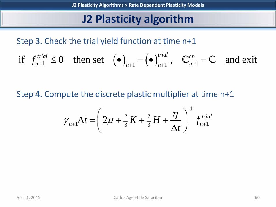
Step 3. Check the trial yield function at time n+1 Step 4. Compute the discrete plastic multiplier at time n+1
J2 Plasticity Algorithms > Rate Dependent Plasticity Models
J2 Plasticity algorithm
April 1, 2015 Carlos Agelet de Saracibar 60
( ) ( )1 11 1if 0 then set , and exittrialtrial ep
n nn nf + ++ +
≤ • = • =
12 2
1 13 32 trialn nt K H f
tηγ µ
−
+ + ∆ = + + + ∆

Step 5. Return mapping algorithm (closest-point-projection)
J2 Plasticity Algorithms > Rate Dependent Plasticity Models
J2 Plasticity algorithm
April 1, 2015 Carlos Agelet de Saracibar 61
( )1
1 1 1 1trialn
trial trialn n n nt fγ
++ + + += − ∆ ∂
SS S C S
12 2
1 1 1 13 3
12 2
1 1 13 3
12 2
1 1 1 13 3
2 2
: 2 2 3
2: 23
trial trial trialn n n n
trial trialn n n
trial trial trialn n n n
K H ft
q q K H f Kt
K H f Ht
ηµ µ
ηµ
ηµ
−
+ + + +
−
+ + +
−
+ + + +
= − + + + ∆ = − + + + ∆ = + + + + ∆
σ σ n
q q n

Step 6. Update plastic internal variables database at time n+1
J2 Plasticity Algorithms > Rate Dependent Plasticity Models
J2 Plasticity algorithm
April 1, 2015 Carlos Agelet de Saracibar 62
( )1
1 1 1trialn
p p trialn n n nt fγ
++ + += + ∆ ∂
SE E S
12 2
1 1 13 3
12 2
1 13 3
12 2
1 1 13 3
2
2 2 3
2
p p trial trialn n n n
trialn n n
trial trialn n n n
K H ft
K H ft
K H ft
ηµ
ηξ ξ µ
ηµ
−
+ + +
−
+ +
−
+ + +
= + + + + ∆ = + + + + ∆ = − + + + ∆
ε ε n
ξ ξ n
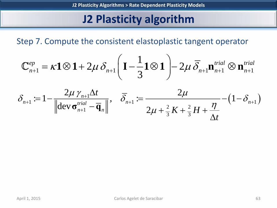
Step 7. Compute the consistent elastoplastic tangent operator
J2 Plasticity Algorithms > Rate Dependent Plasticity Models
J2 Plasticity algorithm
April 1, 2015 Carlos Agelet de Saracibar 63
1 1 1 1 112 23
ep trial trialn n n n nκ µδ µδ+ + + + +
= ⊗ + − ⊗ − ⊗
1 1 I 1 1 n n
( )11 1 1
2 213 3
2 2: 1 , : 1dev 2
nn n ntrial
n n
t
K Ht
µ γ µδ δ δηµ
++ + +
+
∆= − = − −
− + + +∆
σ q

Nonlinear isotropic hardening Exponential saturation law + linear hardening
J2 Plasticity Algorithms > Rate Dependent Plasticity Models
Nonlinear isotropic hardening
April 1, 2015 Carlos Agelet de Saracibar 64
( ) ( ):q ξ ξψ ξ ξ′= −∂ = −∂ Π = −Π
( ) ( )( ): : 1 expYq Kξψ σ σ δξ ξ∞= −∂ = − − − − −
( ) ( ) ( )( )1 expY Kξ σ σ δξ ξ∞′Π = − − − +
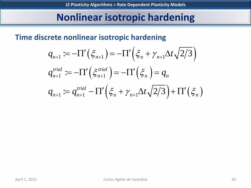
Time discrete nonlinear isotropic hardening
J2 Plasticity Algorithms > Rate Dependent Plasticity Models
Nonlinear isotropic hardening
April 1, 2015 Carlos Agelet de Saracibar 65
( ) ( )( ) ( )
( ) ( )
1 1 1
1 1
1 1 1
: 2 3
:
: 2 3
n n n n
trial trialn n n n
trialn n n n n
q t
q q
q q t
ξ ξ γ
ξ ξ
ξ γ ξ
+ + +
+ +
+ + +
′ ′= −Π = −Π + ∆
′ ′= −Π = −Π =
′ ′= −Π + ∆ +Π
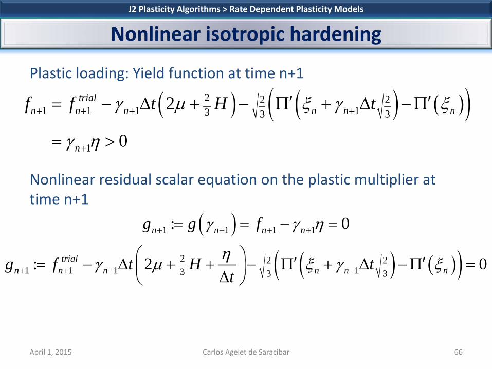
Plastic loading: Yield function at time n+1
Nonlinear residual scalar equation on the plastic multiplier at time n+1
J2 Plasticity Algorithms > Rate Dependent Plasticity Models
Nonlinear isotropic hardening
April 1, 2015 Carlos Agelet de Saracibar 66
( ) ( ) ( )( )2 2 21 1 1 13 3 3
1
2
0
trialn n n n n n
n
f f t H tγ µ ξ γ ξ
γ η
+ + + +
+
′ ′= − ∆ + − Π + ∆ −Π
= >
( )
( ) ( )( )1 1 1 1
2 2 21 1 1 13 3 3
: 0
: 2 0
n n n n
trialn n n n n n
g g f
g f t H tt
γ γ η
ηγ µ ξ γ ξ
+ + + +
+ + + +
= = − =
′ ′= − ∆ + + − Π + ∆ −Π = ∆

Newton-Raphson iterative solution algorithm Step 1. Initialize iteration counter and plastic multiplier Step 2. Compute the residual g at time n+1, iteration k Step 3. While the absolute value of the current residual at time n+1, iteration k, is greater than a tolerance Step 4. Solve the linarized equation Step 5. Update the plastic multiplier at time n+1, iteration k+1 Step 6. Compute the residual g at time n+1, iteration k+1 Step 7. Increment iteration counter k=k+1 and go to Step 3
J2 Plasticity Algorithms > Rate Dependent Plasticity Models
Nonlinear isotropic hardening
April 1, 2015 Carlos Agelet de Saracibar 67
10, 0knk γ += =
1 1 1 0k k kn n ng Dg γ+ + ++ ∆ =
11 1 1
k k kn n nγ γ γ++ + += + ∆

Newton-Raphson iterative solution algorithm
J2 Plasticity Algorithms > Rate Dependent Plasticity Models
Nonlinear isotropic hardening
April 1, 2015 Carlos Agelet de Saracibar 68
( ) ( )( )( )
( )
21 1 1 3
2 213 3
2 2 21 1 1 1 13 3 3
2 221 13 33
: 2
: 2
: 2
k trial kn n n
kn n n
k k k k kn n n n n n
k kn n n
g f t Ht
t
Dg H t t tt
t H tt
ηγ µ
ξ γ ξ
ηγ µ γ ξ γ γ
ηµ ξ γ γ
+ + +
+
+ + + + +
+ +
= − ∆ + + ∆
′ ′− Π + ∆ −Π
′′∆ = − + + ∆ ∆ − Π + ∆ ∆ ∆ ∆ ′′= − + Π + ∆ + + ∆ ∆ ∆
1 1 1 0k k kn n ng Dg γ+ + ++ ∆ =
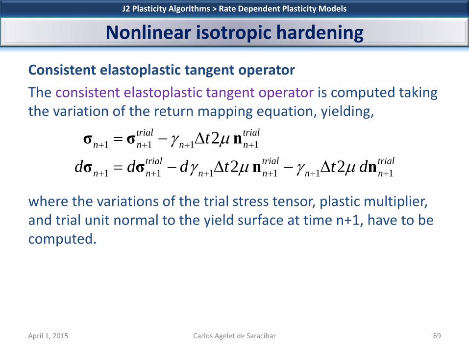
Consistent elastoplastic tangent operator The consistent elastoplastic tangent operator is computed taking the variation of the return mapping equation, yielding, where the variations of the trial stress tensor, plastic multiplier, and trial unit normal to the yield surface at time n+1, have to be computed.
J2 Plasticity Algorithms > Rate Dependent Plasticity Models
Nonlinear isotropic hardening
April 1, 2015 Carlos Agelet de Saracibar 69
1 1 1 1
1 1 1 1 1 1
2
2 2
trial trialn n n n
trial trial trialn n n n n n
td d d t t d
γ µ
γ µ γ µ+ + + +
+ + + + + +
= − ∆
= − ∆ − ∆
σ σ nσ σ n n

The variation of the plastic multiplier at time n+1 is computed setting the variation of the residual at time n+1 equal to zero,
J2 Plasticity Algorithms > Rate Dependent Plasticity Models
Nonlinear isotropic hardening
April 1, 2015 Carlos Agelet de Saracibar 70
( ) ( )( )( )
( )
2 2 21 1 1 13 3 3
2 2 21 1 1 1 13 3 3
2 221 1 13 33
21 3
: 2 0
: 2
: 2 0
2
trialn n n n n n
trialn n n n n n
trialn n n n
n n
g f t H tt
dg df d t H t d tt
df d t t Ht
d t
ηγ µ ξ γ ξ
ηγ µ ξ γ γ
ηγ µ ξ γ
γ µ ξ
+ + + +
+ + + + +
+ + +
+
′ ′= − ∆ + + − Π + ∆ −Π = ∆ ′′= − ∆ + + − Π + ∆ ∆ ∆ ′′= − ∆ + Π + ∆ + + = ∆
′′∆ = + Π +( )1
221 133
trialn nt H df
tηγ
−
+ + ∆ + + ∆

Substituting the variations shown before, the following discrete tangent constitutive equation can be obtained, where the consistent elastoplastic tangent operator at time n+1 is given by
and the following parameters have been introduced
J2 Plasticity Algorithms > Rate Dependent Plasticity Models
Nonlinear isotropic hardening
April 1, 2015 Carlos Agelet de Saracibar 71
1 1 1:epn n nd d+ + +=σ ε
1 1 1 1 112 23
ep trial trialn n n n nκ µδ µδ+ + + + +
= ⊗ + − ⊗ − ⊗
1 1 I 1 1 n n
( )( )1
1 1 12 221
13 33
2 2: 1 , : 1dev 2
nn n ntrial
n nn n
t
t Ht
µ γ µδ δ δηµ ξ γ
++ + +
++
∆= − = − −
− ′′+ Π + ∆ + +∆
σ q

Contents 1. Introduction 2. J2 Rate independent plasticity models
1. Return mapping algorithm 2. Consistent elastoplastic tangent modulus 3. Step by step algorithm 4. Nonlinear isotropic hardening
3. J2 Rate dependent plasticity models 1. Return mapping algorithm 2. Consistent elastoplastic tangent modulus 3. Step by step algorithm 4. Nonlinear isotropic hardening
4. J2 Computational plasticity assignment
J2 Plasticity Algorithms > Contents
Contents
April 1, 2015 Carlos Agelet de Saracibar 72

Implement in MATLAB the BE time-stepping algorithm for J2 rate-independent/rate-dependent hardening plasticity models, including linear and nonlinear isotropic hardening, and linear kinematic hardening
Perform the numerical simulation of uniaxial cyclic plastic loading/elastic unloading examples for the following cases: o Rate-independent/rate-dependent perfect plasticity o Rate-independent/rate-dependent linear isotropic hardening plasticity o Rate-independent/rate-dependent nonlinear isotropic hardening
plasticity, considering an exponential saturation law o Rate-independent/rate-dependent linear kinematic hardening
plasticity o Rate-independent/rate-dependent nonlinear isotropic and linear
kinematic hardening plasticity
J2 Plasticity Algorithms > J2 Computational Plasticity Assignment
J2 Computational plasticity assignment
April 1, 2015 Carlos Agelet de Saracibar 73
For the perfect plasticity models, plot the stress11-strain11 and the dev[stress11]-strain11 curves.
For the linear isotropic/linear kinematic hardening models, plot the stress11-strain11 and dev[stress11]-strain11 curves showing the influence of the isotropic/kinematic hardening parameters
For the nonlinear isotropic hardening model, plot the stress11-strain11 and dev[stress11]-strain11 curves showing the influence of the exponential coefficient of the exponential saturation law
J2 Plasticity Algorithms > J2 Computational Plasticity Assignment
J2 Computational plasticity assignment
April 1, 2015 Carlos Agelet de Saracibar 74

For the rate-dependent plasticity models, plot the stress11-strain11, dev[stress11]-strain11, and the stress11-time and dev[stress11]-time curves showing the influence of the viscosity parameter and the loading rate.
Show that the rate-independent response can be recovered from the rate-dependent results using very small values for the viscosity or the loading rate
J2 Plasticity Algorithms > J2 Computational Plasticity Assignment
J2 Computational plasticity assignment
April 1, 2015 Carlos Agelet de Saracibar 75

Write a comprehensive deliverable report (10 pages) providing the data of the cyclic loading and material properties considered, the stress-strain curves, and the stress-time curves for the rate-dependent plasticity examples. Add suitable comments on the results, comparing the influence of the different material parameters and loading conditions.
Add a printed copy of the subroutines as an Appendix
J2 Plasticity Algorithms > J2 Computational Plasticity Assignment
J2 Computational plasticity assignment
April 1, 2015 Carlos Agelet de Saracibar 76