Chapter 4. Improving Triangulations with Curvature ...lori/dissertation/Ch4.pdf · MS(p i,j) =...

Chapter 4.

Improving Triangulations with Curvature

Equalization

Both hierarchical triangulations described in chapter 3 can produce excel-

lent surface approximations, given the right initial triangulation. Yet a poor initial

triangulation can throw these methods off, introducing artifacts that persist

through all levels of detail. For example, the triangulation may contain more tri-

angles than are needed, which would increase storage space and time required to

render the surface. It may also contain too many slivery triangles — characterized

by at least one very acute angle — which cause artifacts in the display and anom-

alies in some analysis functions like finite element analysis. Refinement tech-

niques often introduce artifacts at the coarser levels of detail because critical fea-

tures are not always evident at those levels. Instead, several refinement iterations

are required before these features are revealed. The work described here solves

this problem of finding a good initial triangulation.

70 Spatial Data Representations

4.1. Foundations

Intuitively speaking, a good triangulation will approximate a surface with

a few large triangles over smooth areas, and many small triangles over rough

areas. I hypothesize that this may be achieved by equalizing the curvature under

each triangle.

Consider, for example, the triangulation of a paraboloid which has equal

curvature everywhere. The best triangulation is achieved with a mesh of triangles

with equal area; the placement of the vertices is unimportant. This is demonstrat-

ed by showing that for an equilateral triangle approximating the surface of the

paraboloid — with each vertex on the surface of the paraboloid — the point of

greatest error is in the center of the triangle, regardless of where the triangle is.

Furthermore, the error at that point is h2/3, where h is the length of each side of

the equilateral triangle.

To check the consistency of this idea with the strategy of my adaptive

hierarchical triangulation, I re-ran adaptive hierarchical triangulation on the eight

test cases described earlier and measured the curvature of triangles that required

refinement versus those that didn't. On average, triangles requiring refinement

had curvature values three times greater than those that didn't.

Then question then is how to equalize the curvatures in a triangulated

model of a surface? This section provides some of the background for my search

for an answer.

Improving Triangulations with Curvature Equalization 71

4.1.1. Polygonal curve approximations

An analogy to this problem may be found in the one-dimensional case

where a curve is approximated with a series of straight line segments, as shown in

figure 4.1. Starting with a line segment connecting the two endpoints of the curve

(a), an approximation may be produced by successively splitting line segments at

points of greatest error (b) until the line segments fit the curve within a given tol-

erance (c). Although the resulting approximation is error-free, it contains more

points than necessary. In the one-dimensional case, this problem is solved by

merging line segments (d). As shown, the two middle segments are merged so

that the curvature of each interval represented by a line segment is roughly the

same. Pavlidis’ text [Pav77] describes this split-and-merge technique in detail.

The literature on polygonal approximations is extensive [Pav77, McC75,

SK76, Mon70, T74, DH73]. Some of these methods are based on the result that in

an optimal polygonal approximation vertices are placed so that an integral of the

curvature takes the same value over all intervals [McC75]. In contrast, the litera-

ture on triangulated approximations is comparatively limited [MS88, Nad86,

DLR90]. Extending polygonal approximation techniques to triangulations is diffi-

cult because there is no direct counterpart of merging triangles for the two-dimen-

sional case.


(a) (b) (c) (d)

Figure 4.1. Improving linear approximations with a slit-and-merge technique

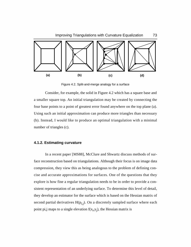
Consider, for example, the solid in Figure 4.2 which has a square base and

a smaller square top. An initial triangulation may be created by connecting the

four base points to a point of greatest error found anywhere on the top plane (a).

Using such an initial approximation can produce more triangles than necessary

(b). Instead, I would like to produce an optimal triangulation with a minimal

number of triangles (c).

4.1.2. Estimating curvature

In a recent paper [MS88], McClure and Shwartz discuss methods of sur-

face reconstruction based on triangulations. Although their focus is on image data

compression, they view this as being analogous to the problem of defining con-

cise and accurate approximations for surfaces. One of the questions that they

explore is how fine a regular triangulation needs to be in order to provide a con-

sistent representation of an underlying surface. To determine this level of detail,

they develop an estimator for the surface which is based on the Hessian matrix of

second partial derivatives H(pi,j). On a discretely sampled surface where each

point pi,j maps to a single elevation f(xi,yj), the Hessian matrix is


(a) (b) (c) (d)

Figure 4.2. Split-and-merge analogy for a surface

H(pi,j) = [ fxx fxy ]fxy fyy

For each point pi,j the curvature estimator is expressed by

MS(pi,j) = 3(trace H(pi,j))2 - 8(det H(pi,j))

= 3(fxx2 + 2fxxfyy + fyy

2) - 8(fxxfyy - fxy2)

= 2fxx2. + 2fyy

2 + (fxx - fyy)2 + 8fxy2

which is always a positive value.

There are several ways of generating this Hessian matrix. The second par-

tial derivatives of pi,j may be approximated as follows:

fxx = f(xi-1,yj) + f(xi+1,yj) - 2f(xi,yj)

fyy = f(xi,yj-1) + f(xi,yj+1) - 2f(xi,yj)

fxy = fyx = f(xi-1,yj-1) + f(xi+1,yj+1) - f(xi-1,yj+1) - f(xi+1,yj-1).

For continuous or irregularly sampled data, these second partial deriva-

tives can come directly from the quadratic equation for the curvature at that point,

expressed as

ax2 + bxy + cy2 + dx + ey + f = z.

This equation may be found

through Gaussian elimination (if five

nearest neighbors are used) or least

squares approximation (if more neigh-

bors are used).

Although this curvature esti-

mator is not curvature in the classical

sense, I use the term loosely because

this measure detects the salient fea-


x

y

Figure 4.3. Gaussian curvature alone will

not detect all critical features, such as this

edge of a cliff

tures of a surface. In fact, the above measure incorporates both the mean curva-

ture (approximated by the trace of the Hessian) and the Gaussian curvature

(approximated by the determinant of the Hessian). This improves on simpler

measures such as the determinant of the Hessian which fail to detect many critical

features in real-world situations. Consider, for example, the edge of a cliff as

shown in Figure 4.3. Although points along this edge are clearly critical to the

model, the determinant of the Hessian at these points is zero.

With this curvature estimate for each point on the surface, the curvature of

a triangle can be expressed as an integral of this measure over the entire triangle.

When the surface is represented by a set of discrete sample points, the curvature

of a triangle may be approximated by summing these measures for all points

within it.

In their extensions section of [MS88], McClure and Shwartz discuss how

this estimator relates to the selection of nonhomogeneous (irregular) triangles for

approximating the surface. Although they provide an expression for the ideal den-

sity of distributed sample points and triangles, they do not give an actual algo-

rithm for selecting these points and triangles.

4.2. Approach

My approach is to extend the ideas of polygonal approximation to a high-

er dimension. Since it is not feasible to extend the split-and-merge algorithm to

triangulations, I follow the alternative strategy of moving vertices. I move these

vertices — and collapse very thin pairs of triangles — so that the triangles

approximate surface patches of similar curvature.


Curvature equalization starts with a triangulation that covers the surface

with the required level of granularity, but is not optimal. It may, for example, con-

tain more triangles than are needed and/or too many slivery triangles. I assume

that the triangulation corresponds to a known underlying surface or bivariate

function which is sampled at regular intervals, such as a digital terrain model.

Error in the triangulation is measured by projecting each of these sample points to

the appropriate triangle, then taking the difference between the actual and project-

ed values. The triangulation meets error constraints if none of these errors

exceeds a given tolerance value.

I attempt to improve the model by moving triangle vertices so that curva-

tures associated with the triangles are as nearly equivalent as possible. This must

be done without introducing errors to the model. The curvature of each triangle is

approximated by summing the curvature estimates for all sample points (as

described above) within a triangle. Points coincident with triangle edges are not

included in these sums. Indeed the goal of the algorithm is to place such bound-

aries over areas of high curvature, keeping triangle interiors relatively flat.

I use a three-step procedure for moving vertices. The first step shifts trian-

gle vertices, attempting to equalize curvatures within the triangles. The second

step collapses unnecessary triangles, further reducing the number of triangles in

the model. The third step switches edge directions across pairs of triangles to

reduce sliveriness without introducing errors. All three algorithms are described

in greater detail below.


4.2.1. Initial Triangulation

Because the purpose of this algorithm is to improve existing triangula-

tions, one must first provide the initial triangulation. For gridded surface models,

the initial triangulation is simply generated for a subsampled set of points.

For sparse irregular surface models, such as those provided by Michigan

State University [LS91], care must be taken that the initial triangulation only cov-

ers valid data areas. To accomplish this, I first find the convex hull of the data.

This is used to generate the α-shape of the data set [Ede87]1 with an operator-

specified α. A set of interior points that have high curvature are also selected for

the triangulation. To ensure that these interior points are evenly distributed over

the surface, the surface is partitioned into subregions. One point of highest curva-

ture in then selected in each subregion. The MSU data also requires an adaptive

grid for the surface as described in chapter 3. Once these points have been found,

the results are triangulated with an inward spiral TIN generation algorithm

[McK87].

For full three-dimensional data, the initial triangulation may be generated

from a subsampling of the model produced using Hoppe et al.’s surface recon-

struction algorithm [HDDMS91]. This algorithm finds neighborhoods and sur-

face tangents for each data point, which are used to approximate curvature and

generate a regular initial triangulation. Once point-triangle relationships have

been established, any triangulation may be processed by curvature equalization.


1. The α-shape captures the general shape of a set of points, separating “foreground” from “back-ground”. The parameter α determines the level of detail captured in this shape.

4.2.2. Equalizing curvature

The algorithm of the first step

attempts to equalize curvature by itera-

tively reducing the size of the triangles

with greatest curvature. This size

reduction is achieved by moving each vertex of the triangle inward, one at a time.

A vertex may conceivably move anywhere within the triangle, although prefer-

ence is given to points of highest curvature. This movement is further restricted to

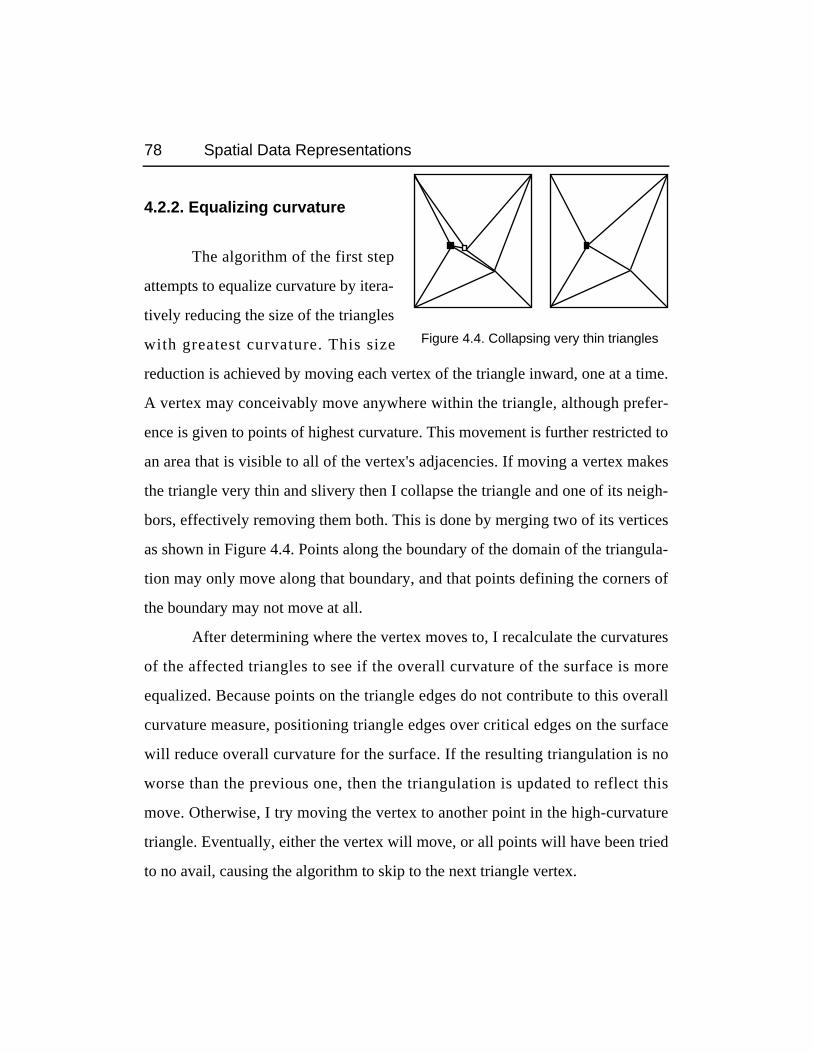
an area that is visible to all of the vertex's adjacencies. If moving a vertex makes

the triangle very thin and slivery then I collapse the triangle and one of its neigh-

bors, effectively removing them both. This is done by merging two of its vertices

as shown in Figure 4.4. Points along the boundary of the domain of the triangula-

tion may only move along that boundary, and that points defining the corners of

the boundary may not move at all.

After determining where the vertex moves to, I recalculate the curvatures

of the affected triangles to see if the overall curvature of the surface is more

equalized. Because points on the triangle edges do not contribute to this overall

curvature measure, positioning triangle edges over critical edges on the surface

will reduce overall curvature for the surface. If the resulting triangulation is no

worse than the previous one, then the triangulation is updated to reflect this

move. Otherwise, I try moving the vertex to another point in the high-curvature

triangle. Eventually, either the vertex will move, or all points will have been tried

to no avail, causing the algorithm to skip to the next triangle vertex.


Figure 4.4. Collapsing very thin triangles

There are several reasons why triangle

curvatures may never be completely equal. One

factor is the discrete nature of the data. Vertices

may only move to known points on the underly-

ing surface. Another factor is the finite bounds

on the triangulated area. Consider, for example,

the ridge in Figure 4.5, indicated by the dark line.

Because points of high curvature occur only

along this ridge, curvature cannot be equalized in

any triangulation in which this ridge corresponds

to a triangle edge. To prevent cycling — moving a vertex back and forth between

two points on the surface — I keep a record of all attempted moves. Any move

that has been tried before is automatically rejected, and the algorithm proceeds to

the next vertex. If no vertices may move in the triangle of highest curvature, the

pointer is incremented to a new triangle with maximum curvature.

Curvature equalization continues to try moving vertices until the triangle

with “maximum” curvature has curvature equal to the smallest curvature in the

triangulation. If it is unable to move any vertices on the triangle of highest curva-

ture, it proceeds to the triangle of next-highest curvature and considers that as the

triangle of “maximum” curvature. Because the algorithm skips over triangles in

this manner — and doesn’t allow repeated moves — either the curvature within

the triangulation will become equal, or the “maximum” triangle will eventually

be the same as the “minimum”, and the algorithm will halt.

This algorithm for this first step is summarized in the pseudo-code of fig-

ure 4.6.


High

High

Low

Low

Figure 4.5. Curvature of a sur-

face model cannot always be

truly equalized


procedure equalize_curvatures (Point, Triangle, Member, Point_Curvature,

Triangle_Curvature )

Input : An initial triangulation Triangle that references a Point set defining

the surface, with a Point_Curvature measure and 0..2 triangle

Members for each p ∈ Point , and a summed Triangle_Curvature

for each t ∈Triangle.

Output : Updated Triangle, Triangle_Curvature , and Members .

begin

sort triangles on Triangle_Curvature in descending order;

max_tri = triangle at head of the sorted list;

min_tri = triangle at tail of the sorted list;

while Triangle_Curvature[max_tri] >Triangle_Curvature[min_tri] do begin

for each current vertex vi of Triangle[max_tri] do begin

generate queue, in order of descending Point_Curvature,

of all points p such that Triangle[max_tri] ∈ Members[p]

and p is visible from all points adjacent to vi ;

repeat

get candidate vertex point p from queue;

calculate new Triangle_Curvature values if vi moves to p ;

until new triangulation is better or queue is empty;

if new triangulation is better then begin (* update triangulation *)

remove triangles that are too skinny;

split neighbors of skinny triangles as necessary;

update variables: Triangle, Triangle_Curvature , Members ;

update sorted list of triangles;

max_tri = triangle at head of the sorted list;

end;

else if no vertices of Triangle[max_tri] could move then

max_tri = next triangle on sorted list;

end;

end;

end;

Figure 4.6. Algorithm for equalizing curvature

4.2.3. Remove unnecessary triangles

T h e s e c o n d s t e p f u r t h e r

improves the triangulation by removing

unnecessary pairs of triangles. For

example, a planar patch bounded by a

rectangle may be accurately approxi-

mated by several triangles with equal

curvature, as shown in Figure 4.7 (indi-

cated by the lighter lines). However,

only two triangles are actually needed

(represented by the darker lines).

The second step in curvature equalization remedies this by attempting to

remove unnecessary pairs of triangles. Because triangle areas will increase, cur-

vature may also increase. It is more important to examine the actual planar equa-

tions: it is only desirable to merge surface patches that approximate parts of the

same plane.

Two triangles are removed from the triangulation by collapsing their com-

mon edge into a single point as shown in Figure 4.4. It tries to remove every pair

of triangles within the triangulation, resulting in less than 3/2T iterations, where T

is the number of triangles initially. Because an edge may be collapsed into either

of its endpoints, the algorithm tries merging both ways and chooses the better

way.

This algorithm for the second step is summarized in figure 4.8.


Figure 4.7. Triangulations with equalized

curvature may still contain more surface

patches than are necessary

4.2.4. Switch edges

The third step improves the

triangulation by switching the

direction of an edge that splits the

quadrilateral formed by two adja-

cent triangles. As shown in Figure

4.9, this switch from (a) to (b) can

reduce sliveriness.

This step can also reduce error in the model. Although the previous steps

allow vertices to move around and even collapse onto one another, they do not

change the adjacency relationships among the vertices. As observed earlier, if the


a b

Figure 4.9. Motivation for switching edge

directions: slivery triangles (a) can be made

less slivery (b)

procedure remove_unnecessary_triangles (Point, Triangle, Triangle_Curvature )






begin

for each pair of triangles ti ,tj ∈Triangle that share edge pq do

if ti and tj are co-planar then begin

try moving point p to point q ;

try moving point q to point p ;

select the better move to make;

if this does not adversely affect neighboring triangles then

update triangulation;

end;

end;

Figure 4.8. Algorithm for eliminating unnecessary triangles

initial triangulation contains an edge that crosses the model surface the wrong

way, the previous two steps will not be able to remedy this problem. For example,

a triangulation of a ridge — where points and edges were selected without regard

to topographic features — could contain edges that cut across the ridge rather

than follow it. As shown in a recent paper by Southard [So91], this is a common

problem which may be solved more directly by allowing the adjacencies to

change. The triangle conditioning described in this paper inspired my algorithm

for the third step.

My approach is to consider all pairs of triangles that have opposing obtuse

angles. The algorithm switches the direction of the dividing edge if making such

a switch produces less slivery triangles and introduces no additional error. This

algorithm is summarized in figure 4.10.


procedure switch_edges (Point, Triangle, Member, Point_Curvature, Triangle_Curvature

)






begin

for each pair of triangles ti ,tj ∈Triangle that share edge pq do

if opposing angles i and j are both obtuse then begin

calculate new Triangle_Curvature values for ti ,tjgiven that pq is replaced with a new edge splitting i and j ;

if this triangulation is better then

update triangulation;

end;

end;

Figure 4.10. Algorithm for switching edge directions

4.3. Results

I first ran the three curvature equalization algorithms on simple artificial

surfaces that were pre-triangulated. These surfaces — a ridge, a pyramid, and a

paraboloid — are illustrated in Figure 4.11 along with the results of running my

algorithms on them. In this figure, column A shows the original triangulations.

Column B shows the results after equalizing curvature in the first step of my pro-

cedure. Column C shows the results after removing unnecessary triangles in the

second step of my proce-

dure. Column D shows the

results after edge-switching.

In these diagrams darkened

lines represent ridges and

highlighted points move in

the next step. As shown, the

three curvature equalization

steps produced optimal tri-

angulations in al l cases,

a l t h o u g h s o m e f i g u r e s

require more of the steps

than others. This demon-

s t ra tes that my methods

work well for curved as well

as polyhedral surfaces.


PYRAMID

PARABOLOID

CBA D

RIDGE

Figure 4.11. Curvature equalization applied to artificial

test cases

4.3.1. Applying curvature equalization to terrain models

Having demonstrated the effectiveness of curvature equalization on artifi-

cial surfaces, I conducted a number of experiments with real terrain data as

described below. In each experiment I consider three factors: numeric accuracy of

the model, number of triangles in the model, and sliveriness of the triangles as

described in previous chapters.

4.3.1.1. Improving Triangulations that Consider Surface Topology

My first experiment was to apply curvature equalization to the levels of

detail produced by my adaptive hierarchical triangulation described in chapter

3.2. Overall, the results were disappointing. Curvature equalization made little or

no improvement to these surface models. This is because the adaptive hierarchi-

cal triangulation accomplishes similar results by considering surface topology. As

mentioned earlier, adaptive hierarchical triangulation typically splits triangles of

high curvature anyway.

The next experiment was to use curvature equalization to simply improve

the initial triangulation for the adaptive hierarchical triangulation. I hypothesized

that such an initial triangulation would produce better, more consistent hierarchi-

cal triangulations.

To test my hypothesis I used the same eight test areas used to test adaptive

hierarchical triangulation. These represent a variety of terrain types, from flat

plains to rolling hills to jagged mountains. I generated three initial triangulations

for each of the test areas. The first initial triangulation simply split the square area


of interest (AOI) in half along

the diagonal. The second ini-

tial triangulation found the

point farthest from the surface

of a bilinear patch defined by

the four AOI corners, and

split the area into four trian-

gles meeting at that point. The

third initial triangulation was

created by applying curvature

equalization to a regular trian-

gulation with 16 triangles.

I then ran adapt ive

hierarchical triangulation on

the 24 initial triangulations,

producing 5 levels of detail

with an error tolerance of 10

meters at the highest level of

detai l . Tables 4.1 and 4.2

show my results with the best

results shown in bold face for

each tes t case . Table 4 .1

shows the average sliveriness

over all levels of detail in the


Table 4.2. Effects of initial triangulation on number

of triangles in finest level of detail

Split Bilinear CurvatureAOI in Half Split Equalized

1 1852 1852 1834

2 2330 2260 2282

3 1353 1285 1308

4 1123 1015 953

5 3072 3100 2990

6 1998 2096 1933

7 2745 2701 2643

8 4418 4489 4390

Split Bilinear CurvatureAOI in Half Split Equalized

1 5.086 5.087 2.871

2 9.645 9.543 3.202

3 5.934 4.646 2.971

4 11.315 5.497 3.408

5 14.843 10.576 3.432

6 5.305 7.691 3.028

7 4.352 4.921 3.407

8 5.949 6.958 3.060

Table 4.1. Effects of initial triangulation on sliveri-

ness

model, where sliveriness has been normalized so that an equilateral triangle has a

value of 1. In all cases the curvature equalized initial triangulation produced the

least slivery results. Table 4.2 shows the number of triangles in the highest level

of detail. In most cases the curvature equalized initial triangulation required fewer

triangles to achieve the specified level of accuracy, although the differences are

almost negligible in this case.

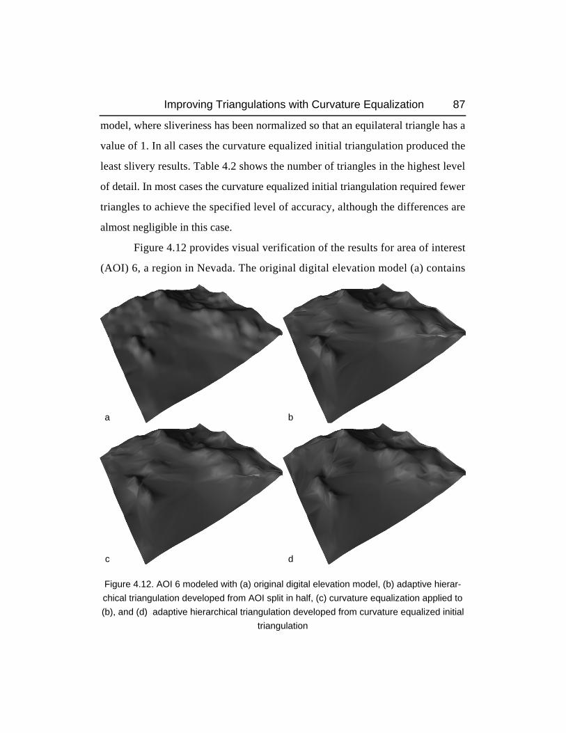
Figure 4.12 provides visual verification of the results for area of interest

(AOI) 6, a region in Nevada. The original digital elevation model (a) contains


Figure 4.12. AOI 6 modeled with (a) original digital elevation model, (b) adaptive hierar-

chical triangulation developed from AOI split in half, (c) curvature equalization applied to

(b), and (d) adaptive hierarchical triangulation developed from curvature equalized initial

triangulation

a b

c d

10,952 triangles. The highest level of detail from an adaptive hierarchical triangu-

lation that initially split the area in half (b) contains 1979 triangles. Here an artifi-

cial ridge imposed by the initial triangulation is clearly visible in the right corner.

Applying curvature equalization to this final level of detail (c) smoothed over this

ridge somewhat. Yet the best results are the 1933 triangles produced from an ini-

tial triangulation that was curvature equalized (d).

Figure 4.13 shows similar results when applied to AOI 1, a region in

Alabama (a). Notice how the severe artifact introduced by the initial half-split (b)


Figure 4.13. AOI 1 modeled with (a) original digital elevation model, (b) adaptive hierar-

chical triangulation developed from AOI split in half, and (c) adaptive hierarchical triangu-

lation developed from curvature equalized initial triangulation

a

b c

is nowhere evident in the model produced from a curvature-equalized initial tri-

angulation (c).

4.3.1.2. Improving Triangulations that Disregard Surface Topology

In my next experiment I explored the results of applying curvature equal-

ization to regular triangulations. Many real- and near-real-time applications such

as flight simulators reduce the number of triangles by producing coarser triangu-

lations from a subsampled grid. Although this has the advantage of simplicity,

vertices selected this way are not necessarily important topologically. Likewise,

discarded points are not necessarily unimportant. I hypothesized that curvature

equalization could improve these regular triangulations.


Subsampled Every 9th Point Subsampled Every 4th PointCurvature Equalization Reduces Curvature Equalization Reduces

AOI # of Triangles Error # of Triangles Error

1 32.0% 12.4% 21.9% 0.7%

2 32.0% 7.0% 2.8% 5.3%

3 63.3% 22.7% 7.4% 5.1%

4 44.5% 9.0% 38.1% 3.1%

5 17.2% 10.3% 15.1% 2.8%

6 43.0% 6.5% 4.2% 10.3%

7 44.5% 0.0% 0.3% 0.3%

8 41.4% 21.5% 19.9% 0.0%

Table 4.3. Effects of equalizing curvature of subsampled digital elevation models

I used the same eight AOIs mentioned previously to test my hypothesis.

Table 4.3 shows the results of equalizing curvature of triangulations produced

from two subsamplings. Taking every 4th point reduced each model from 10,952

to 648 triangles. Likewise, taking every 9th point reduced the model to 128 trian-

gles. The columns in the table show, in both cases, how curvature equalization

was able to further reduce both the number of triangles and numeric error in the

model. Results are more significant for the larger subsampling rate because spars-

er samples are more likely to miss the critical features of the surface.


Figure 4.14. AOI 1 modeled with (a) original digital elevation model,

(b) subsampled regular grid, and (c) curvature equalized subsampled grid

a

b c

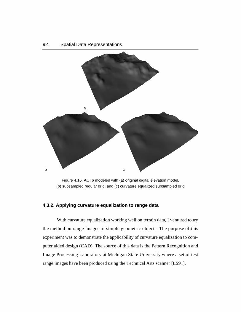
Figures 4.14 through 4.16 show the results of curvature equalization in

three cases. Each figure shows a) the original data, b) the data subsampled at

every fourth point, and c) the result of applying curvature equalization to the sub-

sampled model. Figure 4.14 shows the effects of this on AOI 1 where curvature

equalization reduced the number of triangles by 21.9% and the error by 0.7%.

Figure 4.15 shows AOI 2 where curvature equalization reduced the number of tri-

angles by 2.8% and the error by 5.3%. Figure 4.16 shows AOI 6 where curvature

equalization reduced the number of triangles by 4.2% and the error by 10.3%.




a

b c

4.3.2. Applying curvature equalization to range data

With curvature equalization working well on terrain data, I ventured to try

the method on range images of simple geometric objects. The purpose of this

experiment was to demonstrate the applicability of curvature equalization to com-

puter aided design (CAD). The source of this data is the Pattern Recognition and

Image Processing Laboratory at Michigan State University where a set of test

range images have been produced using the Technical Arts scanner [LS91].




a

b c

Differences between this range data and the terrain data are numerous.

First, the range data represent points scattered over the surface. Large areas where

the data is invalid (i.e. not on the object surface) are blank. This necessitates the

use of an artificial grid to organize the data, as described in section 3.2, and a tri-

angulation of the α-shape of the data, as mentioned in 4.2. The second difference

is the data type. The floating point values of the range data introduce precision

errors that were not evident with the integer elevation values. To overcome this

problem, I've re-introduced the idea of nearness used in the adaptive hierarchical

triangulation: a point near an edge is treated as if it is on the edge. A point is con-

sidered near an edge if the edge passes through the grid cell containing that point.

Yet the greatest difference of all is between the surfaces represented.

Terrain generally forms a continuous surface with few sharp discontinuities.

Hence the approximations described earlier for the second partial derivatives pro-

duce reasonable values for calculating the Gaussian and mean curvature at each

point. Geometric objects, on the other hand, are often characterized by sharp dis-

continuities. Because curvature is not defined on such edges, common estimation

methods are prone to error.

I ran curvature equalization on three of these geometric objects with dis-

appointing results. Although the algorithm did equalize curvature, it did not move

the vertices to critical points and edges to critical lines on the surface as I had

expected. The desired results were finally achieved by first running adaptive hier-

archical triangulation on the initial triangulation to add vertices and edges at the

critical junctures. Even then several iterations of the three curvature equalization

steps were required before the optimal solution was achieved.


Closer inspection revealed that unexpect-

ed curvature values are the culprit. On a square-

based pyramid with ridges along the diagonals,

points on the ridges have greater curvature values

than the peak. Yet if the pyramid is rotated 45˚

about the z axis, the peak will have the greatest

curvature value. This phenomenon is illustrated in figure 4.17 which shows two

windows over a ridge of height h. Using the simple estimate of the second partial

derivatives described earlier, the trace of the Hessian matrix is -2h for the window

on the left and -4h for the window on the right. This indicates that large errors are

creeping into the mean curvature which is supposed to be rotation invariant.

The trouble lies with the estimation of the second partial derivatives.

Unlike terrain, the pyramid has sharp discontinuities that foul up this estimator.

Using numerical differentiation — adding correction terms using data beyond the

immediate locale of a point [DB74] — reduces the difference in the trace values,

but does not eliminate it.

Naturally I was disappointed that the extension to a new data type did not

work immediately. Yet I have not yet exhausted the realm of possibilities for cur-

vature equalization. Chapter 7 lists future extensions to this work which, I

believe, will render it applicable to the geometric data typical to computer aided

design (CAD).


0 h 0 h 0 00 h 0 0 h 0

0 h 0 0 0 h

Figure 4.17. Window over a

ridge of height h at two different

orientations

Chapter 4. Improving Triangulations with Curvature ...lori/dissertation/Ch4.pdf · MS(p i,j) =...

Documents

Transcript of Chapter 4. Improving Triangulations with Curvature ...lori/dissertation/Ch4.pdf · MS(p i,j) =...