Chapter 4 IMAGE PROCESSINGnceg.uop.edu.pk/workshop-17to31mar-05/Slides/Day2... · Chapter 4 IMAGE...
88
Workshop/Training on “Earthquake Vulnerability and Multi- Hazard Risk Assessment: Geospatial Tools for Rehabilitation and Reconstruction Efforts” held at National Centre of Excellence in Geology, Peshawar, Pakistan from 13 to 31 March 2006 Ch4-p87 Associated Institute Chapter 4 IMAGE PROCESSING ILWIS for Windows contains a set of image processing tools for enhancement and analysis of data from space borne or airborne platforms. In this chapter, the routine applications such as image enhancement, classification and geo- referencing are described. The image enhancement techniques, explained in this chapter, make it possible to modify the appearance of images for optimum visual interpretation. Spectral classification of remotely sensed data is related to computer-assisted interpretation of these data. Geo-referencing remote sensed data refers to geometric distortions, the relationship between an image and a coordinate system, the transformation function and resampling techniques. Remotely sensed data Remotely sensed data, such as satellite images, are measurements of reflected solar radiation, energy emitted by the earth itself or energy emitted by Radar systems that is reflected by the earth. An image consists of an array of pixels (picture elements) or grid cells which are ordered in rows and columns. Each pixel has a digital number (DN) that represents the intensity of the received signal reflected or emitted by a given area of the earth surface. The size of the area belonging to a pixel is called the spatial resolution. The DN is produced in a sensor-system dependent range, the radiometric values. An image may consist of many layers or bands. Each band is created by the sensor that collects energy in specific wavelengths of the electro-magnetic spectrum. Before you can start with the exercises, you should start up ILWIS and change to the working subdirectory c:\EVMHRAGTRRE\Chapter4, where the data files for this chapter are stored. • Double-click the ILWIS program icon. • Change the working drive and the working directory until you are in the directory c:\EVMHRAGTRRE\Chapter4.
Transcript of Chapter 4 IMAGE PROCESSINGnceg.uop.edu.pk/workshop-17to31mar-05/Slides/Day2... · Chapter 4 IMAGE...
Workshop/Training on “Earthquake Vulnerability and Multi- Hazard Risk Assessment: Geospatial Tools for Rehabilitation and Reconstruction Efforts” held at National Centre of Excellence in Geology, Peshawar, Pakistan from 13 to 31 March 2006
Ch4-p87
Associated Institute
Chapter 4 IMAGE PROCESSING
ILWIS for Windows contains a set of image processing tools for enhancement and analysis of data from space borne or airborne platforms. In this chapter, the routine applications such as image enhancement, classification and geo-referencing are described. The image enhancement techniques, explained in this chapter, make it possible to modify the appearance of images for optimum visual interpretation. Spectral classification of remotely sensed data is related to computer-assisted interpretation of these data. Geo-referencing remote sensed data refers to geometric distortions, the relationship between an image and a coordinate system, the transformation function and resampling techniques.
Remotely sensed data Remotely sensed data, such as satellite images, are measurements of reflected solar radiation, energy emitted by the earth itself or energy emitted by Radar systems that is reflected by the earth. An image consists of an array of pixels (picture elements) or grid cells which are ordered in rows and columns. Each pixel has a digital number (DN) that represents the intensity of the received signal reflected or emitted by a given area of the earth surface. The size of the area belonging to a pixel is called the spatial resolution. The DN is produced in a sensor-system dependent range, the radiometric values. An image may consist of many layers or bands. Each band is created by the sensor that collects energy in specific wavelengths of the electro-magnetic spectrum.
Before you can start with the exercises, you should start up ILWIS and change to the working subdirectory c:\EVMHRAGTRRE\Chapter4, where the data files for this chapter are stored.
• Double-click the ILWIS program icon. • Change the working drive and the working directory until you are
in the directory c:\EVMHRAGTRRE\Chapter4.
Workshop/Training on “Earthquake Vulnerability and Multi- Hazard Risk Assessment: Geospatial Tools for Rehabilitation and Reconstruction Efforts” held at National Centre of Excellence in Geology, Peshawar, Pakistan from 13 to 31 March 2006
Ch4-p88
Associated Institute
3.1 Visualization of images
Single band images For satellite images and scanned black and white aerial photographs the image domain is used. Pixels in a satellite image or scanned aerial photograph usually have values ranging from 0-255. The values of the pixels represent the reflectance of the surface object. The image domain is in fact a special case of a value domain. Raster maps using the image domain are stored using the ‘1 byte’ per pixel storage format. A single band image can be visualized in terms of its gray shades, ranging from black (0) to white (255). To compare bands or to compare image bands before and after an operation, the images can be displayed in different windows, visible on the screen at the same time. The relationship between gray shades and pixel values can also be detected. The pixel location in an image (rows and columns), can be linked to a georeference which in turn is linked to a coordinate system which can have a defined map projection. In this case, the coordinates of each pixel in the window are displayed if one points to it. The objectives of the exercises in this section are:
- to understand the relationship between the digital numbers of satellite images and the display, and
- to be able to display several images, scroll through and zoom in/out on the images and retrieve the digital numbers of the displayed images.
Satellite or airborne digital image data is composed of a two-dimensional array of discrete picture elements or pixels. The intensity of each pixel corresponds to the average brightness, or radiance, measured electronically over the ground area corresponding to each pixel. Remotely sensed data can be displayed by reading the file from disk line-by-line and writing the output to a monitor. Typically, the Digital Numbers (DNs) in a digital image are recorded over a numerical range of 0 to 255 (8 bits = 28 = 256), although some images have other numerical ranges, such as, 0 to 63 (4 bits = 24 = 64), or 0 to 1023 (10 bits = 210 = 1024). The display unit has usually a display depth of 8 bits. Hence, it can display images in 256 (gray) tones. The following Landsat 7 path 150 Row 036 ETM+ (Enhanced Thematic Mapper plus) bands of Northeastern Pakistan are of 2001 October 07 having 30m spatial resolution for multispectral and 15 for panchromatic are used in this exercise (thermal band is resampled from 60 meters to 30 meters):
ETM+band 1 : etmb1 ETM+band 4 : etmb4 ETM+band 6L: etmb6a ETM+band 3 : etmb3 ETM+band 5 : etmb5 ETM+band 6H: etmb6b ETM+band 7 : etmb7 ETM+pan : etmpan

Workshop/Training on “Earthquake Vulnerability and Multi- Hazard Risk Assessment: Geospatial Tools for Rehabilitation and Reconstruction Efforts” held at National Centre of Excellence in Geology, Peshawar, Pakistan from 13 to 31 March 2006
Ch4-p89
Associated Institute
About Landsat7 ETM+:
At launch, the satellite will weigh about 4,800 lbs (2,200 kg) and is about 14 ft long (4.3 m) and 9 ft (2.8 m) in diameter. The satellite will be placed in a circular orbit at 438 miles (705 km) above the earth. As the students are cutting out the paper model, describe the various components of the Landsat-7 satellite. Key components include:
ETM+ (Enhanced Thematic Mapper Plus) instrument package. The ETM+ will acquire data in the visible, near infrared, middle infrared, and thermal bands. The spatial resolution is 49 ft (15 m)
in the panchromatic band (the pan band covers a wide band of wavelengths, similar to standard black-and-white aerial photographs), 98 ft (30 m) in the visible, near infrared and middle infrared wavelengths, and 197 ft (60 m) in the thermal infrared band. ETM+ will image the earth in a 115-mile (185Km) wide swath. The computer running the ETM+ receives instructions from the mission ground control folks. The computer translates these instructions and tells the ETM+ when to turn on and off to take the images.
The X-band antenna. The X-band antenna is used to receive instructions from the mission control folks on the ground. Daily commands are sent to the Landsat-7 spacecraft telling the ETM+ what images to record and when to downlink the image data, either to U.S. or international ground stations.
Solar array. A solar array is a collection of solar panels that work together to collect energy from the sun and is used to power the Landsat-7 satellite.
Launch of the Landsat-7 satellite was from the Western Test Range at Vandenberg Air Force Base, CA, on a Delta-II Expendable Launch Vehicle. The launch occurred on 15 April 1999.
See additional information about Landsat-7 in the Background section (http://ltpwww.gsfc.nasa.gov/landsat7/teacherkit/html/ls7background.html). Fact sheet about Landsat-7: http://pao.gsfc.nasa.gov/gsfc/service/gallery/fact_sheets/earthsci/landsat7.htm Source: http://ltpwww.gsfc.nasa.gov/landsat7/teacherkit/html/ls7overview.html
Landsat7 Orbit Characteristics
Altitude 705 km
Inclination 98.2 degree
Period 98.9 minute Recurrent period 16 days equatorial crossing time 10:00 am Swath Width 185 km
Landsat 7 and ETM+ Characteristics
Band Number
Spectral Range(microns)
Ground Resolution(m)
1 .45 to .515 30
2 .525 to .605 30
3 .63 to .690 30
4 .75 to .90 30
5 1.55 to 1.75 30
6 10.40 to 12.5 60
7 2.09 to 2.35 30
Pan .52 to .90 15
Workshop/Training on “Earthquake Vulnerability and Multi- Hazard Risk Assessment: Geospatial Tools for Rehabilitation and Reconstruction Efforts” held at National Centre of Excellence in Geology, Peshawar, Pakistan from 13 to 31 March 2006
Ch4-p90
Associated Institute
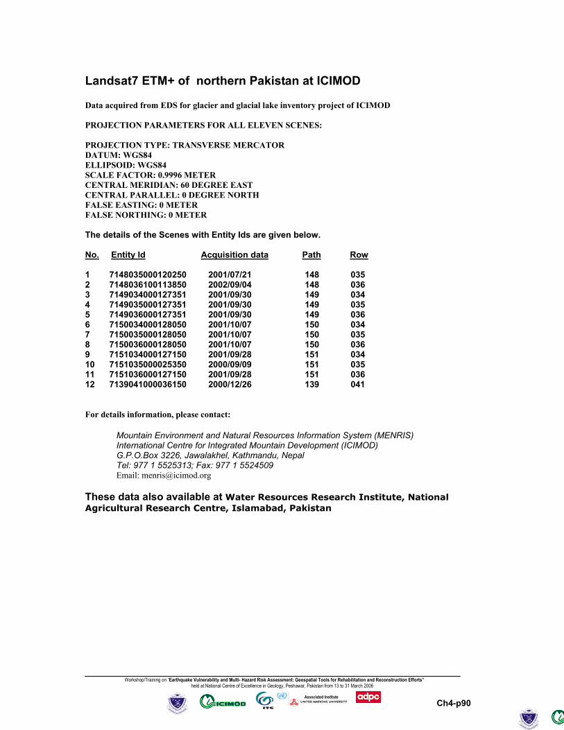
Landsat7 ETM+ of northern Pakistan at ICIMOD Data acquired from EDS for glacier and glacial lake inventory project of ICIMOD PROJECTION PARAMETERS FOR ALL ELEVEN SCENES: PROJECTION TYPE: TRANSVERSE MERCATOR DATUM: WGS84 ELLIPSOID: WGS84 SCALE FACTOR: 0.9996 METER CENTRAL MERIDIAN: 60 DEGREE EAST CENTRAL PARALLEL: 0 DEGREE NORTH FALSE EASTING: 0 METER FALSE NORTHING: 0 METER The details of the Scenes with Entity Ids are given below. No. Entity Id Acquisition data Path Row 1 7148035000120250 2001/07/21 148 035 2 7148036100113850 2002/09/04 148 036 3 7149034000127351 2001/09/30 149 034 4 7149035000127351 2001/09/30 149 035 5 7149036000127351 2001/09/30 149 036 6 7150034000128050 2001/10/07 150 034 7 7150035000128050 2001/10/07 150 035 8 7150036000128050 2001/10/07 150 036 9 7151034000127150 2001/09/28 151 034 10 7151035000025350 2000/09/09 151 035 11 7151036000127150 2001/09/28 151 036 12 7139041000036150 2000/12/26 139 041 For details information, please contact:
Mountain Environment and Natural Resources Information System (MENRIS) International Centre for Integrated Mountain Development (ICIMOD) G.P.O.Box 3226, Jawalakhel, Kathmandu, Nepal Tel: 977 1 5525313; Fax: 977 1 5524509 Email: [email protected]
These data also available at Water Resources Research Institute, National Agricultural Research Centre, Islamabad, Pakistan
Workshop/Training on “Earthquake Vulnerability and Multi- Hazard Risk Assessment: Geospatial Tools for Rehabilitation and Reconstruction Efforts” held at National Centre of Excellence in Geology, Peshawar, Pakistan from 13 to 31 March 2006
Ch4-p91
Associated Institute
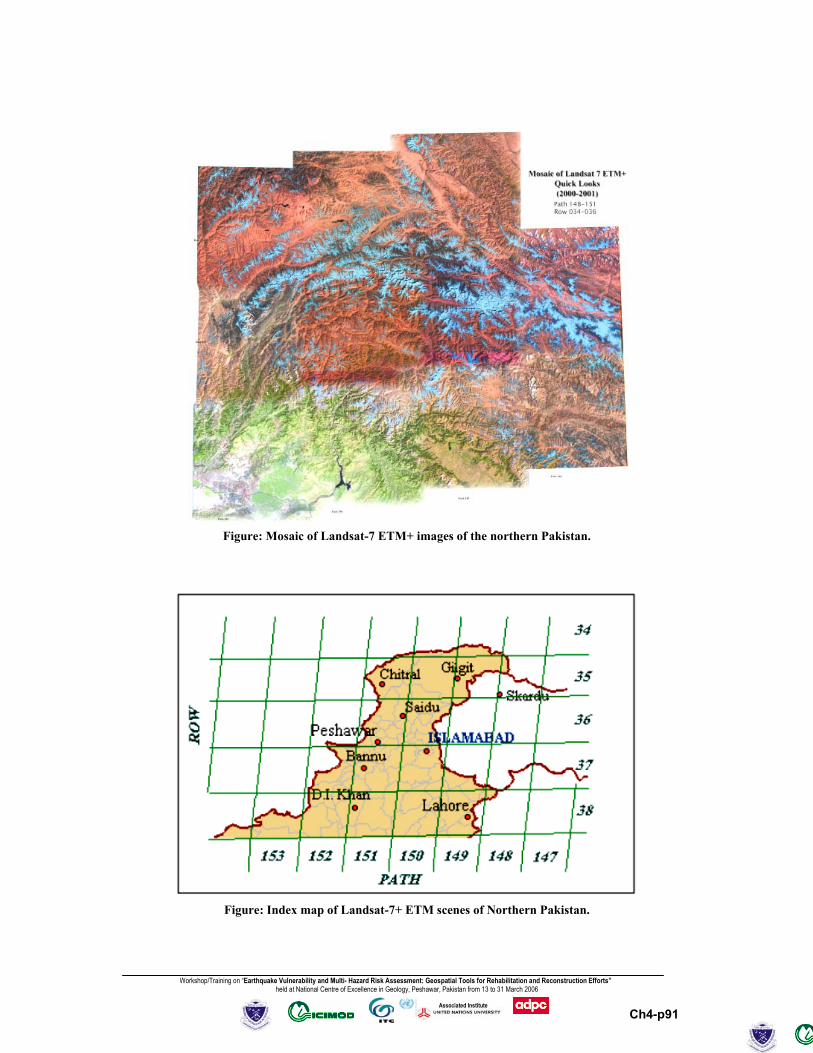
Figure: Mosaic of Landsat-7 ETM+ images of the northern Pakistan.
Figure: Index map of Landsat-7+ ETM scenes of Northern Pakistan.
Workshop/Training on “Earthquake Vulnerability and Multi- Hazard Risk Assessment: Geospatial Tools for Rehabilitation and Reconstruction Efforts” held at National Centre of Excellence in Geology, Peshawar, Pakistan from 13 to 31 March 2006
Ch4-p92
Associated Institute
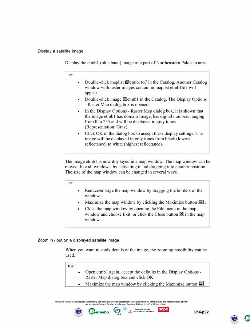
Display a satellite image
Display the etmb1 (blue band) image of a part of Northeastern Pakistan area.
• Double-click maplist etmb1to7 in the Catalog. Another Catalog window with raster images contain in maplist etmb1to7 will appear.
• Double-click image etmb1 in the Catalog. The Display Options - Raster Map dialog box is opened.
• In the Display Options - Raster Map dialog box, it is shown that the image etmb1 has domain Image, has digital numbers ranging from 0 to 255 and will be displayed in gray tones (Representation: Gray).
• Click OK in the dialog box to accept these display settings. The image will be displayed in gray tones from black (lowest reflectance) to white (highest reflectance).
The image etmb1 is now displayed in a map window. The map window can be moved, like all windows, by activating it and dragging it to another position. The size of the map window can be changed in several ways.
• Reduce/enlarge the map window by dragging the borders of the
window. • Maximize the map window by clicking the Maximize button . • Close the map window by opening the File menu in the map
window and choose Exit, or click the Close button in the map window.
Zoom in / out on a displayed satellite image
When you want to study details of the image, the zooming possibility can be used.
• Open etmb1 again, accept the defaults in the Display Options -
Raster Map dialog box and click OK. • Maximize the map window by clicking the Maximize button
Workshop/Training on “Earthquake Vulnerability and Multi- Hazard Risk Assessment: Geospatial Tools for Rehabilitation and Reconstruction Efforts” held at National Centre of Excellence in Geology, Peshawar, Pakistan from 13 to 31 March 2006
Ch4-p93
Associated Institute
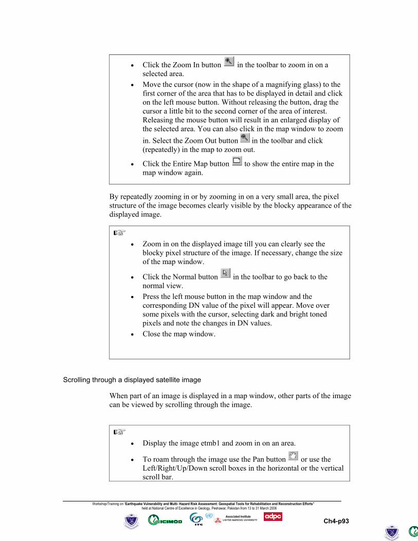
• Click the Zoom In button in the toolbar to zoom in on a selected area.
• Move the cursor (now in the shape of a magnifying glass) to the first corner of the area that has to be displayed in detail and click on the left mouse button. Without releasing the button, drag the cursor a little bit to the second corner of the area of interest. Releasing the mouse button will result in an enlarged display of the selected area. You can also click in the map window to zoom in. Select the Zoom Out button in the toolbar and click (repeatedly) in the map to zoom out.
• Click the Entire Map button to show the entire map in the map window again.
By repeatedly zooming in or by zooming in on a very small area, the pixel structure of the image becomes clearly visible by the blocky appearance of the displayed image.
• Zoom in on the displayed image till you can clearly see the
blocky pixel structure of the image. If necessary, change the size of the map window.
• Click the Normal button in the toolbar to go back to the normal view.
• Press the left mouse button in the map window and the corresponding DN value of the pixel will appear. Move over some pixels with the cursor, selecting dark and bright toned pixels and note the changes in DN values.
• Close the map window.
Scrolling through a displayed satellite image
When part of an image is displayed in a map window, other parts of the image can be viewed by scrolling through the image.
• Display the image etmb1 and zoom in on an area.
• To roam through the image use the Pan button or use the Left/Right/Up/Down scroll boxes in the horizontal or the vertical scroll bar.
Workshop/Training on “Earthquake Vulnerability and Multi- Hazard Risk Assessment: Geospatial Tools for Rehabilitation and Reconstruction Efforts” held at National Centre of Excellence in Geology, Peshawar, Pakistan from 13 to 31 March 2006
Ch4-p94
Associated Institute
• A fast scroll can also be achieved by dragging the scroll boxes in the scroll bars Left/Right or Up/Down, or by clicking in the scroll bar itself.
• Close the map window.
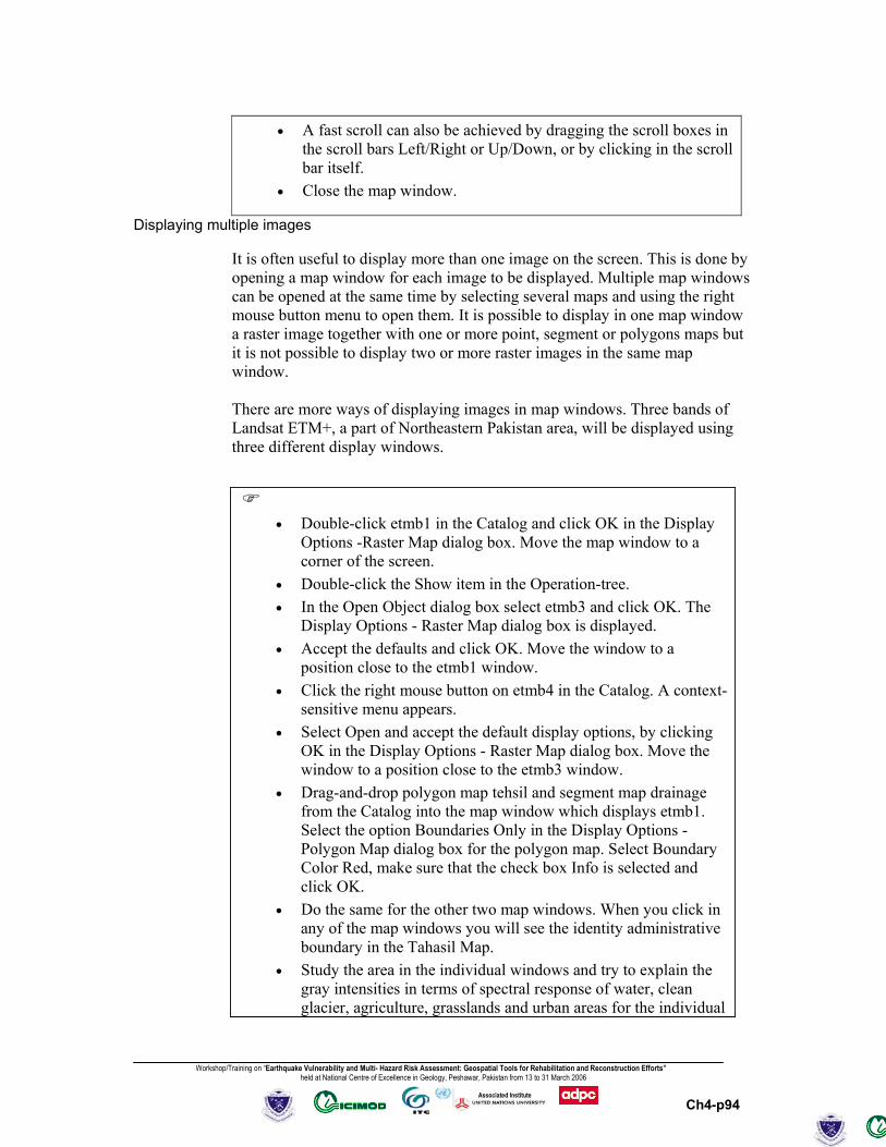
Displaying multiple images
It is often useful to display more than one image on the screen. This is done by opening a map window for each image to be displayed. Multiple map windows can be opened at the same time by selecting several maps and using the right mouse button menu to open them. It is possible to display in one map window a raster image together with one or more point, segment or polygons maps but it is not possible to display two or more raster images in the same map window. There are more ways of displaying images in map windows. Three bands of Landsat ETM+, a part of Northeastern Pakistan area, will be displayed using three different display windows.
• Double-click etmb1 in the Catalog and click OK in the Display
Options -Raster Map dialog box. Move the map window to a corner of the screen.
• Double-click the Show item in the Operation-tree. • In the Open Object dialog box select etmb3 and click OK. The
Display Options - Raster Map dialog box is displayed. • Accept the defaults and click OK. Move the window to a
position close to the etmb1 window. • Click the right mouse button on etmb4 in the Catalog. A context-
sensitive menu appears. • Select Open and accept the default display options, by clicking
OK in the Display Options - Raster Map dialog box. Move the window to a position close to the etmb3 window.
• Drag-and-drop polygon map tehsil and segment map drainage from the Catalog into the map window which displays etmb1. Select the option Boundaries Only in the Display Options - Polygon Map dialog box for the polygon map. Select Boundary Color Red, make sure that the check box Info is selected and click OK.
• Do the same for the other two map windows. When you click in any of the map windows you will see the identity administrative boundary in the Tahasil Map.
• Study the area in the individual windows and try to explain the gray intensities in terms of spectral response of water, clean glacier, agriculture, grasslands and urban areas for the individual

Workshop/Training on “Earthquake Vulnerability and Multi- Hazard Risk Assessment: Geospatial Tools for Rehabilitation and Reconstruction Efforts” held at National Centre of Excellence in Geology, Peshawar, Pakistan from 13 to 31 March 2006
Ch4-p95
Associated Institute
bands. Write down the relative spectral response as ‘low’, ‘medium’ or ‘high’, for the different land cover classes and spectral bands in Table below.
• Close all map windows after you have finished the exercise.
Table : Relative spectral responses per band for different land cover classes. Fill in the table with classes: low, medium and high
Band Water Clean glacier Agriculture Grass land Urban area 1 2 3 4 5 6a 6b 7
Digital numbers and pixels The spectral responses of the earth’s surface in specific wavelengths, recorded by the spectrometers on board of a satellite, are assigned to picture elements (pixels). Pixels with a strong spectral response have high digital numbers and vise versa. The spectral response of objects can change over the wavelengths recorded, as you have seen in the exercise comparing different Landsat ETM+ bands with regard to water and clean glacier areas. When a gray scale is used, pixels with a weak spectral response are dark toned (black) and pixels representing a strong spectral response are bright toned (white). The digital numbers are thus represented by intensities on a black to white scale. The digital numbers themselves can be retrieved through a pixel information window. This window offers the possibility to inspect interactively and simultaneously, the pixel values in one or more images. There are several ways to open and add maps to the pixel information window.
• Display map etmb1 in a map window. • From the File menu in the map window, select Open Pixel
Information. The pixel information window appears. • Make sure that the pixel information window can be seen on the
screen. Select etmb3 and etmb4 in the Catalog and drag these maps to the pixel information window: hold the left mouse button down; move the mouse pointer to the pixel information window; and release the left mouse button; The images are dropped in the pixel information window.

Workshop/Training on “Earthquake Vulnerability and Multi- Hazard Risk Assessment: Geospatial Tools for Rehabilitation and Reconstruction Efforts” held at National Centre of Excellence in Geology, Peshawar, Pakistan from 13 to 31 March 2006
Ch4-p96
Associated Institute
• Display etmb4, click OK in the Display Options - Raster Map dialog box. Make sure that the map window does not overlap with the pixel information window.
• In the pixel information window the DNs of all three selected bands will be displayed. Zoom in if necessary.
You can also add maps one by one to the pixel information window (File menu Add Map). Roam through image etmb4 and write down in Table below some DN values for water, Clean glacier area, agriculture, scrubs and grassland. For ground truth, topographic map of area can be used.
Table: DN values of different land cover classes of selected spectral bands. Fill in
the DN values yourself
Band Water Clean glacier Agriculture Grass land Urban area 1 2 3 4 5 6a 6b 7
• Close the pixel information window.
It is also possible to use the Command line of the Main window to add multiple maps to a pixel information window.
• Type on the Command line of the Main window: Pixelinfo
etmb1.mpr etmb3.mpr etmb4.mpr. The pixel information window opens and contains the maps etmb1, etmb3 and etmb4.
• Close all windows after finishing the exercise.
Pixels and real world coordinates When an image is created, either by a satellite, airborne scanner or by an office scanner, the image is stored in row and column geometry in raster format. There is no relationship between the rows/columns and real world coordinates
Workshop/Training on “Earthquake Vulnerability and Multi- Hazard Risk Assessment: Geospatial Tools for Rehabilitation and Reconstruction Efforts” held at National Centre of Excellence in Geology, Peshawar, Pakistan from 13 to 31 March 2006
Ch4-p97
Associated Institute
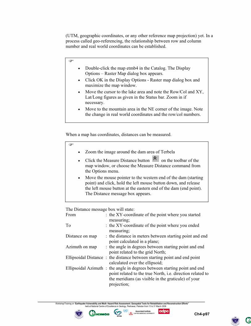
(UTM, geographic coordinates, or any other reference map projection) yet. In a process called geo-referencing, the relationship between row and column number and real world coordinates can be established.
• Double-click the map etmb4 in the Catalog. The Display
Options – Raster Map dialog box appears. • Click OK in the Display Options - Raster map dialog box and
maximize the map window. • Move the cursor to the lake area and note the Row/Col and XY,
Lat/Long figures as given in the Status bar. Zoom in if necessary.
• Move to the mountain area in the NE corner of the image. Note the change in real world coordinates and the row/col numbers.
When a map has coordinates, distances can be measured.
• Zoom the image around the dam area of Terbela
• Click the Measure Distance button on the toolbar of the map window, or choose the Measure Distance command from the Options menu.
• Move the mouse pointer to the western end of the dam (starting point) and click, hold the left mouse button down, and release the left mouse button at the eastern end of the dam (end point). The Distance message box appears.
The Distance message box will state: From : the XY-coordinate of the point where you started
measuring; To : the XY-coordinate of the point where you ended
measuring; Distance on map : the distance in meters between starting point and end
point calculated in a plane; Azimuth on map : the angle in degrees between starting point and end
point related to the grid North; Ellipsoidal Distance : the distance between starting point and end point
calculated over the ellipsoid; Ellipsoidal Azimuth : the angle in degrees between starting point and end
point related to the true North, i.e. direction related to the meridians (as visible in the graticule) of your projection;
Workshop/Training on “Earthquake Vulnerability and Multi- Hazard Risk Assessment: Geospatial Tools for Rehabilitation and Reconstruction Efforts” held at National Centre of Excellence in Geology, Peshawar, Pakistan from 13 to 31 March 2006
Ch4-p98
Associated Institute
Scale Factor : direct indicator of scale distortion, i.e. the ratio between distance on the map / true distance.
• Click OK in the Distance message box. • Close the map window after finishing the exercise.
Summary: Visualization of images
- Satellite or airborne digital images are composed of a two-dimensional array
of discrete picture elements or pixels. The intensity of each pixel corresponds to the average brightness, or radiance, measured electronically over the ground area corresponding to each pixel.
- A single band image can be visualized in terms of its gray shades, ranging
from black (0) to white (255).
- Pixels with a weak spectral response are dark toned (black) and pixels
representing a strong spectral response are bright toned (white). The digital numbers are thus represented by intensities from black to white.
- To compare bands and understand the relationship between the digital
numbers of satellite images and the display, and to be able to display several images, you can scroll through and zoom in/out on the images and retrieve the DNs of the displayed images.
- In one map window, a raster image can be displayed together with point,
segment or polygon maps. It is not possible in ILWIS to display two raster maps in one map window.
- An image is stored in row and column geometry in raster format. When you
obtain an image there is no relationship between the rows/columns and real world coordinates (UTM, geographic coordinates, or any other reference map projection) yet. In a process called geo-referencing, the relationship between row and column number and real world coordinates can be established.
Workshop/Training on “Earthquake Vulnerability and Multi- Hazard Risk Assessment: Geospatial Tools for Rehabilitation and Reconstruction Efforts” held at National Centre of Excellence in Geology, Peshawar, Pakistan from 13 to 31 March 2006
Ch4-p99
Associated Institute
3.2 Image enhancements
Image enhancement deals with the procedures of making a raw image better interpretable for a particular application. In this section, commonly used enhancement techniques are described, which improve the visual impact of the raw remotely sensed data for the human eye. Image enhancement techniques can be classified in many ways. Contrast enhancement, also called global enhancement, transforms the raw data using the statistics computed over the whole data set. Examples are: linear contrast stretch, histogram equalized stretch and piece-wise contrast stretch. Contrary to this, spatial or local enhancement only take local conditions into consideration and these can vary considerably over an image. Examples are image smoothing and sharpening.
3.2.1 Contrast enhancement
The objective of this section is to understand the concept of contrast enhancement and to be able to apply commonly used contrast enhancement techniques to improve the visual interpretation of an image. The sensitivity of the on-board sensors of satellites, has been designed in such a way that they record a wide range of brightness characteristics, under a wide range of illumination conditions. Few individual scenes show a brightness range that fully utilizes the brightness range of the detectors. The goal of contrast enhancement is to improve the visual interpretability of an image, by increasing the apparent distinction between the features in the scene. Although the human mind is excellent in distinguishing and interpreting spatial features in an image, the eye is rather poor at discriminating the subtle differences in reflectance that characterize such features. By using contrast enhancement techniques these slight differences are amplified to make them readily observable. Contrast stretch is also used to minimize the effect of haze. Scattered light that reaches the sensor directly from the atmosphere, without having interacted with objects at the earth surface, is called haze or path radiance. Haze results in overall higher DN values and this additive effect results in a reduction of the contrast in an image. The haze effect is different for the spectral ranges recorded; highest in the blue, and lowest in the infrared range of the electromagnetic spectrum. Techniques used for contrast enhancement are: the linear stretching technique and the histogram equalization. To enhance specific data ranges showing certain land cover types the piece-wise linear contrast stretch can be applied. A computer monitor on which the satellite imagery is displayed is capable of displaying 256 gray levels (0 - 255). This corresponds with the resolution of most satellite images, as their digital numbers also vary within the range of 0 to 255. To produce an image of optimal contrast, it is important to utilize the full brightness range (from black to white through a variety of gray tones) of the display medium.
Workshop/Training on “Earthquake Vulnerability and Multi- Hazard Risk Assessment: Geospatial Tools for Rehabilitation and Reconstruction Efforts” held at National Centre of Excellence in Geology, Peshawar, Pakistan from 13 to 31 March 2006
Ch4-p100
Associated Institute
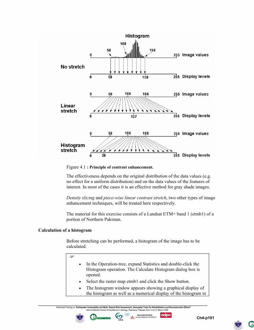
The linear stretch (Figure 4.1) is the simplest contrast enhancement. A DN value in the low end of the original histogram is assigned to extreme black, and a value at the high end is assigned to extreme white. The remaining pixel values are distributed linearly between these extremes. One drawback of the linear stretch is that it assigns as many display levels to the rarely occurring DN values as it does to the frequently occurring values. A complete linear contrast stretch where (min, max) is stretched to (0, 255) produces in most cases a rather dull image. Even though all gray shades of the display are utilized, the bulk of the pixels is displayed in mid gray. This is caused by the more or less normal distribution, with the minimum and maximum values in the tail of the distribution. For this reason it is common to cut off the tails of the distribution at the lower and upper range. The histogram equalization technique (Figure 4.1) is a non-linear stretch. In this method, the DN values are redistributed on the basis of their frequency. More different gray tones are assigned to the frequently occurring DN values of the histogram. Figure 4.1 shows the principle of contrast enhancement. Assume an output device capable of displaying 256 gray levels. The histogram shows digital values in the limited range of 58 to 158. If these image values were directly displayed, only a small portion of the full possible range of display levels would be used. Display levels 0 to 57 and 159 to 255 are not utilized. Using a linear stretch, the range of image values (58 to 158) would be expanded to the full range of display levels (0 to 255). In the case of linear stretch, the bulk of the data (between 108 and 158) are confined to half the output display levels. In a histogram equalization stretch, the image value range of 108 to 158 is now stretched over a large portion of the display levels (39 to 255). A smaller portion (0 to 38) is reserved for the less numerous image values of 58 to 108.
Workshop/Training on “Earthquake Vulnerability and Multi- Hazard Risk Assessment: Geospatial Tools for Rehabilitation and Reconstruction Efforts” held at National Centre of Excellence in Geology, Peshawar, Pakistan from 13 to 31 March 2006
Ch4-p101
Associated Institute
Figure 4.1 : Principle of contrast enhancement. The effectiveness depends on the original distribution of the data values (e.g. no effect for a uniform distribution) and on the data values of the features of interest. In most of the cases it is an effective method for gray shade images. Density slicing and piece-wise linear contrast stretch, two other types of image enhancement techniques, will be treated here respectively. The material for this exercise consists of a Landsat ETM+ band 1 (etmb1) of a portion of Northern Pakistan.
Calculation of a histogram
Before stretching can be performed, a histogram of the image has to be calculated.
• In the Operation-tree, expand Statistics and double-click the Histogram operation. The Calculate Histogram dialog box is opened.
• Select the raster map etmb1 and click the Show button. • The histogram window appears showing a graphical display of
the histogram as well as a numerical display of the histogram in
Workshop/Training on “Earthquake Vulnerability and Multi- Hazard Risk Assessment: Geospatial Tools for Rehabilitation and Reconstruction Efforts” held at National Centre of Excellence in Geology, Peshawar, Pakistan from 13 to 31 March 2006
Ch4-p102
Associated Institute
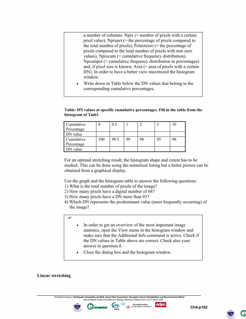
a number of columns: Npix (= number of pixels with a certain pixel value), Npixpct (= the percentage of pixels compared to the total number of pixels), Pctnotzero (= the percentage of pixels compared to the total number of pixels with non zero values), Npixcum (= cumulative frequency distribution), Npcumpct (= cumulative frequency distribution in percentages) and, if pixel size is known, Area (= area of pixels with a certain DN). In order to have a better view maximized the histogram window.
• Write down in Table below the DN values that belong to the corresponding cumulative percentages.
Table: DN values at specific cumulative percentages. Fill in the table from the histogram of Tmb1.
Cumulative Percentage
0 0.5 1 2 5 10
DN value Cumulative Percentage
100 99.5 99 98 95 90
DN value For an optimal stretching result, the histogram shape and extent has to be studied. This can be done using the numerical listing but a better picture can be obtained from a graphical display. Use the graph and the histogram table to answer the following questions: 1) What is the total number of pixels of the image? 2) How many pixels have a digital number of 68? 3) How many pixels have a DN more than 93? 4) Which DN represents the predominant value (most frequently occurring) of
the image?
• In order to get an overview of the most important image
statistics, open the View menu in the histogram window and make sure that the Additional Info command is active. Check if the DN values in Table above are correct. Check also your answer to question 4.
• Close the dialog box and the histogram window.
Linear stretching
Workshop/Training on “Earthquake Vulnerability and Multi- Hazard Risk Assessment: Geospatial Tools for Rehabilitation and Reconstruction Efforts” held at National Centre of Excellence in Geology, Peshawar, Pakistan from 13 to 31 March 2006
Ch4-p103
Associated Institute
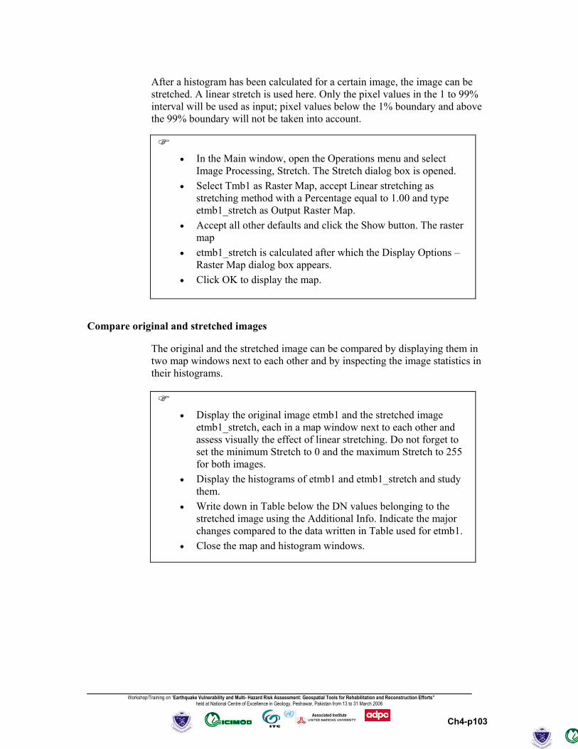
After a histogram has been calculated for a certain image, the image can be stretched. A linear stretch is used here. Only the pixel values in the 1 to 99% interval will be used as input; pixel values below the 1% boundary and above the 99% boundary will not be taken into account.
• In the Main window, open the Operations menu and select Image Processing, Stretch. The Stretch dialog box is opened.
• Select Tmb1 as Raster Map, accept Linear stretching as stretching method with a Percentage equal to 1.00 and type etmb1_stretch as Output Raster Map.
• Accept all other defaults and click the Show button. The raster map
• etmb1_stretch is calculated after which the Display Options – Raster Map dialog box appears.
• Click OK to display the map.
Compare original and stretched images
The original and the stretched image can be compared by displaying them in two map windows next to each other and by inspecting the image statistics in their histograms.
• Display the original image etmb1 and the stretched image
etmb1_stretch, each in a map window next to each other and assess visually the effect of linear stretching. Do not forget to set the minimum Stretch to 0 and the maximum Stretch to 255 for both images.
• Display the histograms of etmb1 and etmb1_stretch and study them.
• Write down in Table below the DN values belonging to the stretched image using the Additional Info. Indicate the major changes compared to the data written in Table used for etmb1.
• Close the map and histogram windows.
Workshop/Training on “Earthquake Vulnerability and Multi- Hazard Risk Assessment: Geospatial Tools for Rehabilitation and Reconstruction Efforts” held at National Centre of Excellence in Geology, Peshawar, Pakistan from 13 to 31 March 2006
Ch4-p104
Associated Institute
Table : DN values at specific cumulative percentages. Fill in the table from the histogram of etmb1_stretch.
Cumulative Percentage
0 0.5 1 2 5 10
DN value Cumulative Percentage
100 99.5 99 98 95 90
DN value
Different linear stretch functions
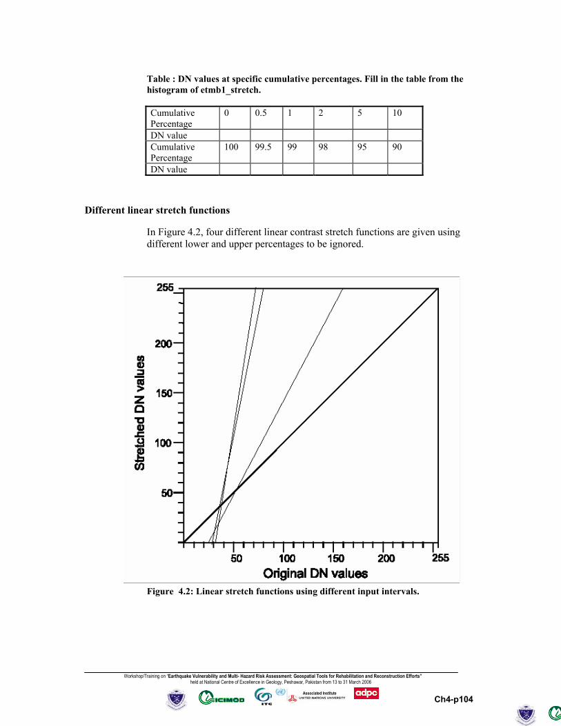
In Figure 4.2, four different linear contrast stretch functions are given using different lower and upper percentages to be ignored.
Figure 4.2: Linear stretch functions using different input intervals.
Workshop/Training on “Earthquake Vulnerability and Multi- Hazard Risk Assessment: Geospatial Tools for Rehabilitation and Reconstruction Efforts” held at National Centre of Excellence in Geology, Peshawar, Pakistan from 13 to 31 March 2006
Ch4-p105
Associated Institute
These four functions were derived using: 1) No stretching 2) Stretching between minimum and maximum values 3) 1 and 99% as lower and upper percentages 4) 5 and 95% as lower and upper percentages [The Landsat7 ETM+ images data provide contain lots of values (33.91%) with zero values which is out of frame of the original Landsat7 ETM+ images. Consider the values with Pctnotzero (= the percentage of pixels compared to the total number of pixels with non zero values]
! Indicate for each line in Figure 4.2, which linear stretch function is shown. Histogram equalization
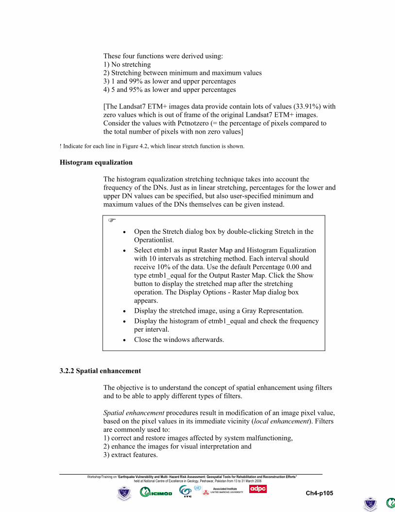
The histogram equalization stretching technique takes into account the frequency of the DNs. Just as in linear stretching, percentages for the lower and upper DN values can be specified, but also user-specified minimum and maximum values of the DNs themselves can be given instead.
• Open the Stretch dialog box by double-clicking Stretch in the Operationlist.
• Select etmb1 as input Raster Map and Histogram Equalization with 10 intervals as stretching method. Each interval should receive 10% of the data. Use the default Percentage 0.00 and type etmb1_equal for the Output Raster Map. Click the Show button to display the stretched map after the stretching operation. The Display Options - Raster Map dialog box appears.
• Display the stretched image, using a Gray Representation. • Display the histogram of etmb1_equal and check the frequency
per interval. • Close the windows afterwards.
3.2.2 Spatial enhancement
The objective is to understand the concept of spatial enhancement using filters and to be able to apply different types of filters. Spatial enhancement procedures result in modification of an image pixel value, based on the pixel values in its immediate vicinity (local enhancement). Filters are commonly used to: 1) correct and restore images affected by system malfunctioning, 2) enhance the images for visual interpretation and 3) extract features.

Workshop/Training on “Earthquake Vulnerability and Multi- Hazard Risk Assessment: Geospatial Tools for Rehabilitation and Reconstruction Efforts” held at National Centre of Excellence in Geology, Peshawar, Pakistan from 13 to 31 March 2006
Ch4-p106
Associated Institute
Like all image enhancement procedures, the objective is to create new images from the original image data, in order to increase the amount of information that can be visually interpreted. Spatial frequency filters, often simply called spatial filters, may emphasize or suppress image data of various spatial frequencies. Spatial frequency refers to the roughness of the variations in DN values occurring in an image. In high spatial frequency areas, the DN values may change abruptly over a relatively small number of pixels (e.g. across roads, field boundaries, shorelines). Smooth image areas are characterized by a low spatial frequency, where DN values only change gradually over a large number of pixels (e.g. large homogeneous ice fields, water bodies). Low pass filters are designed to emphasize low frequency features and to suppress the high frequency component of an image. High pass filters do just the reverse. Low pass filters. Applying a low pass filter has the effect of filtering out the high and medium frequencies and the result is an image, which has a smooth appearance. Hence, this procedure is sometimes called image smoothing and the low pass filter is called a smoothing filter. It is easy to smooth an image. The basic problem is to do this without losing interesting features. For this reason much emphasis in smoothing is on edge-preserving smoothing. High pass filters. Sometimes abrupt changes from an area of uniform DNs to an area with other DNs can be observed. This is represented by a steep gradient in DN values. Boundaries of this kind are known as edges. They occupy only a small area and are thus high-frequency features. High pass filters are designed to emphasize high frequencies and to suppress low-frequencies. Applying a high pass filter has the effect of enhancing edges. Hence, the high pass filter is also called an edge-enhancement filter. Two classes of high-pass filters can be distinguished: gradient (or directional) filters and Laplacian (or non-directional) filters. Gradient filters are directional filters and are used to enhance specific linear trends. They are designed in such a way that edges running in a certain direction (e.g. horizontal, vertical or diagonal) are enhanced. In their simplest form, they look at the difference between the DN of a pixel to its neighbor and they can be seen as the result of taking the first derivative (i.e. the gradient). Laplacian filters are non-directional filters because they enhance linear features in any direction in an image. They do not look at the gradient itself, but at the changes in gradient. In their simplest form, they can be seen as the result of taking the second derivative. A filter usually consists of a 3x3 array (sometimes called kernel) of coefficients or weighting factors. It is also possible to use a 5x5, a 7x7 or even a larger odd numbered array. The filter can be considered as a window that moves across an image and that looks at all DN values falling within the window. Each pixel value is multiplied by the corresponding coefficient in the filter. For a 3x3 filter, the 9 resulting values are summed and the resulting
Workshop/Training on “Earthquake Vulnerability and Multi- Hazard Risk Assessment: Geospatial Tools for Rehabilitation and Reconstruction Efforts” held at National Centre of Excellence in Geology, Peshawar, Pakistan from 13 to 31 March 2006
Ch4-p107
Associated Institute
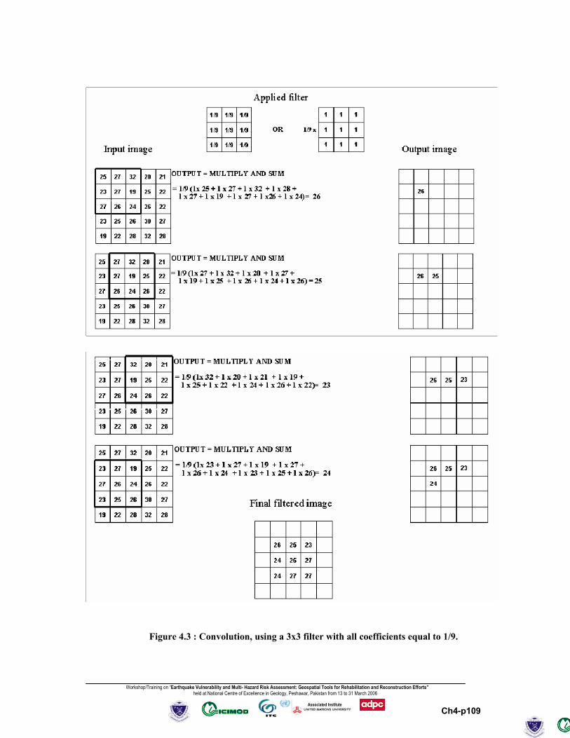
value replaces the original value of the central pixel. This operation is called convolution. Figure 4.3 illustrates the convolution of an image using a 3x3 kernel. The material used for this exercise consists of a Landsat ETM+ 4 band: etmb4.
Low pass filters
To remove the high frequency components in an image, a standard low pass smoothing filter is used. In this activity a 3x3 average filter is going to be used.
• In the Operation-tree, expand Image Processing and double-click the Filter operation. The Filtering dialog box appears.
• Select Raster Map etmb4, use the Linear Filter Type and the standard low pass filter Avg3x3. Enter etmb4_average as Output Raster Map and click the Show button.
• Display the filtered and the unfiltered image next to each other and make a visual comparison.
Create and apply a user-defined low pass filter
It is also possible to create and apply your own filter. A 3x3 low pass filter of the weighted mean type will be created and applied to the image.
• Open the Create Filter dialog box by selecting New Filter in the Operation-list.
• Enter the name Weightmean for the filter to be created, accept the defaults and click OK. The Filter editor is opened.
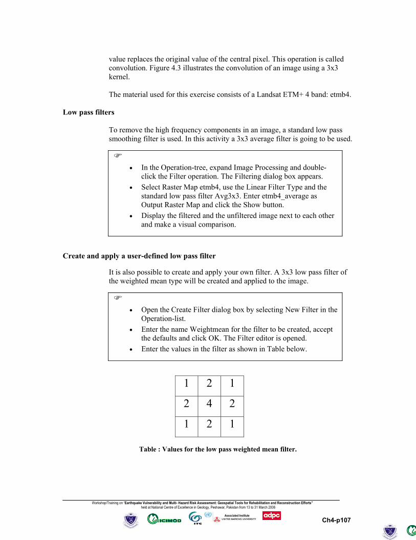
• Enter the values in the filter as shown in Table below.
1 2 1
2 4 2
1 2 1
Table : Values for the low pass weighted mean filter.
Workshop/Training on “Earthquake Vulnerability and Multi- Hazard Risk Assessment: Geospatial Tools for Rehabilitation and Reconstruction Efforts” held at National Centre of Excellence in Geology, Peshawar, Pakistan from 13 to 31 March 2006
Ch4-p108
Associated Institute
• Specify 0.0625 as Gain and close the Filter editor.
What is the function of the gain value?
• Filter the image etmb4 using the smoothing filter just defined.
Select the created filter Weightmean from the Filter Name list box. The Domain for the output map is Image. Type Weightmean as Output Raster Map and click the Show button.
• Compare this filtered image with the image filtered using the standard smoothing filter.
High pass filters
To enhance the high frequency components in an image, a standard high pass filter is used. The applied filter is a 3x3 edge enhancement filter with a central value of 16, eight surrounding values of -1 and a gain of 0.125.
• Open the Filtering dialog box by selecting the Filter operation
in the Operation-list. • Select Raster Map etmb4 and select the Linear filter Edgesenh.
Enter the name Edge for the Output Raster Map. The Domain should be Value (negative values are possible!).
• Accept the default value range and precision and click the Show button. The raster map Edge is calculated and the Display Options - Raster Map dialog box is opened.
• Use a Gray Representation, accept all other defaults and click OK.
• Display the unfiltered and the filtered image next to each other and make a visual comparison.
• Close both map windows afterwards.
Workshop/Training on “Earthquake Vulnerability and Multi- Hazard Risk Assessment: Geospatial Tools for Rehabilitation and Reconstruction Efforts” held at National Centre of Excellence in Geology, Peshawar, Pakistan from 13 to 31 March 2006
Ch4-p109
Associated Institute
Figure 4.3 : Convolution, using a 3x3 filter with all coefficients equal to 1/9.

Workshop/Training on “Earthquake Vulnerability and Multi- Hazard Risk Assessment: Geospatial Tools for Rehabilitation and Reconstruction Efforts” held at National Centre of Excellence in Geology, Peshawar, Pakistan from 13 to 31 March 2006
Ch4-p110
Associated Institute
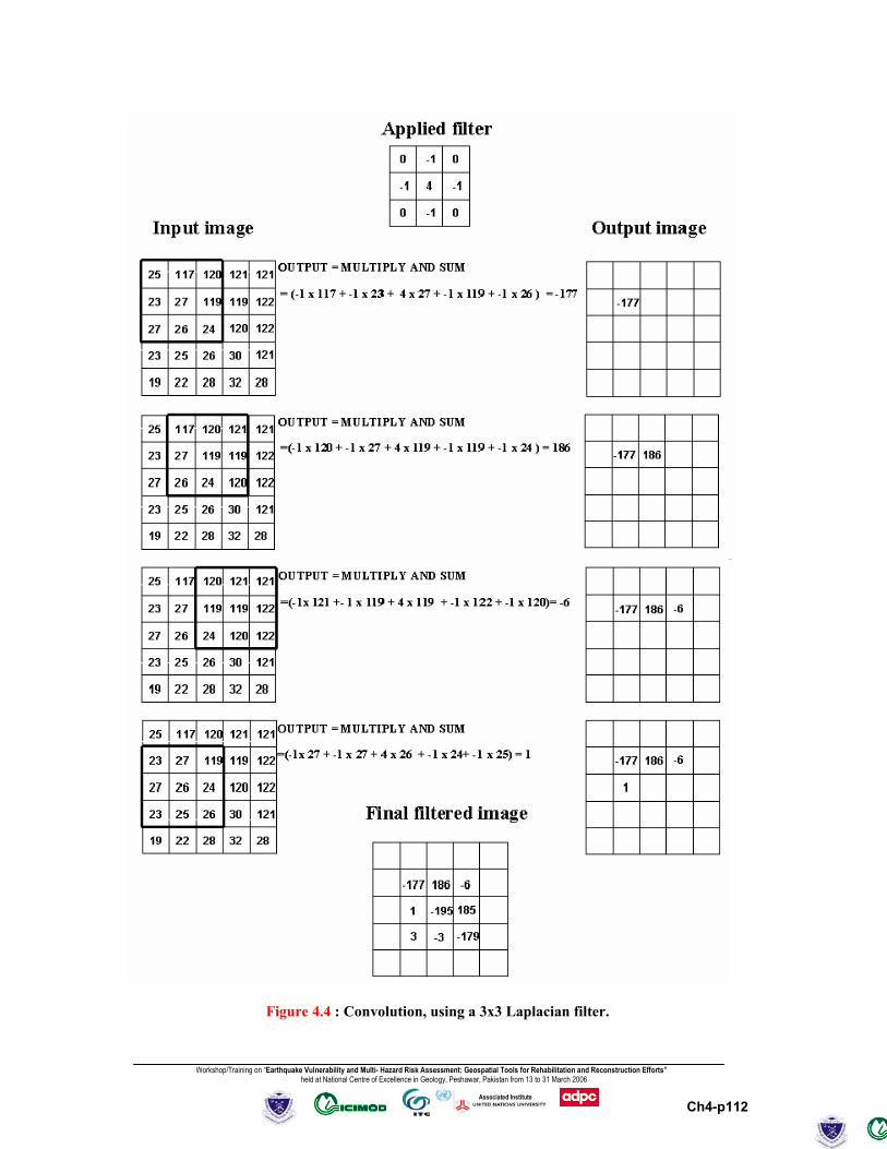
Create and apply a user-defined Laplace filter
Table below gives an example of a 3x3 Laplace filter. The product (sum) of the applied filter is zero. A gain factor to correct the effect of the filter coefficients is therefore not necessary. When these types of filters are applied, the resulting values can be both negative and positive. It is for this reason that ILWIS stores the results of these computations in maps with a value domain. A 3x3 high pass filter of the Laplacian type (the Laplace Plus filter) will be created and applied to the image.
• Open the Create Filter dialog box by selecting New Filter in the
Operation-list. • Enter the Filter Name Laplace_plus accept all other defaults
and Click Show. The Filter editor will be displayed. • In the empty filter enter the values as given in the table below.
Table : Values for the Laplace Plus filter.
0 -1 0
-1 5 -1
0 -1 0
• Accept the default Gain and close the Filter editor.
What is the function of the gain value here?
• Filter image etmb4 using the previously defined Laplace_plus
filter. Use Domain Value and the default value range and step size.
• Filter image etmb4 using a standard Laplace filter. Use the
Workshop/Training on “Earthquake Vulnerability and Multi- Hazard Risk Assessment: Geospatial Tools for Rehabilitation and Reconstruction Efforts” held at National Centre of Excellence in Geology, Peshawar, Pakistan from 13 to 31 March 2006
Ch4-p111
Associated Institute
Domain Value and the default value range and precision. • Compare both filtered images by displaying them in two
different map windows using a Gray Representation. • Close the windows after finishing the exercise.
Directional filters
A directional filter is used to enhance specific linear trends. They are designed in such a way that edges running in a certain direction are enhanced. To enhance lineaments running north-south, an x-gradient filter can be used.
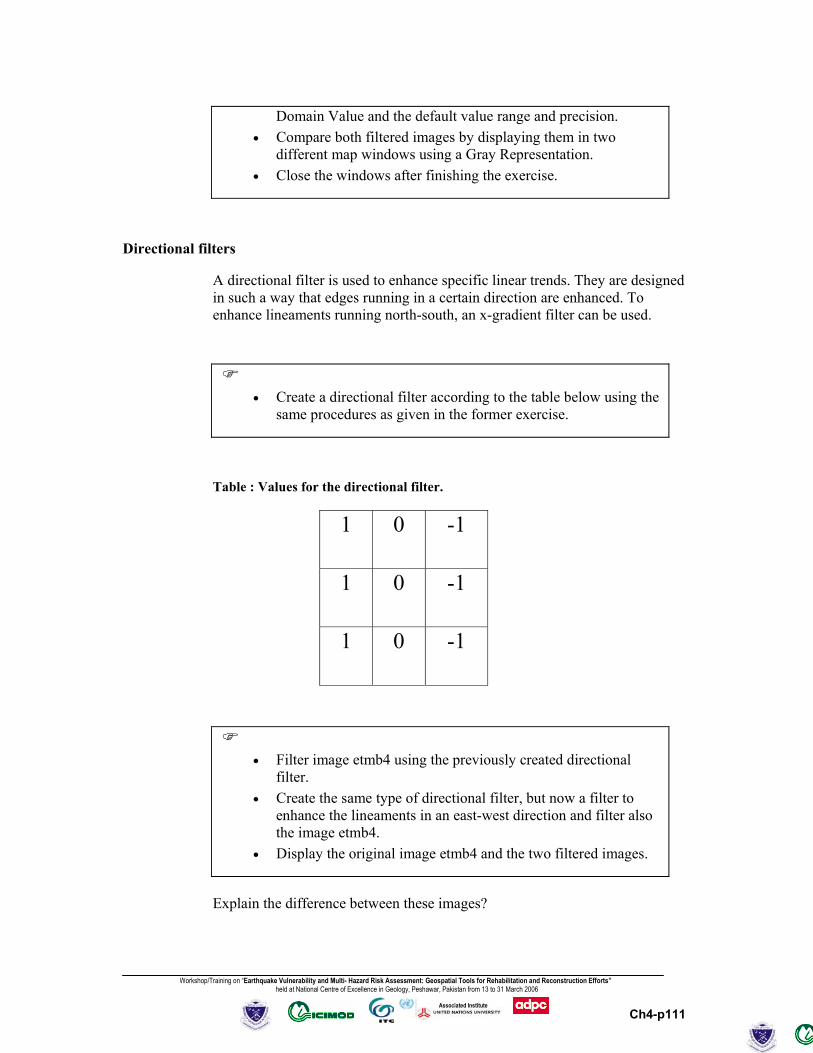
• Create a directional filter according to the table below using the
same procedures as given in the former exercise.
Table : Values for the directional filter.
1 0 -1
1 0 -1
1 0 -1
• Filter image etmb4 using the previously created directional
filter. • Create the same type of directional filter, but now a filter to
enhance the lineaments in an east-west direction and filter also the image etmb4.
• Display the original image etmb4 and the two filtered images.
Explain the difference between these images?
Workshop/Training on “Earthquake Vulnerability and Multi- Hazard Risk Assessment: Geospatial Tools for Rehabilitation and Reconstruction Efforts” held at National Centre of Excellence in Geology, Peshawar, Pakistan from 13 to 31 March 2006
Ch4-p112
Associated Institute
Figure 4.4 : Convolution, using a 3x3 Laplacian filter.
Workshop/Training on “Earthquake Vulnerability and Multi- Hazard Risk Assessment: Geospatial Tools for Rehabilitation and Reconstruction Efforts” held at National Centre of Excellence in Geology, Peshawar, Pakistan from 13 to 31 March 2006
Ch4-p113
Associated Institute
Summary: Image enhancement
- Contrast enhancement, also called global enhancement, transforms the raw data using the statistics computed over the whole data set.
- Techniques used for a contrast enhancement are: the linear stretching technique and histogram equalization. To enhance specific data ranges showing certain land cover types the piece-wise linear contrast stretch can be applied. - The linear stretch is the simplest contrast enhancement. A DN value in the low end of the original histogram is assigned to extreme black, and a value at the high end is assigned to extreme white.
- The histogram equalization technique is a non-linear stretch. In this method, the DN values are redistributed on the basis of their frequency. More different gray tones are assigned to the frequently occurring DN values of the histogram.
- Spatial enhancement procedures result in modification of an image pixel value, based on the pixel values in its immediate vicinity (local enhancement).
- Low pass filters are designed to emphasize low frequency features and to suppress the high frequency component of an image. High pass filters do just the reverse.
- Two classes of high-pass filters can be distinguished: gradient (or directional) filters and Laplacian (or non-directional) filters.
- Gradient filters are directional filters and are used to enhance specific linear trends.
- Laplacian filters are non-directional filters because they enhance linear features having almost any direction in an image.
- A filter usually consists of a 3x3 array (sometimes called kernel) of coefficients or weighting factors.
- Each pixel value is multiplied by the corresponding coefficient in the filter. The 9 values are summed and the resulting value replaces the original value of the central pixel. This operation is called convolution.

Workshop/Training on “Earthquake Vulnerability and Multi- Hazard Risk Assessment: Geospatial Tools for Rehabilitation and Reconstruction Efforts” held at National Centre of Excellence in Geology, Peshawar, Pakistan from 13 to 31 March 2006
Ch4-p114
Associated Institute
3.3 Visualizing multi-band images
In this section, the objective is to understand the concept of color composites and to be able to create different color composites. The spectral information stored in the separate bands can be integrated by combining them into a color composite. Many combinations of bands are possible. The spectral information is combined by displaying each individual band in one of the three primary colors: Red, Green and Blue. A specific combination of bands used to create a color composite image is the so-called False Color Composite (FCC). In a FCC, the red color is assigned to the nearinfrared band, the green color to the red visible band and the blue color to the green visible band. The green vegetation will appear reddish, the water bluish and the (bare) soil in shades of brown and gray. For SPOT multi-spectral imagery, the bands 1, 2 and 3 are displayed respectively in blue, green and red. A combination used very often for TM and ETM+ imagery is the one that displays in red, green and blue the respective bands 4, 3 and 2. Other band combinations are also possible. Some combinations give a color output that resembles natural colors: water is displayed as blue, (bare) soil as red and vegetation as green. Hence this combination leads to a so-called Pseudo Natural Color Composite. Bands of different images (from different imaging systems or different dates), or layers created by band rationing or Principal Component Analysis, can also be combined using the color composite technique. An example could be the multi-temporal combination of vegetation indices for different dates, or the combination of two ETM+ multi-spectral bands with a ETM+ PAN band, (giving in one color image the spectral information of the multispectral bands combined with the higher spatial resolution of the panchromatic band).
3.3.1 Color composites
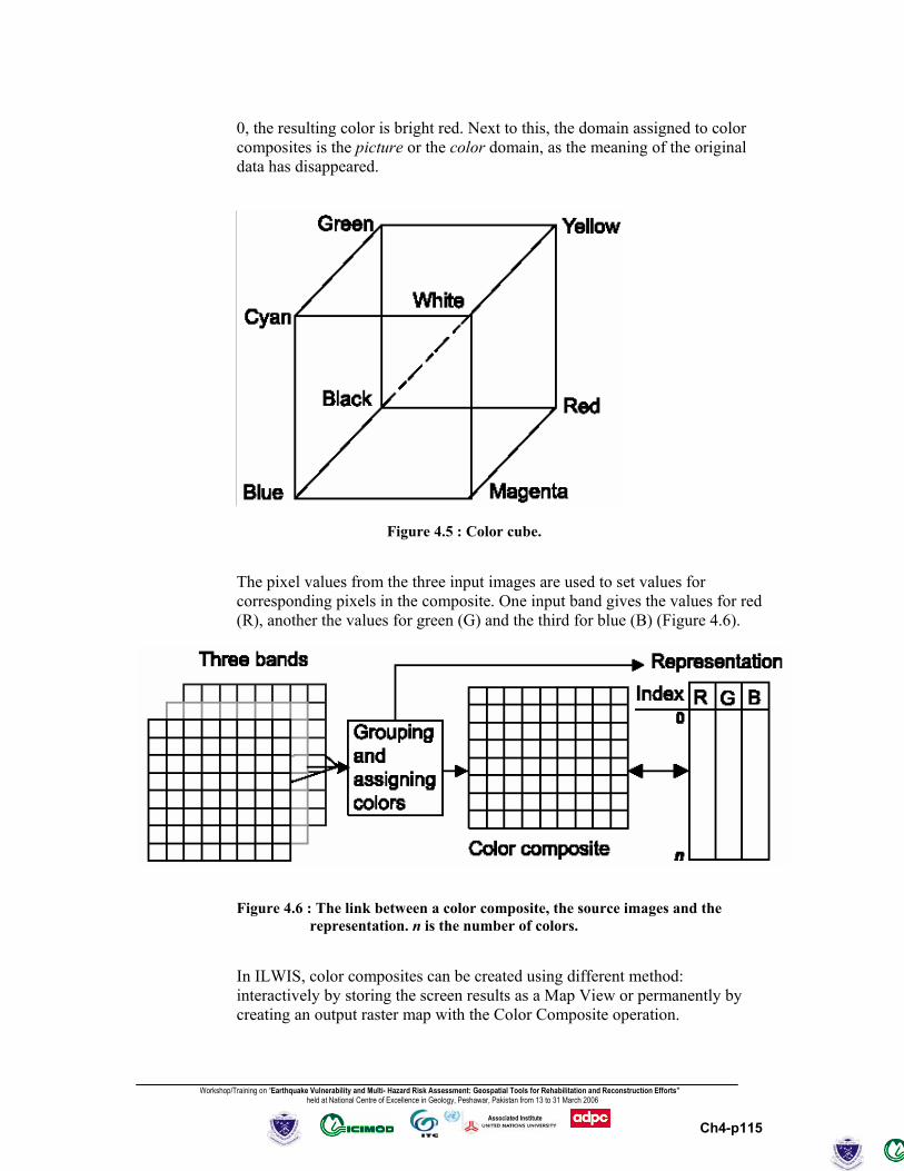
Color composites are created and displayed on the screen, by combining the spectral values of three individual bands. Each band is displayed using one of the primary colors. In Figure 4.5 the color cube is represented and the primary additive (Red, Green and Blue) and subtractive colors (Yellow, Magenta, Cyan) are given. A combination of pixels with high DN values for the individual bands results in a light color. Combining pixels with low DN values produces a dark color. Each point inside the cube produces a different color, depending on the specific contribution of red, green and blue it contains. In ILWIS the relationship between the pixel values of multi-band images and colors, assigned to each pixel, is stored in the representation. A representation stores the values for red, green, and blue. The value for each color represents the relative intensity, ranging from 0 to 255. The three intensities together define the ultimate color, i.e. if the intensity of red = 255, green = 0 and blue =
Workshop/Training on “Earthquake Vulnerability and Multi- Hazard Risk Assessment: Geospatial Tools for Rehabilitation and Reconstruction Efforts” held at National Centre of Excellence in Geology, Peshawar, Pakistan from 13 to 31 March 2006
Ch4-p115
Associated Institute
0, the resulting color is bright red. Next to this, the domain assigned to color composites is the picture or the color domain, as the meaning of the original data has disappeared.
Figure 4.5 : Color cube.
The pixel values from the three input images are used to set values for corresponding pixels in the composite. One input band gives the values for red (R), another the values for green (G) and the third for blue (B) (Figure 4.6).
Figure 4.6 : The link between a color composite, the source images and the representation. n is the number of colors. In ILWIS, color composites can be created using different method: interactively by storing the screen results as a Map View or permanently by creating an output raster map with the Color Composite operation.

Workshop/Training on “Earthquake Vulnerability and Multi- Hazard Risk Assessment: Geospatial Tools for Rehabilitation and Reconstruction Efforts” held at National Centre of Excellence in Geology, Peshawar, Pakistan from 13 to 31 March 2006
Ch4-p116
Associated Institute
Interactive false and pseudo natural color composites
In the exercises below, both an interactive false color composite and an interactive pseudo natural color composite, will be created using Landsat ETM+ bands. For the creation of the false color composite, three ETM+ bands have to be selected. Enter the corresponding ETM+ bands for the spectral ranges indicated in Table below.
. Table below: Spectral ranges for selected ETM+ bands and color assignment
for a false color composite.
Spectral range ETM+ band number To be shown in Near infrared Visible Red Visible Green
Which bands have to be selected, to create an interactive pseudo natural color composite using three ETM+ bands? Write down the color assignment in Table below. Table: Spectral ranges for selected ETM+ bands and color assignment
for a pseudo natural color composite.
Spectral range ETM+ band number To be shown in
Visible Red Visible Green Visible Blue
In this exercise, an interactive color composite is created using ETM+ band 4, 3 and 2. Red is assigned to the near infrared band, green to the red, and blue to the green visible bands. The created color composite image should give a better visual impression of the imaged surface compared to the use of a single band image. Before you can create an interactive color composite you should first create a map list.
• In the Operation-tree expand the Create item and double-click New Map List. The Create Map List dialog box is opened.
• Type etmbands in the text box Map List. In the left-hand list box select the ETM+ images etmb1 to etmb7 and press the > button. The ETM+ images of band 1 through 7 will appear in the list box on the right side. Click OK.
To display the map list as a color composite:
Workshop/Training on “Earthquake Vulnerability and Multi- Hazard Risk Assessment: Geospatial Tools for Rehabilitation and Reconstruction Efforts” held at National Centre of Excellence in Geology, Peshawar, Pakistan from 13 to 31 March 2006
Ch4-p117
Associated Institute
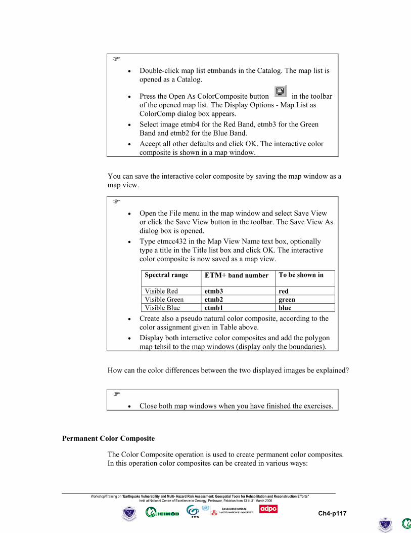
• Double-click map list etmbands in the Catalog. The map list is
opened as a Catalog.
• Press the Open As ColorComposite button in the toolbar of the opened map list. The Display Options - Map List as ColorComp dialog box appears.
• Select image etmb4 for the Red Band, etmb3 for the Green Band and etmb2 for the Blue Band.
• Accept all other defaults and click OK. The interactive color composite is shown in a map window.
You can save the interactive color composite by saving the map window as a map view.
• Open the File menu in the map window and select Save View
or click the Save View button in the toolbar. The Save View As dialog box is opened.
• Type etmcc432 in the Map View Name text box, optionally type a title in the Title list box and click OK. The interactive color composite is now saved as a map view.
Spectral range ETM+ band number To be shown in
Visible Red etmb3 red Visible Green etmb2 green Visible Blue etmb1 blue
• Create also a pseudo natural color composite, according to the color assignment given in Table above.
• Display both interactive color composites and add the polygon map tehsil to the map windows (display only the boundaries).
How can the color differences between the two displayed images be explained?
• Close both map windows when you have finished the exercises.
Permanent Color Composite
The Color Composite operation is used to create permanent color composites. In this operation color composites can be created in various ways:

Workshop/Training on “Earthquake Vulnerability and Multi- Hazard Risk Assessment: Geospatial Tools for Rehabilitation and Reconstruction Efforts” held at National Centre of Excellence in Geology, Peshawar, Pakistan from 13 to 31 March 2006
Ch4-p118
Associated Institute
- Standard Linear Stretching; - Standard Histogram Equalization; - Dynamic; - 24 Bit RGB Linear Stretching; - 24 Bit RGB Histogram Equalization; - 24 Bit HSI.
The different methods of creating a color composite are merely a matter of scaling the input values over the output colors. The exact methods by which this is done are described the ILWIS Help topic: “Color Composite: Algorithm”.
• In the Operation-tree, open the Image Processing item, and
double-click the Color Composite operation. The Color Composite dialog box is opened.
• Select image etmb4 for the Red Band, etmb3 for the Green Band and etmb2 for the Blue Band.
• Type etmccp432 in the Output Raster Map text box, accept all other default and click Show. The permanent color composite is calculated and the Display Options - Raster Map dialog appears.
• Click OK to display the map and close it after you have seen the result.
Summary: Visualizing multi-band images
- The spectral information stored in the separate bands can be integrated by combining them into a color composite. Many combinations of bands are possible. The spectral information is combined by displaying each individual band in one of the three primary colors: red, green and blue.
- In a False Color Composite (FCC), the red color is assigned to the
near-infrared band, the green color to the red visible band and the blue color to the green visible band.
- In a Pseudo Natural Color Composite, the output resembles natural
colors.: water is displayed in blue, (bare) soil as red and vegetation as green.
- In ILWIS, there are two ways in which you can display or create a color
composite: interactive by showing a Map List as Color Composite and permanent by using the Color Composite operation.
Workshop/Training on “Earthquake Vulnerability and Multi- Hazard Risk Assessment: Geospatial Tools for Rehabilitation and Reconstruction Efforts” held at National Centre of Excellence in Geology, Peshawar, Pakistan from 13 to 31 March 2006
Ch4-p119
Associated Institute
3.4 Geometric corrections and image referencing
Remote sensing data is affected by geometric distortions due to sensor geometry, scanner and platform instabilities, earth rotation, earth curvature, etc. Some of these distortions are corrected by the image supplier and others can be corrected referencing the images to existing maps. Remotely sensed images in raw format contain no reference to the location of the data. In order to integrate these data with other data in a GIS, it is necessary to correct and adapt them geometrically, so that they have comparable resolution and projections as the other data sets. The geometry of a satellite image can be ‘distorted’ with respect to a north-south oriented map:
- Heading of the satellite orbit at a given position on Earth (rotation). - Change in resolution of the input image (scaling). - Difference in position of the image and map (shift). - Skew caused by earth rotation (shear).
The different distortions of the image geometry are not realized in certain sequence, but happen all together and, therefore, cannot be corrected stepwise. The correction of ‘all distortions’ at once, is executed by a transformation which combines all the separate corrections. The transformation most frequently used to correct satellite images, is a first order transformation also called affine transformation. This transformation can be given by the following polynomials:
X = a0 + a1rn + a2cn Y = b0 + b1rn + b2cn
Where, rn is the row number, cn is the column number, X and Y are the map coordinates. To define the transformation, it will be necessary to compute the coefficients of the polynomials (e.g. a0, a1, a2, b0, b1 and b2). For the computations, a number of points have to be selected that can be located accurately on the map (X, Y) and which are also identifiable in the image (row, column). The minimum number of points required for the computation of coefficients for an affine transform is three, but in practice you need more. By selecting more points than required, this additional data is used to get the optimal transformation with the smallest overall positional error in the selected points. These errors will appear because of poor positioning of the mouse pointer in an image and by inaccurate measurement of coordinates in a map. The overall accuracy of the transformation is indicated by the average of the errors in the reference points: The so-called Root Mean Square Error (RMSE) or Sigma.
Workshop/Training on “Earthquake Vulnerability and Multi- Hazard Risk Assessment: Geospatial Tools for Rehabilitation and Reconstruction Efforts” held at National Centre of Excellence in Geology, Peshawar, Pakistan from 13 to 31 March 2006
Ch4-p120
Associated Institute
If the accuracy of the transformation is acceptable, then the transformation is linked with the image and a reference can be made for each pixel to the given coordinate system, so the image is geo-referenced. After geo-referencing, the image still has its original geometry and the pixels have their initial position in the image, with respect to row and column indices. In case the image should be combined with data in another coordinate system or georeference, then a transformation has to be applied. This results in a ‘new’ image where the pixels are stored in a new row/column geometry, which is related to the other georeference (containing information on the coordinates and pixel size). This new image is created by applying an interpolation method called resampling. The interpolation method is used to compute the radiometric values of the pixels, in the new image based on the DN values in the original image. After this action, the new image is called geo-coded and it can be overlaid with data having the same coordinate system. ____________________________________________________________ ! In case of satellite imagery from optical systems, it is advised to use a linear transformation. Higher order transformations need much more computation time and in many cases they will enlarge errors. The reference points should be well distributed over the image to minimize the overall error. A good choice is a pattern where the points are along the borders of the image and a few in the center. ____________________________________________________________
3.4.1 GEOREFERENCE
To add coordinates to a satellite image, to a scanned map, or to a scanned photograph when you do not have a Digital Terrain Model (DTM), create a georeference tiepoints. A georeference stores the relation between locations in the image (row, column) and real world coordinates (X, Y). These locations are called tiepoints or ground control points. A georeference uses a coordinate system.
By creating and adding tiepoints to a color composite, one band of a satellite image, a scanned map or a scanned photograph, the tiepoint coordinates are added to the image, photo or map which was specified as background map.
When you were successful in creating a georef tiepoints for a color composite, a band of a satellite image, a scanned map or a scanned photograph, you can:
• see the coordinates according to the created georeference tiepoints on the status bar of the map window;
• display any type of vector data on top of the map;
Workshop/Training on “Earthquake Vulnerability and Multi- Hazard Risk Assessment: Geospatial Tools for Rehabilitation and Reconstruction Efforts” held at National Centre of Excellence in Geology, Peshawar, Pakistan from 13 to 31 March 2006
Ch4-p121
Associated Institute
• create new vector data using the georeferenced image as background; • update vector data using the georeferenced image as background; • use the map in pixel info; • rasterize any vector data on this georeference (for map calculations); • you can also resample the image which has a georeference tiepoints to a
georeference corners, or vice versa, in order to perform raster operations in which raster maps with different georeferences need to be combined;
• screen digitize on satellite images or on scanned photographs or scanned photographs which have a georef tiepoints.
Geo-referencing using corner coordinates
When an image (raster map) is created, either by a satellite, airborne scanner or by an office scanner, the image is stored in row and column geometry in raster format. There is no relationship between the rows/columns and real world coordinates (UTM, geographic coordinates, or any other reference map projection). In a process called geo-referencing the relation between row and column numbers and real world coordinates are established. In general, five approaches can be followed:
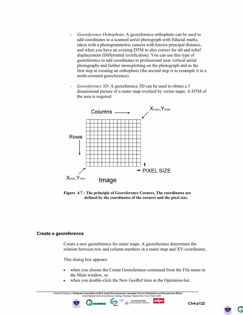
- Georeference Corners: Specifying the coordinates of the lower left (as xmin, ymin) and upper right corner (as xmax, ymax) of the raster image and the actual pixel size (see Figure 4.7, 4.8). A georeference corners is always north-oriented and should be used when rasterizing point, segment, or polygon maps and usually also as the output georeference during resampling.
- Georeference Tiepoints: Specifying reference points in an image so that
specific row/column numbers obtain a correct X, Y coordinate. All other rows and columns then obtain an X, Y coordinate by an affine, second order or projective transformation as specified by the georeference tiepoints. A georeference tiepoints can be used to add coordinates to a satellite image or to a scanned photograph and when you do not have a DTM. This type of georeference can be used to resample (satellite) images to another georeference (e.g. to a georeference corners) or for screen digitizing.
- Georeference Direct Linear: A georeference direct linear can be used to
add coordinates to a scanned photograph which was taken with a normal camera, and when you have an existing DTM to also correct for tilt and relief displacement (Direct Linear Transformation). With this type of georeference you can for instance add coordinates to small format aerial photographs without fiducial marks and for subsequent screen digitizing or to resample the photograph to another georeference (e.g. to a georeference corners).
Workshop/Training on “Earthquake Vulnerability and Multi- Hazard Risk Assessment: Geospatial Tools for Rehabilitation and Reconstruction Efforts” held at National Centre of Excellence in Geology, Peshawar, Pakistan from 13 to 31 March 2006
Ch4-p122
Associated Institute
- Georeference Orthophoto: A georeference orthophoto can be used to add coordinates to a scanned aerial photograph with fiducial marks, taken with a photogrammetric camera with known principal distance, and when you have an existing DTM to also correct for tilt and relief displacement (Differential rectification). You can use this type of georeference to add coordinates to professional near vertical aerial photographs and further monoplotting on the photograph and as the first step in creating an orthophoto (the second step is to resample it to a north-oriented georeference).
- Georeference 3D: A georeference 3D can be used to obtain a 3
dimensional picture of a raster map overlaid by vector maps. A DTM of the area is required.
Figure 4.7 : The principle of Georeference Corners. The coordinates are defined by the coordinates of the corners and the pixel size.
Create a georeference
Create a new georeference for raster maps. A georeference determines the relation between row and column numbers in a raster map and XY-coordinates.
This dialog box appears:
• when you choose the Create Georeference command from the File menu in the Main window, or
• when you double-click the New GeoRef item in the Operation-list.
Workshop/Training on “Earthquake Vulnerability and Multi- Hazard Risk Assessment: Geospatial Tools for Rehabilitation and Reconstruction Efforts” held at National Centre of Excellence in Geology, Peshawar, Pakistan from 13 to 31 March 2006
Ch4-p123
Associated Institute
This dialog box can be used to create:
• a georeference corners: to be used during rasterize operations, or as a North-oriented georeference to which you want to resample raster maps, or
• a georeference tiepoints: to add coordinates to a satellite image or a scanned photograph without using a DTM, or
• a georeference direct linear: to add coordinates to a scanned photograph while using a DTM, or
• a georeference orthophoto: to add coordinates to a scanned aerial photograph while using a DTM and camera parameters, or
• a georeference 3D: to obtain a three-dimensional view of your study area.
Dialog box options:
Georeference name: Type a new name for the georeference. In case of a georeference, which will be used for multiple raster maps of the same size and of the same area, it is advised to enter a georeference name that applies to all maps (e.g. the name of the study area).
Description: Type a description for the georeference. The description is visible on the status bar of the Main window when moving the mouse pointer over the georeference in the Catalog.
Georef Corners: Select Georef Corners to create a North-oriented georeference, for example when rasterizing point, segment or polygon maps, or for the output of a Resampling operation.
Georef Tiepoints: Select Georef Tiepoints when you want to add coordinates to a satellite image or to a scanned photograph and when you do not have a DTM. This type of georeference can be used to add coordinates to satellite imagery and for subsequent screen digitizing or to resample the image to another georeference (e.g. to a georef corners).
Georef Direct Linear: Select Georef Direct Linear when you want to add coordinates to a scanned photograph which was taken with a normal camera, and when you have an existing DTM to also correct for tilt and relief displacement (Direct Linear Transformation). This type of georeference can for instance be used to add coordinates to small format aerial photographs and for subsequent screen digitizing or to resample the photograph to another georeference (e.g. to a georef corners).
Georef OrthoPhoto: Select Georef Orthophoto when you want to add coordinates to a scanned aerial photograph with fiducial marks, taken with a photogrammetric camera with known principal distance, and when you have an existing DTM to also correct for tilt and relief displacement (Differential rectification). This type of georeference can be used to add coordinates to professional near vertical aerial photographs and further monoplotting on the photograph or for

Workshop/Training on “Earthquake Vulnerability and Multi- Hazard Risk Assessment: Geospatial Tools for Rehabilitation and Reconstruction Efforts” held at National Centre of Excellence in Geology, Peshawar, Pakistan from 13 to 31 March 2006
Ch4-p124
Associated Institute
creating an orthophoto (resampling). Georef 3D display: Select Georef 3D when you want to make a three-dimensional
picture of your study area using a Digital Elevation Model.
For Georef Corners:
Coordinate system: Select a coordinate system in which this georeference fits. If you do not have a coordinate system yet, it is advised to create one first. To create a coordinate system, click the create button next to this list box or select the Create Coordinate System command from the File menu in the Main window: the Create Coordinate System dialog box will appear.
Pixel size: Type a pixel size for the new raster map. When you specify for instance 20, the size of each pixel in the raster map will be 20 x 20 m.
Map boundaries: When an existing coordinate system is selected, the boundary Xmin, Ymin, Xmax and Ymax values of the map are already filled out as defaults. Or type the minimum and maximum X and Y values yourself.
Centers: Select this check box if the four boundary values (Xmin, Ymin, Xmax, Ymax) of this map should refer to the centers of the four corner pixels of the map. Clear this check box if the four boundary values should refer to the outer corners of the four corner pixels of this map.
• Open the File menu in the Main window and select Create,
GeoReference. The Create GeoReference dialog box is opened. • Enter etmpan15m for the GeoReference Name. Note that the
option GeoRef Corners is selected. • Type: GeoReference Corners for the Pakistan Landsat7 path150
row036 ETM+PAN area of 2001 October 07 with 15m pixel size in the text box Description.
• Select GeoRefCorners. • Select Coordinate System utm43wgs84 • Enter 15 in the text box Pixel size • Select Center of Corner pixels
A georeference is linked to a coordinate system; the coordinate system contains the minimum and maximum coordinates of the study area, and

Workshop/Training on “Earthquake Vulnerability and Multi- Hazard Risk Assessment: Geospatial Tools for Rehabilitation and Reconstruction Efforts” held at National Centre of Excellence in Geology, Peshawar, Pakistan from 13 to 31 March 2006
Ch4-p125
Associated Institute
optional projection parameters. It is always advised to create a coordinate system of type Projection for the study area in which you are working, even if you do not have projection information, instead of using the coordinate system Unknown. This is important if you want to transform later on other data that have different coordinate systems and/or projections. If you do not have coordinate systems for northern Pakistan covering Landsat7 path150 row 036 ETM+PAN area you can create the coordinate system utm43wgs84 using UTM Zone 43 and WGS84 Datum and Ellipsoid.
Workshop/Training on “Earthquake Vulnerability and Multi- Hazard Risk Assessment: Geospatial Tools for Rehabilitation and Reconstruction Efforts” held at National Centre of Excellence in Geology, Peshawar, Pakistan from 13 to 31 March 2006
Ch4-p126
Associated Institute
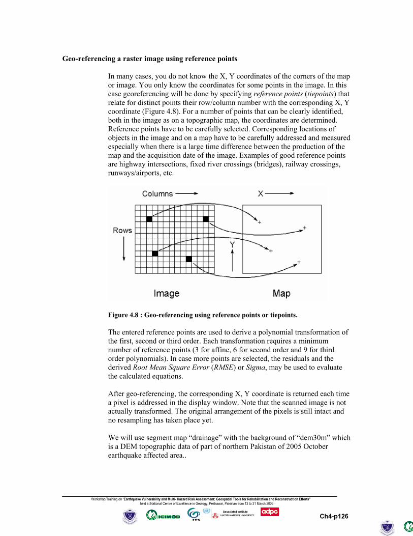
Geo-referencing a raster image using reference points
In many cases, you do not know the X, Y coordinates of the corners of the map or image. You only know the coordinates for some points in the image. In this case georeferencing will be done by specifying reference points (tiepoints) that relate for distinct points their row/column number with the corresponding X, Y coordinate (Figure 4.8). For a number of points that can be clearly identified, both in the image as on a topographic map, the coordinates are determined. Reference points have to be carefully selected. Corresponding locations of objects in the image and on a map have to be carefully addressed and measured especially when there is a large time difference between the production of the map and the acquisition date of the image. Examples of good reference points are highway intersections, fixed river crossings (bridges), railway crossings, runways/airports, etc.
Figure 4.8 : Geo-referencing using reference points or tiepoints.
The entered reference points are used to derive a polynomial transformation of the first, second or third order. Each transformation requires a minimum number of reference points (3 for affine, 6 for second order and 9 for third order polynomials). In case more points are selected, the residuals and the derived Root Mean Square Error (RMSE) or Sigma, may be used to evaluate the calculated equations. After geo-referencing, the corresponding X, Y coordinate is returned each time a pixel is addressed in the display window. Note that the scanned image is not actually transformed. The original arrangement of the pixels is still intact and no resampling has taken place yet. We will use segment map “drainage” with the background of “dem30m” which is a DEM topographic data of part of northern Pakistan of 2005 October earthquake affected area..
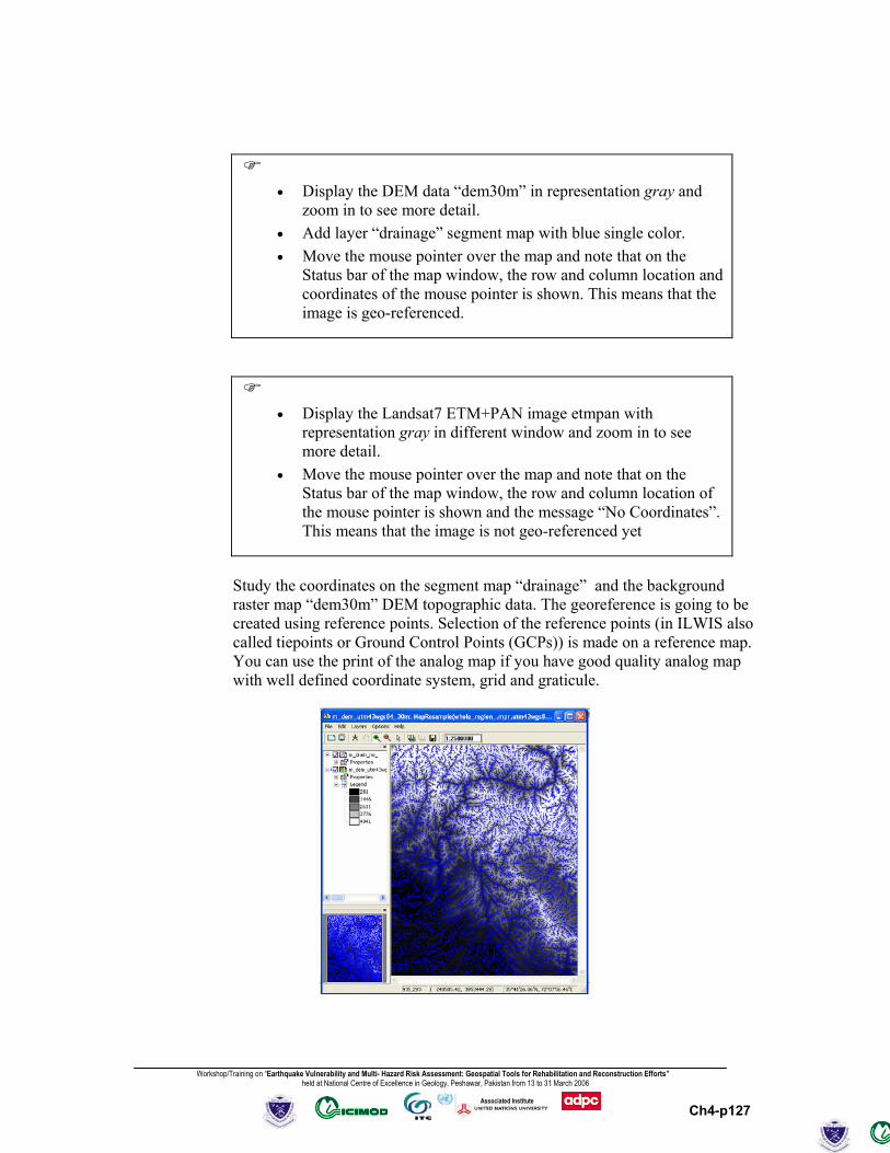
Workshop/Training on “Earthquake Vulnerability and Multi- Hazard Risk Assessment: Geospatial Tools for Rehabilitation and Reconstruction Efforts” held at National Centre of Excellence in Geology, Peshawar, Pakistan from 13 to 31 March 2006
Ch4-p127
Associated Institute
• Display the DEM data “dem30m” in representation gray and
zoom in to see more detail. • Add layer “drainage” segment map with blue single color. • Move the mouse pointer over the map and note that on the
Status bar of the map window, the row and column location and coordinates of the mouse pointer is shown. This means that the image is geo-referenced.
• Display the Landsat7 ETM+PAN image etmpan with
representation gray in different window and zoom in to see more detail.
• Move the mouse pointer over the map and note that on the Status bar of the map window, the row and column location of the mouse pointer is shown and the message “No Coordinates”. This means that the image is not geo-referenced yet
Study the coordinates on the segment map “drainage” and the background raster map “dem30m” DEM topographic data. The georeference is going to be created using reference points. Selection of the reference points (in ILWIS also called tiepoints or Ground Control Points (GCPs)) is made on a reference map. You can use the print of the analog map if you have good quality analog map with well defined coordinate system, grid and graticule.

Workshop/Training on “Earthquake Vulnerability and Multi- Hazard Risk Assessment: Geospatial Tools for Rehabilitation and Reconstruction Efforts” held at National Centre of Excellence in Geology, Peshawar, Pakistan from 13 to 31 March 2006
Ch4-p128
Associated Institute
Georef Tiepoints
This type of georeference can be used to add coordinates to general raster maps (satellite imagery and scanned map). Add a tiepoint, also called ground control point, a tiepoint establishes the relation between a Row Column number in a map and its real world XY- or XYZ-coordinate.
Dialog box:
Row Col: The Row and Column numbers of the position that you clicked in the background image are shown.
X Y: To obtain the XY-coordinate for this tiepoint, either:
• read the XY-coordinate of this position from a paper map (analog map), and type these in the X Y boxes, or
• click at the same position in a map window which already has correct defined coordinates (master/slave) and the X Y boxes are automatically filled out, or
• digitize the same position on a map stuck on the digitizer and the X Y boxes are automatically filled out.
When you already have a (mathematically) sufficient number of tiepoints, and you add a new tiepoint, the dialog box comes up with a suggestion for the XY-coordinates for this point. The suggested XY-coordinate gives an indication of the quality of your existing tiepoints. You should never accept this suggestion but always look up the correct XY-coordinate from a paper map, a master, etc.
Z: When adding a tiepoint to a georef direct linear or a georef orthophoto, select this check box when you want to fill out a Z (height) value for the inserted tiepoint; as a default, the Z-value found in the DTM is given.
Clear this check box when you want to use the height value found in the DTM.
When you click OK, the tiepoint will be added to the tiepoint table.
! Tips:
• To make a tiepoint inactive for this georeference: in column Active, set the value on False by typing an F.
• To check the quality of a georeference tiepoints, you can add a segment map with digitized features on top of the raster map when adding tiepoints. Then, add tiepoints, redraw the map window once in a while and see when the segments fit well enough on your background image.
• To add a created georeference tiepoints to other bands of a satellite image, open the properties of the other bands: in the Properties dialog box, click the Edit Properties button, then select the newly created georeference tiepoints.
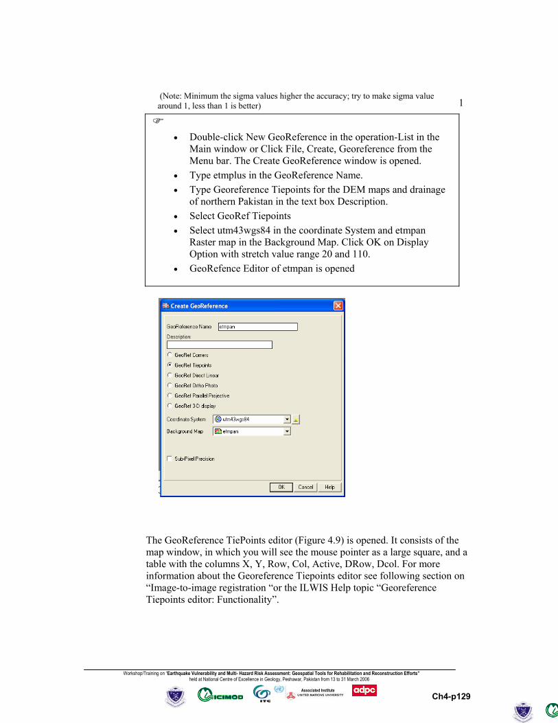
Workshop/Training on “Earthquake Vulnerability and Multi- Hazard Risk Assessment: Geospatial Tools for Rehabilitation and Reconstruction Efforts” held at National Centre of Excellence in Geology, Peshawar, Pakistan from 13 to 31 March 2006
Ch4-p129
Associated Institute
1
• Double-click New GeoReference in the operation-List in the
Main window or Click File, Create, Georeference from the Menu bar. The Create GeoReference window is opened.
• Type etmplus in the GeoReference Name. • Type Georeference Tiepoints for the DEM maps and drainage
of northern Pakistan in the text box Description. • Select GeoRef Tiepoints • Select utm43wgs84 in the coordinate System and etmpan
Raster map in the Background Map. Click OK on Display Option with stretch value range 20 and 110.
• GeoRefence Editor of etmpan is opened
The GeoReference TiePoints editor (Figure 4.9) is opened. It consists of the map window, in which you will see the mouse pointer as a large square, and a table with the columns X, Y, Row, Col, Active, DRow, Dcol. For more information about the Georeference Tiepoints editor see following section on “Image-to-image registration “or the ILWIS Help topic “Georeference Tiepoints editor: Functionality”.
(Note: Minimum the sigma values higher the accuracy; try to make sigma value around 1, less than 1 is better)
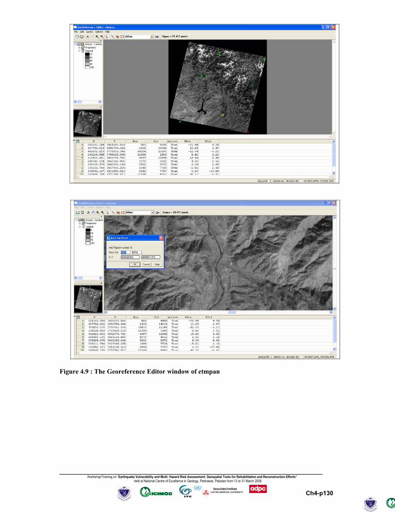
Workshop/Training on “Earthquake Vulnerability and Multi- Hazard Risk Assessment: Geospatial Tools for Rehabilitation and Reconstruction Efforts” held at National Centre of Excellence in Geology, Peshawar, Pakistan from 13 to 31 March 2006
Ch4-p130
Associated Institute
Figure 4.9 : The Georeference Editor window of etmpan
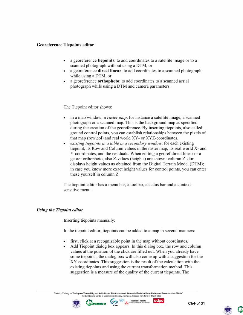
Workshop/Training on “Earthquake Vulnerability and Multi- Hazard Risk Assessment: Geospatial Tools for Rehabilitation and Reconstruction Efforts” held at National Centre of Excellence in Geology, Peshawar, Pakistan from 13 to 31 March 2006
Ch4-p131
Associated Institute
Georeference Tiepoints editor
• a georeference tiepoints: to add coordinates to a satellite image or to a scanned photograph without using a DTM, or
• a georeference direct linear: to add coordinates to a scanned photograph while using a DTM, or
• a georeference orthophoto: to add coordinates to a scanned aerial photograph while using a DTM and camera parameters.
The Tiepoint editor shows:
• in a map window: a raster map, for instance a satellite image, a scanned photograph or a scanned map. This is the background map as specified during the creation of the georeference. By inserting tiepoints, also called ground control points, you can establish relationships between the pixels of that map (row,col) and real world XY- or XYZ-coordinates.
• existing tiepoints in a table in a secondary window: for each existing tiepoint, its Row and Column values in the raster map, its real world X- and Y-coordinates, and the residuals. When editing a georef direct linear or a georef orthophoto, also Z-values (heights) are shown: column Z_dtm displays height values as obtained from the Digital Terrain Model (DTM); in case you know more exact height values for control points, you can enter these yourself in column Z.
The tiepoint editor has a menu bar, a toolbar, a status bar and a context-sensitive menu.
Using the Tiepoint editor
Inserting tiepoints manually:
In the tiepoint editor, tiepoints can be added to a map in several manners:
• first, click at a recognizable point in the map without coordinates, • Add Tiepoint dialog box appears. In this dialog box, the row and column
values at the position of the click are filled out. When you already have some tiepoints, the dialog box will also come up with a suggestion for the XY-coordinates. This suggestion is the result of the calculation with the existing tiepoints and using the current transformation method. This suggestion is a measure of the quality of the current tiepoints. The

Workshop/Training on “Earthquake Vulnerability and Multi- Hazard Risk Assessment: Geospatial Tools for Rehabilitation and Reconstruction Efforts” held at National Centre of Excellence in Geology, Peshawar, Pakistan from 13 to 31 March 2006
Ch4-p132
Associated Institute
suggestion is merely a suggestion, it is advised to enter your own XY-coordinates to prevent false accuracy.
Then:
• click at the same position in a map which already has correct XY-coordinates and which is displayed in another map window (Master/Slave), or
• digitize the same point in an analog paper map on a digitizer, or • read the correct XY-coordinates for this point from a table or an analog
paper map, and type these XY-coordinates in the dialog box.
When editing a georef direct linear or a georef orthophoto, you can optionally specify a Z-value for the inserted tiepoint; otherwise the height value as found in the DTM is used.
The inserted tiepoint appears in the map window and in the tiepoint table.
For a more detailed description on inserting tiepoints (for instance Master/Slave or using a digitizer, etc.), refer to How to use the Georeference Tiepoints editor.
Inserting tiepoints from file:
When you already have tiepoints (X-coordinates, Y-coordinates, row numbers, column numbers) in a file, it is advised to paste these tiepoints into the tiepoint table of a georeference tiepoints.
For a more detailed description, refer to How to paste coordinates into a georeference tiepoints.
(De) selecting tiepoints:
Column Active in the tiepoint table indicates whether or not a tiepoint is used in the transformation. Include tiepoints by the putting True in column Active; exclude tiepoints by putting False in column Active. You can type T or F in column Active or use the space bar to switch between these.
Changing colors and symbol size of tiepoints and/or fiducial marks:
To change the colors or symbol size of tiepoints or to change the colors of fiducial marks, choose Customize from the Edit menu.

Workshop/Training on “Earthquake Vulnerability and Multi- Hazard Risk Assessment: Geospatial Tools for Rehabilitation and Reconstruction Efforts” held at National Centre of Excellence in Geology, Peshawar, Pakistan from 13 to 31 March 2006
Ch4-p133
Associated Institute
Deleting tiepoints:
To delete a tiepoint, choose Delete Tiepoint from the Edit menu, or click the Delete Tiepoint button in the toolbar. Furthermore, after selecting a tiepoint in the tiepoint table, you can press Del on the keyboard, or use the right mouse button and select Delete from the context-sensitive menu.
Georef Tiepoints: transformation method:
When editing a georef tiepoints, one of the following transformation methods can be selected: conformal, affine, second order bilinear, full second order, third order and projective.
• For satellite images an affine transformation will usually do; • For a scanned photograph (without DTM), a projective transformation is
recommended.
Tiepoint requirements:
• Mathematical minimum number of tiepoints required: o Georef tiepoints: conformal 2; affine 3; second order 4; full second
order 6; third order 10; projective 4. o Georef direct linear: 6 o Georef orthophoto: 3
• You should always insert more tiepoints than is mathematically required. • Tiepoints should be well spread over the map (XY-direction). • For a georef direct linear, the tiepoints should also be well spread in Z-
direction and they should not be coplanar, i.e. in Z-direction, the tiepoints should not be on a (tilted) plane. For more information, see ILWIS objects: georeference Direct Linear.
Inspecting DRow, DCol and Sigma:
Columns DRow and DCol show the difference between calculated Row and Col values and actual Row and Col values in pixels. Very good control points have DRow and DCol values less than 2. Sigma is calculated from these values and the degrees of freedom, and gives a measure for the overall accountability or credibility of the active tiepoints.
! Tips:

Workshop/Training on “Earthquake Vulnerability and Multi- Hazard Risk Assessment: Geospatial Tools for Rehabilitation and Reconstruction Efforts” held at National Centre of Excellence in Geology, Peshawar, Pakistan from 13 to 31 March 2006
Ch4-p134
Associated Institute
1. When you have already a vector map of the area of the image, it can be handy to display this vector map on top of the image while working with the tiepoint editor. When you now
add tiepoints to the image and press the Redraw button , you can judge the quality of the tiepoints.
2. For a georef tiepoints which should be used by all bands of a satellite image: after you have finished adding tiepoints to a background map in the Tiepoint editor, you have to add the created georef tiepoints to all bands of the image. This can be done by opening the Properties sheets of the bands and select the correct georef tiepoints.
3. When finished creating a georeference for an image or a photograph, you can directly create a segment map (choose File, Create in the map window) and start screen digitizing on the image or photo which now uses the created georef tiepoints, georef direct linear or georef orthophoto. When you created a georef orthophoto, the screen digitizing is called monoplotting.
4. When finished editing a georef tiepoints, a georef direct linear or a georef orthophoto, detailed information on transformation or orientation results can be viewed in the Properties dialog box of the georeference: click the Additional Info button.
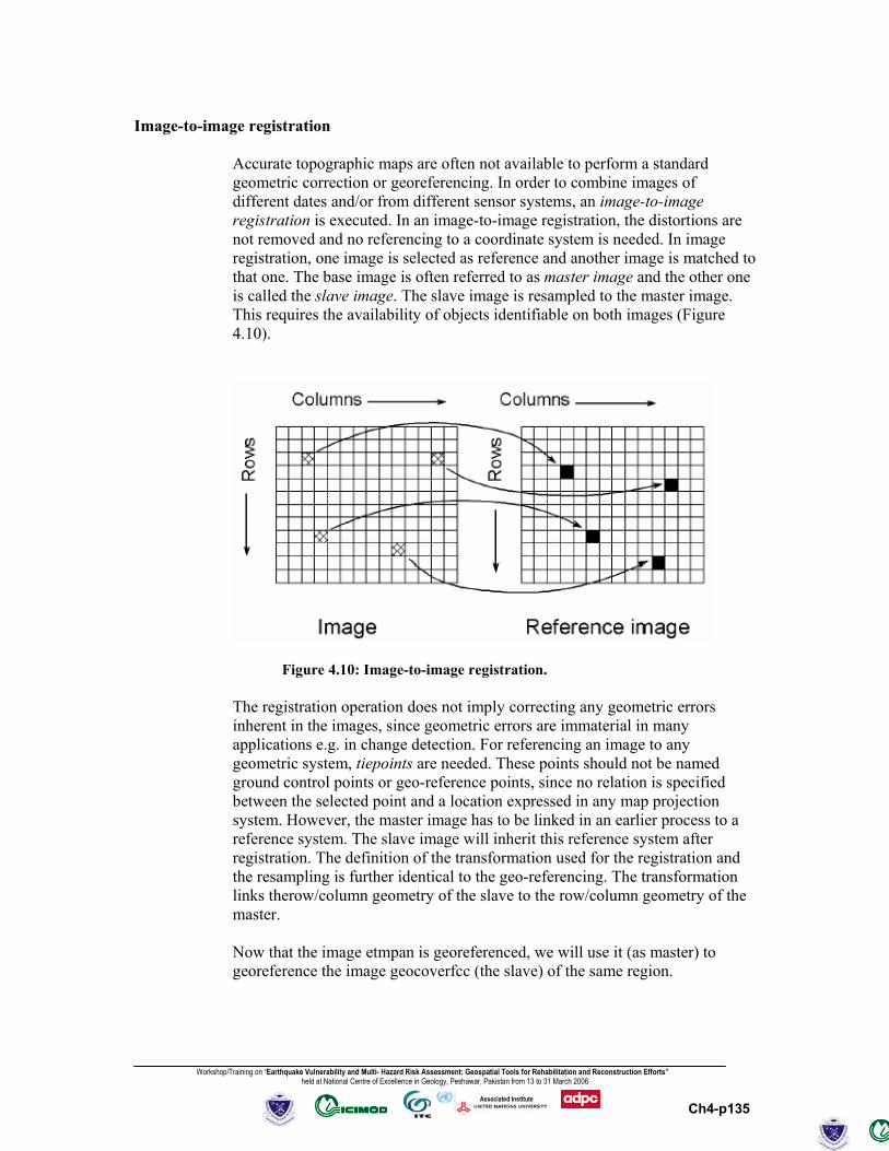
Workshop/Training on “Earthquake Vulnerability and Multi- Hazard Risk Assessment: Geospatial Tools for Rehabilitation and Reconstruction Efforts” held at National Centre of Excellence in Geology, Peshawar, Pakistan from 13 to 31 March 2006
Ch4-p135
Associated Institute
Image-to-image registration
Accurate topographic maps are often not available to perform a standard geometric correction or georeferencing. In order to combine images of different dates and/or from different sensor systems, an image-to-image registration is executed. In an image-to-image registration, the distortions are not removed and no referencing to a coordinate system is needed. In image registration, one image is selected as reference and another image is matched to that one. The base image is often referred to as master image and the other one is called the slave image. The slave image is resampled to the master image. This requires the availability of objects identifiable on both images (Figure 4.10).
Figure 4.10: Image-to-image registration. The registration operation does not imply correcting any geometric errors inherent in the images, since geometric errors are immaterial in many applications e.g. in change detection. For referencing an image to any geometric system, tiepoints are needed. These points should not be named ground control points or geo-reference points, since no relation is specified between the selected point and a location expressed in any map projection system. However, the master image has to be linked in an earlier process to a reference system. The slave image will inherit this reference system after registration. The definition of the transformation used for the registration and the resampling is further identical to the geo-referencing. The transformation links therow/column geometry of the slave to the row/column geometry of the master. Now that the image etmpan is georeferenced, we will use it (as master) to georeference the image geocoverfcc (the slave) of the same region.
Workshop/Training on “Earthquake Vulnerability and Multi- Hazard Risk Assessment: Geospatial Tools for Rehabilitation and Reconstruction Efforts” held at National Centre of Excellence in Geology, Peshawar, Pakistan from 13 to 31 March 2006
Ch4-p136
Associated Institute
• Open satellite image geocoverfcc. • In the map window, open the File menu and select Create,
GeoReference. The Create GeoReference dialog box is opened. • Enter geocoverfcc for the GeoReference Name. • Type: GeoReference for the northern Pakistan area geocoverfcc
image in the text box Description. • Select the option GeoRef Tiepoints. • Select the Coordinate System utm43wgs84 and click OK. The
Georeference Tiepoints editor is appears. • Position the window geocoverfcc and etmpan next to each other
so that you can see both clearly.
At this point you can start entering the reference points (tiepoints) by clicking pixels in the slave (to obtain Row/Column numbers) and then clicking at the same position in the master (to obtain X,Y coordinates). The following procedures can be used to enter tiepoints in the Georeference Tiepoints editor: - Firstly, click with the mouse pointer at a recognizable point in the
background image without coordinates (the slave). The Add Tie Point dialog box appears. In this dialog box, the row and column values at the position of the click are shown. When already sufficient tiepoints are selected, the dialog box will come up with a suggestion for the XY coordinates (which should never be accepted without reflection).
Then:
- Click at the same position in a image of the same area which is already georeferenced (the master) and which is displayed in another map window (in this case the image etmpan), or;
- Digitize the same point in an analog paper map or image which is fixed
onto a digitizer, or; - Read the correct XY coordinates for this point from an analog paper
map/image or a table, and type these XY coordinates in the dialog box.
• Choose a location in the slave image geocoverfcc for which you
can find the coordinate pair in the master image etmpan. • Zoom in on the chosen location, and click the reference point in
the slave image as accurately as possible. The Add Tie Point dialog box appears.
• Go to the map window with the master raster map and click the pixel, which corresponds to that position. In the Add Tie Point dialog box, the correct X and Y coordinates are filled out now.
Workshop/Training on “Earthquake Vulnerability and Multi- Hazard Risk Assessment: Geospatial Tools for Rehabilitation and Reconstruction Efforts” held at National Centre of Excellence in Geology, Peshawar, Pakistan from 13 to 31 March 2006
Ch4-p137
Associated Institute
• Click OK to close the Add Tie Point dialog box. • Repeat this procedure for at least 5 other reference points.
When three control points are entered, a Sigma and residuals (DRow and DCol) are calculated. Columns DRow and DCol show the difference between calculated row and column values and actual row and column values in pixels. Very good control points have DRow and DCol values of less than 2 pixels. The Sigma is calculated from the Drow and DCol values and the degrees of freedom, and gives a measure for the overall accountability or credibility of the active tiepoints. The overall sigma value indicates the accuracy of the transformation. Based on the expected geometric distortions in the background image a transformation method can be selected. By default, an Affine transformation is used. You can choose another transformation method in the Transformation dialog box (Edit menu, or context-sensitive menu) as well as in the drop-down list box in the toolbar of the GeoReference Tiepoints editor. ! For satellite images an affine transformation will usually do. For a scanned photograph (without DTM), a projective transformation is recommended. A tiepoint can be selected or excluded from the transformation computation by putting True or False respectively in the column Active. By excluding tiepoints, you can for instance evaluate the performance of the transformation; assuming that the excluded tiepoints are correctly chosen. Furthermore, in the Georeference Tiepoints editor, good tiepoints are shown in green, medium good tiepoints are shown in yellow, ‘bad’ tiepoints are shown in red, and passive tiepoints are shown in blue. You can set these colors in the Customize Georeference Tiepoints editor dialog box. A tiepoint is considered well positioned if: √(DRow2+DCol2)<=(1.2*Sigma) A tiepoint is considered to have a medium error if: √(1.2*Sigma)<√(DRow2+DCol2)<=(2*Sigma) A tiepoint is considered to have a large error if: √(DRow2+DCol2)>(2*Sigma) A tiepoint can be deleted by clicking its record number and by selecting Edit, Delete Tiepoint, or by pressing <Delete> on the keyboard. If confirmed, the tiepoint will be deleted.
Workshop/Training on “Earthquake Vulnerability and Multi- Hazard Risk Assessment: Geospatial Tools for Rehabilitation and Reconstruction Efforts” held at National Centre of Excellence in Geology, Peshawar, Pakistan from 13 to 31 March 2006
Ch4-p138
Associated Institute
• Inspect the DRow and DCol values and inspect the Sigma. • Close the GeoReference Tiepoints editor when finished. • You will return to the map window. See that the image
geocoverfcc now has coordinates. Move the mouse pointer around in the image and determine for some easy identifiable pixels the accuracy of the transformation. Use the zoom in option if necessary.
If you are doing the georeference multiband image instead of single band as here geocoverfcc or etmpan the georeference created for the one band of the multibands image can also be used for other bands (such as for SPOT, TM, ETM+ images) since all bands refer to the same area and have the same number of rows and columns.
If you are using SPOT or TM or ETM+ image instead of geocoverfcc as slave image then you can georeference one band say spotb3 and then with reference to that you can georeference other bands.
• In the Catalog click spotb1 with the right mouse button and select Properties. In the Properties of Raster Map “spotb1” sheet, change the GeoReference of the image to etmpan. Close the Properties sheet.
• Do the same for spotb2 and close all windows when all three SPOT bands are georeferenced.
Geo-coding a raster image by resampling
After geo-referencing an image, the image will have coordinates for each pixel, but its geometry is not corrected for geometric distortions and not adapted to a master map or image. To create a distortion free adapted image, the transformation that is defined during geo-referencing (see previous exercise) is executed. This process, geocoding, results in a new image in which the pixels are arranged in the geometry of the master image or map, and the resolution is equal to the resolution of the master image or chosen in case the master is a topographic map. The radiometric values or pixel values of the new image are found by resampling the original image using a chosen interpolation method (Figure 4.11). The value for a pixel in the output image is found at a certain position in the input image. This position is computed using the inverse of the transformation that is defined in the geo-referencing process.
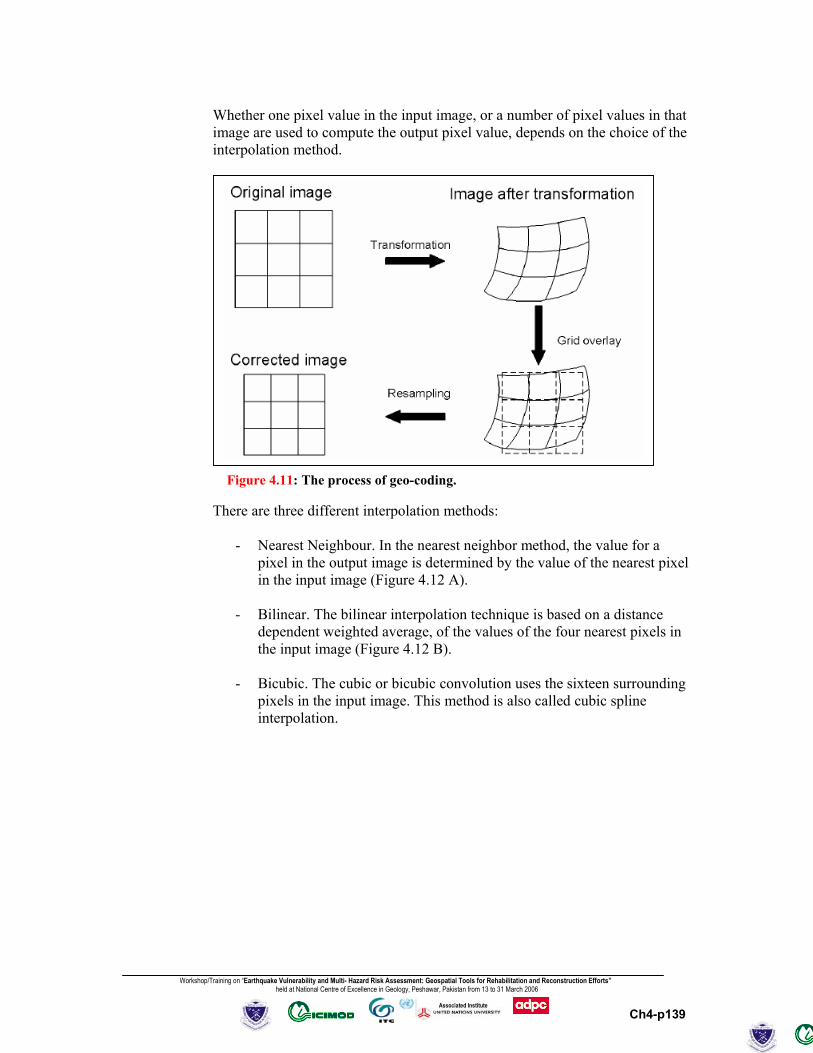
Workshop/Training on “Earthquake Vulnerability and Multi- Hazard Risk Assessment: Geospatial Tools for Rehabilitation and Reconstruction Efforts” held at National Centre of Excellence in Geology, Peshawar, Pakistan from 13 to 31 March 2006
Ch4-p139
Associated Institute
Whether one pixel value in the input image, or a number of pixel values in that image are used to compute the output pixel value, depends on the choice of the interpolation method. There are three different interpolation methods:
- Nearest Neighbour. In the nearest neighbor method, the value for a pixel in the output image is determined by the value of the nearest pixel in the input image (Figure 4.12 A).
- Bilinear. The bilinear interpolation technique is based on a distance
dependent weighted average, of the values of the four nearest pixels in the input image (Figure 4.12 B).
- Bicubic. The cubic or bicubic convolution uses the sixteen surrounding
pixels in the input image. This method is also called cubic spline interpolation.
Figure 4.11: The process of geo-coding.
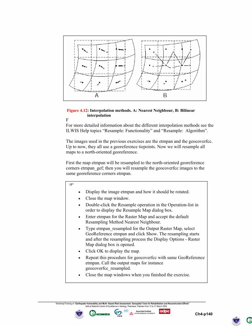
Workshop/Training on “Earthquake Vulnerability and Multi- Hazard Risk Assessment: Geospatial Tools for Rehabilitation and Reconstruction Efforts” held at National Centre of Excellence in Geology, Peshawar, Pakistan from 13 to 31 March 2006
Ch4-p140
Associated Institute
FFor more detailed information about the different interpolation methods see the ILWIS Help topics “Resample: Functionality” and “Resample: Algorithm”. The images used in the previous exercises are the etmpan and the geocoverfcc. Up to now, they all use a georeference tiepoints. Now we will resample all maps to a north-oriented georeference. First the map etmpan will be resampled to the north-oriented georeference corners etmpan_gef; then you will resample the geocoverfcc images to the same georeference corners etmpan.
• Display the image etmpan and how it should be rotated. • Close the map window. • Double-click the Resample operation in the Operation-list in
order to display the Resample Map dialog box. • Enter etmpan for the Raster Map and accept the default
Resampling Method Nearest Neighbour. • Type etmpan_resampled for the Output Raster Map, select
GeoReference etmpan and click Show. The resampling starts and after the resampling process the Display Options - Raster Map dialog box is opened.
• Click OK to display the map. • Repeat this procedure for geocoverfcc with same GeoReference
etmpan. Call the output maps for instance geocoverfcc_resampled.
• Close the map windows when you finished the exercise.
Figure 4.12: Interpolation methods. A: Nearest Neighbour, B: Bilinear interpolation
Workshop/Training on “Earthquake Vulnerability and Multi- Hazard Risk Assessment: Geospatial Tools for Rehabilitation and Reconstruction Efforts” held at National Centre of Excellence in Geology, Peshawar, Pakistan from 13 to 31 March 2006
Ch4-p141
Associated Institute
! What will happen to output pixel values if you use a bilinear or a bicubic interpolation during resampling? All the maps now have the same georeference etmpan and it is possible now to combine the maps with other digitized information of the area (that is rasterized on georeference etmpan as well).
Summary: Geometric corrections and image referencing
- Remote sensing data is affected by geometric distortions due to sensor
geometry, scanner and platform instabilities, earth rotation, earth curvature, etc.
- Remotely sensed images in raw format contain no reference to the
location of the data. In order to integrate these data with other data in a GIS, it is necessary to correct and adapt them geometrically, so that they have comparable resolution and projections as the other data sets.
- The geometric correction is executed by a transformation. The
transformation most frequently used to correct satellite images, is a first order transformation also called affine transformation.
- To define the transformation, it will be necessary to compute the
coefficients of the polynomials. For the computations, a number of points have to be selected that can be located accurately on the map (X,Y) and which are also identifiable in the image (row, column).
- The overall accuracy of the transformation is indicated by the average
of the errors in the reference points: The so-called Root Mean Square Error (RMSE) or Sigma.
- After geo-referencing, the image still has its original geometry and the
pixels have their initial position in the image, with respect to row and column indices.
- In case the image should be combined with data in another coordinate
system or with another georeference, a transformation has to be applied. This results in a “new” image where the pixels are stored in a new line/column geometry, which is related to the other georeference. This new image is created by means of resampling, by applying an interpolation method. The interpolation method is used to compute the radiometric values of the pixels, in the new image based on the DN values in the original image.
- After this action, the new image is called geo-coded and it can be
overlaid with data having the same coordinate system.
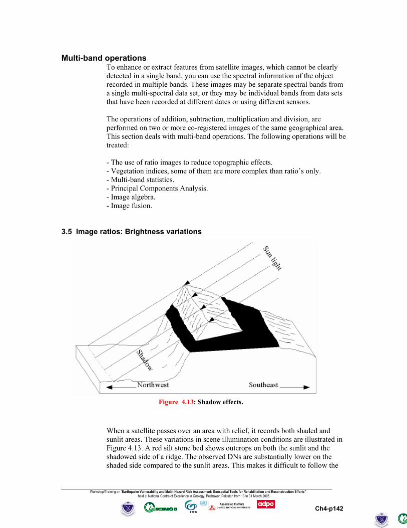
Workshop/Training on “Earthquake Vulnerability and Multi- Hazard Risk Assessment: Geospatial Tools for Rehabilitation and Reconstruction Efforts” held at National Centre of Excellence in Geology, Peshawar, Pakistan from 13 to 31 March 2006
Ch4-p142
Associated Institute
Multi-band operations To enhance or extract features from satellite images, which cannot be clearly detected in a single band, you can use the spectral information of the object recorded in multiple bands. These images may be separate spectral bands from a single multi-spectral data set, or they may be individual bands from data sets that have been recorded at different dates or using different sensors. The operations of addition, subtraction, multiplication and division, are performed on two or more co-registered images of the same geographical area. This section deals with multi-band operations. The following operations will be treated: - The use of ratio images to reduce topographic effects. - Vegetation indices, some of them are more complex than ratio’s only. - Multi-band statistics. - Principal Components Analysis. - Image algebra. - Image fusion.
3.5 Image ratios: Brightness variations
When a satellite passes over an area with relief, it records both shaded and sunlit areas. These variations in scene illumination conditions are illustrated in Figure 4.13. A red silt stone bed shows outcrops on both the sunlit and the shadowed side of a ridge. The observed DNs are substantially lower on the shaded side compared to the sunlit areas. This makes it difficult to follow the
Figure 4.13: Shadow effects.
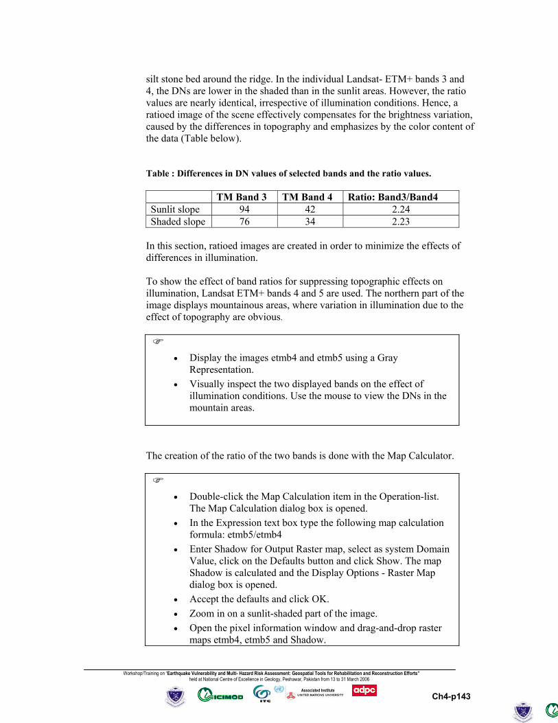
Workshop/Training on “Earthquake Vulnerability and Multi- Hazard Risk Assessment: Geospatial Tools for Rehabilitation and Reconstruction Efforts” held at National Centre of Excellence in Geology, Peshawar, Pakistan from 13 to 31 March 2006
Ch4-p143
Associated Institute
silt stone bed around the ridge. In the individual Landsat- ETM+ bands 3 and 4, the DNs are lower in the shaded than in the sunlit areas. However, the ratio values are nearly identical, irrespective of illumination conditions. Hence, a ratioed image of the scene effectively compensates for the brightness variation, caused by the differences in topography and emphasizes by the color content of the data (Table below). Table : Differences in DN values of selected bands and the ratio values.
TM Band 3 TM Band 4 Ratio: Band3/Band4 Sunlit slope 94 42 2.24 Shaded slope 76 34 2.23
In this section, ratioed images are created in order to minimize the effects of differences in illumination. To show the effect of band ratios for suppressing topographic effects on illumination, Landsat ETM+ bands 4 and 5 are used. The northern part of the image displays mountainous areas, where variation in illumination due to the effect of topography are obvious.
• Display the images etmb4 and etmb5 using a Gray
Representation. • Visually inspect the two displayed bands on the effect of
illumination conditions. Use the mouse to view the DNs in the mountain areas.
The creation of the ratio of the two bands is done with the Map Calculator.
• Double-click the Map Calculation item in the Operation-list.
The Map Calculation dialog box is opened. • In the Expression text box type the following map calculation
formula: etmb5/etmb4 • Enter Shadow for Output Raster map, select as system Domain
Value, click on the Defaults button and click Show. The map Shadow is calculated and the Display Options - Raster Map dialog box is opened.
• Accept the defaults and click OK. • Zoom in on a sunlit-shaded part of the image. • Open the pixel information window and drag-and-drop raster
maps etmb4, etmb5 and Shadow.
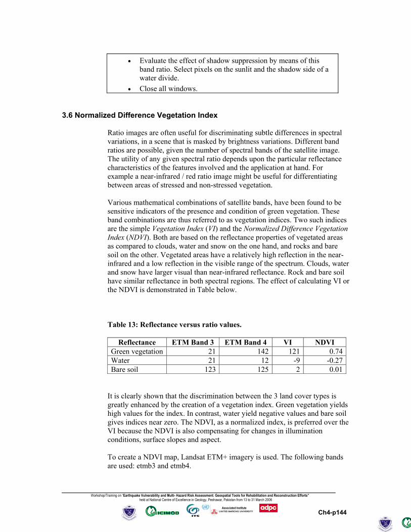
Workshop/Training on “Earthquake Vulnerability and Multi- Hazard Risk Assessment: Geospatial Tools for Rehabilitation and Reconstruction Efforts” held at National Centre of Excellence in Geology, Peshawar, Pakistan from 13 to 31 March 2006
Ch4-p144
Associated Institute
• Evaluate the effect of shadow suppression by means of this band ratio. Select pixels on the sunlit and the shadow side of a water divide.
• Close all windows.
3.6 Normalized Difference Vegetation Index
Ratio images are often useful for discriminating subtle differences in spectral variations, in a scene that is masked by brightness variations. Different band ratios are possible, given the number of spectral bands of the satellite image. The utility of any given spectral ratio depends upon the particular reflectance characteristics of the features involved and the application at hand. For example a near-infrared / red ratio image might be useful for differentiating between areas of stressed and non-stressed vegetation. Various mathematical combinations of satellite bands, have been found to be sensitive indicators of the presence and condition of green vegetation. These band combinations are thus referred to as vegetation indices. Two such indices are the simple Vegetation Index (VI) and the Normalized Difference Vegetation Index (NDVI). Both are based on the reflectance properties of vegetated areas as compared to clouds, water and snow on the one hand, and rocks and bare soil on the other. Vegetated areas have a relatively high reflection in the near-infrared and a low reflection in the visible range of the spectrum. Clouds, water and snow have larger visual than near-infrared reflectance. Rock and bare soil have similar reflectance in both spectral regions. The effect of calculating VI or the NDVI is demonstrated in Table below. Table 13: Reflectance versus ratio values.
Reflectance ETM Band 3 ETM Band 4 VI NDVI
Green vegetation 21 142 121 0.74Water 21 12 -9 -0.27Bare soil 123 125 2 0.01
It is clearly shown that the discrimination between the 3 land cover types is greatly enhanced by the creation of a vegetation index. Green vegetation yields high values for the index. In contrast, water yield negative values and bare soil gives indices near zero. The NDVI, as a normalized index, is preferred over the VI because the NDVI is also compensating for changes in illumination conditions, surface slopes and aspect. To create a NDVI map, Landsat ETM+ imagery is used. The following bands are used: etmb3 and etmb4.
Workshop/Training on “Earthquake Vulnerability and Multi- Hazard Risk Assessment: Geospatial Tools for Rehabilitation and Reconstruction Efforts” held at National Centre of Excellence in Geology, Peshawar, Pakistan from 13 to 31 March 2006
Ch4-p145
Associated Institute
The creation of the NDVI is done with the map calculator.
• Double-click the Map Calculation operation in the Operation-
list. The Map Calculation dialog box is opened. • In the Expression text box type the following map calculation
formula: (etmb4-etmb3)/(etmb4+etmb3) • Enter NDVI for Output Raster map, select system Domain
Value, change the Value Range to -1 and +1, and the Precision to 0.01.
• Click Show. The map NDVI is calculated and the Display Options – Raster Map dialog box is opened.
• In the Display Options - Raster Map dialog box select Pseudo as Representation. In this representation the colors range from blue (for the low DNs) through green (for the medium DNs) to red (for the high DNs). Click OK. The map NDVI is displayed.
• In the map window open the pixel information window and add the maps etmb3 and etmb4 to it.
• Move through the image with the mouse pointer and study the DN values of the input maps and how they are combined in the NDVI map.
• Before you create the NDVI image, first make sure that all bands are georeferenced.
• Close all windows after finishing the exercise.
! You can also use the NDVI function in MapCalc: NDVImap=NDVI(etmb4,etmb3)
3.7 Multi-band statistics The distribution of data values in a single band could be represented graphically using a histogram and mathematically by the variance statistics, which summarizes the differences between all the pixel values and the mean value of the channel (the range of data values in a channel is an indication of channel variability, it does not indicate the way the values are distributed between the minimum and maximum values). The correlation between two (or more) channels can be shown graphically by a scatter plot and mathematically by the covariance statistics. A scatter plot is a two dimensional graph, with on the horizontal axis the values of one channel, and on the vertical axis the values of the second channel. The points in the graph indicate the data or pixel values. The values in a covariance matrix indicate also the correlation:
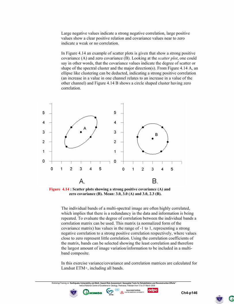
Workshop/Training on “Earthquake Vulnerability and Multi- Hazard Risk Assessment: Geospatial Tools for Rehabilitation and Reconstruction Efforts” held at National Centre of Excellence in Geology, Peshawar, Pakistan from 13 to 31 March 2006
Ch4-p146
Associated Institute
Large negative values indicate a strong negative correlation, large positive values show a clear positive relation and covariance values near to zero indicate a weak or no correlation. In Figure 4.14 an example of scatter plots is given that show a strong positive covariance (A) and zero covariance (B). Looking at the scatter plot, one could say in other words, that the covariance values indicate the degree of scatter or shape of the spectral cluster and the major direction(s). From Figure 4.14 A, an ellipse like clustering can be deducted, indicating a strong positive correlation (an increase in a value in one channel relates to an increase in a value of the other channel) and Figure 4.14 B shows a circle shaped cluster having zero correlation.
The individual bands of a multi-spectral image are often highly correlated, which implies that there is a redundancy in the data and information is being repeated. To evaluate the degree of correlation between the individual bands a correlation matrix can be used. This matrix (a normalized form of the covariance matrix) has values in the range of -1 to 1, representing a strong negative correlation to a strong positive correlation respectively, where values close to zero represent little correlation. Using the correlation coefficients of the matrix, bands can be selected showing the least correlation and therefore the largest amount of image variation/information to be included in a multi-band composite. In this exercise variance/covariance and correlation matrices are calculated for Landsat ETM+, including all bands.
Figure 4.14 : Scatter plots showing a strong positive covariance (A) and zero covariance (B). Mean: 3.0, 3.0 (A) and 3.0, 2.3 (B).
Workshop/Training on “Earthquake Vulnerability and Multi- Hazard Risk Assessment: Geospatial Tools for Rehabilitation and Reconstruction Efforts” held at National Centre of Excellence in Geology, Peshawar, Pakistan from 13 to 31 March 2006
Ch4-p147
Associated Institute
• Double-click the Correlation Matrix operation in the Operation-list. The Show Correlation Matrix dialog box is opened.
• Select etmb1to7 for the Map List name and click OK. The correlation, mean and standard deviation for these bands are calculated and presented in the Matrix viewer. Study the correlation matrix and answer the following questions:
1) Which band(s) in general show the least correlation and why? 2) Are the visible and the infrared bands highly correlated? 3) Select a band combination using three bands, showing most of the
information or in other words, those bands having the least correlation.
• Display the three bands with the least correlation and combine
them by constructing a color composite. • Close all windows/dialog boxes when you finished the exercise.
You can also have a look in the Properties of the map list. On the Additional Info tab, Optimum Index Factors are listed. Click the Help button for more information.
3.8 Principal components analysis Another method, called Principal Components Analysis (PCA), can be applied to compact the redundant data into fewer layers. Principal component analysis can be used to transform a set of image bands, as that the new layers (also called components) are not correlated with one another. Because of this, each component carries new information. The components are ordered in terms of the amount of variance explained, the first two or three components will carry most of the real information of the original data set, while the later components describe only the minor variations (sometimes only noise). Therefore, only by keeping the first few components most of the information is kept. These components can be used to generate an RGB color composite, in which component 1 is displayed in red and component 2 and 3 in green and blue respectively. Such an image contains more information than any combination of the three original spectral bands. To perform PCA, the axis of the spectral space are rotated, the new axis are parallel to the axis of the ellipse (Figure 4.15). The length and the direction of the widest transect of the ellipse are calculated. The transect which corresponds to the major (longest) axis of the ellipse, is called the first principal component of the data. The direction of the first principal component is the first eigenvector, and the variance is given by the first eigenvalue. A new axis of the
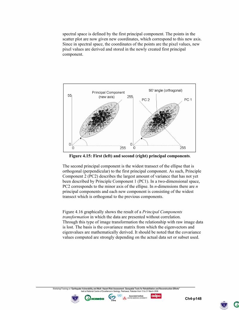
Workshop/Training on “Earthquake Vulnerability and Multi- Hazard Risk Assessment: Geospatial Tools for Rehabilitation and Reconstruction Efforts” held at National Centre of Excellence in Geology, Peshawar, Pakistan from 13 to 31 March 2006
Ch4-p148
Associated Institute
spectral space is defined by the first principal component. The points in the scatter plot are now given new coordinates, which correspond to this new axis. Since in spectral space, the coordinates of the points are the pixel values, new pixel values are derived and stored in the newly created first principal component.
Figure 4.15: First (left) and second (right) principal components. The second principal component is the widest transect of the ellipse that is orthogonal (perpendicular) to the first principal component. As such, Principle Component 2 (PC2) describes the largest amount of variance that has not yet been described by Principle Component 1 (PC1). In a two-dimensional space, PC2 corresponds to the minor axis of the ellipse. In n-dimensions there are n principal components and each new component is consisting of the widest transect which is orthogonal to the previous components. Figure 4.16 graphically shows the result of a Principal Components transformation in which the data are presented without correlation. Through this type of image transformation the relationship with raw image data is lost. The basis is the covariance matrix from which the eigenvectors and eigenvalues are mathematically derived. It should be noted that the covariance values computed are strongly depending on the actual data set or subset used.
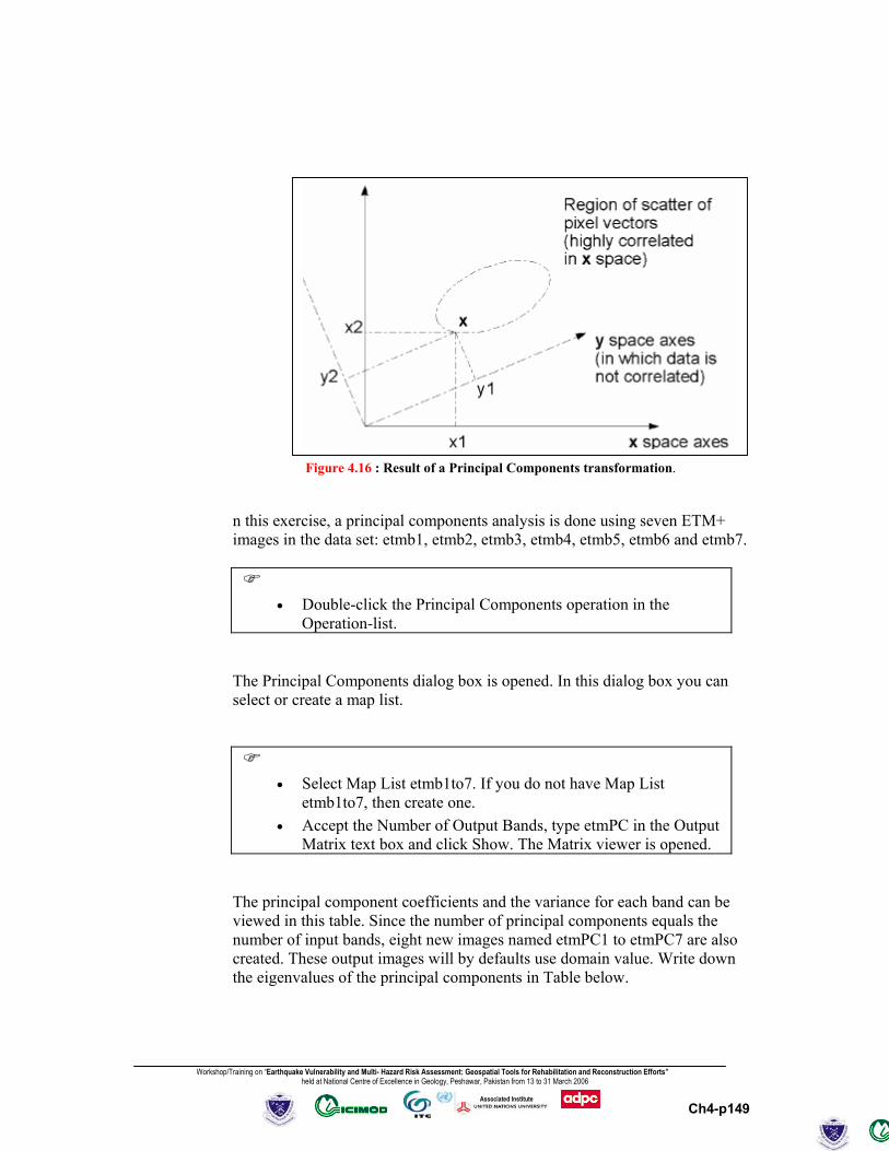
Workshop/Training on “Earthquake Vulnerability and Multi- Hazard Risk Assessment: Geospatial Tools for Rehabilitation and Reconstruction Efforts” held at National Centre of Excellence in Geology, Peshawar, Pakistan from 13 to 31 March 2006
Ch4-p149
Associated Institute
n this exercise, a principal components analysis is done using seven ETM+ images in the data set: etmb1, etmb2, etmb3, etmb4, etmb5, etmb6 and etmb7.
• Double-click the Principal Components operation in the
Operation-list. The Principal Components dialog box is opened. In this dialog box you can select or create a map list.
• Select Map List etmb1to7. If you do not have Map List
etmb1to7, then create one. • Accept the Number of Output Bands, type etmPC in the Output
Matrix text box and click Show. The Matrix viewer is opened. The principal component coefficients and the variance for each band can be viewed in this table. Since the number of principal components equals the number of input bands, eight new images named etmPC1 to etmPC7 are also created. These output images will by defaults use domain value. Write down the eigenvalues of the principal components in Table below.
Figure 4.16 : Result of a Principal Components transformation.

Workshop/Training on “Earthquake Vulnerability and Multi- Hazard Risk Assessment: Geospatial Tools for Rehabilitation and Reconstruction Efforts” held at National Centre of Excellence in Geology, Peshawar, Pakistan from 13 to 31 March 2006
Ch4-p150
Associated Institute
Table: Eigenvalues. etmb1 etmb2 etmb3 etmb4 etmb5 etmb6a etmb6b etmb7etmPC1 etmPC2 etmPC3 etmPC4 etmPC5 etmPC6 etmPC7 etmPC8
All ETM+ bands have a positive eigenvalue in principal component 1, therefore this PC mainly explains the intensity difference of the input bands. Explain the contribution of the ETM+ bands in principal components 2 and 3? Write down in the table below the variance explained per component. Table: Variance explained.
PC Variance % etmPC1 etmPC2 etmPC3 etmPC4 etmPC5 etmPC6 etmPC7 etmPC8
8

Workshop/Training on “Earthquake Vulnerability and Multi- Hazard Risk Assessment: Geospatial Tools for Rehabilitation and Reconstruction Efforts” held at National Centre of Excellence in Geology, Peshawar, Pakistan from 13 to 31 March 2006
Ch4-p151
Associated Institute
• Open the Properties of map etm PCl to check the expression of
the first axis: etm PC1= 0.212*etmb1 + 0.185*etmb2 + 0.201*etmb3 + 0.243*etmb4 + 0.244*etmb5 + 0.555*etmb6a + 0.649*etmb6b + 0.179*etmb7
• Double-click raster map etmPCl in the Catalog to calculate the first principal component.
• In the Display Options - Raster Map dialog box select Gray as Representation. Keep in mind the % of variance that is explained in this single image. Accept all other defaults and click OK.
• Open image etmPC2 and use again the Gray Representation. • Open the File menu in the map window and choose Properties,
select map etmPC2 and check the expression.
Compare the values in the expression with the eigenvalues noted in “Table EigenValues” above. Check whether your answer given to the question: “Explain the contribution of the ETM+ bands in principal components 2 and 3?” is correct?
• Calculate etmPC3.
A color composite can be created of the images produced by the principal component analysis. To create such a color composite, the domain type of the images should be changed from value to image.
• Create an interactive color composite using images etmPC1,
etmPC2 and etmPC3 for the Red, Green and Blue Bands respectively. Remember that the etmPC maps should be in a map list.
• Compare this color composite map with color composite etmmcc432 created in section 3.
• Close the map windows when you have finished the exercise.
Workshop/Training on “Earthquake Vulnerability and Multi- Hazard Risk Assessment: Geospatial Tools for Rehabilitation and Reconstruction Efforts” held at National Centre of Excellence in Geology, Peshawar, Pakistan from 13 to 31 March 2006
Ch4-p152
Associated Institute
3.9 Image arithmetics
Arithmetic operations are useful for calculating the average values and other purpose. The images have to be of same georefrence system and same pixel size. For expample: Average=(map1+map2)/2 Difference=map1-map2
3.10 Image fusion
Image fusion is the process of combining digital images, by modifying the data values, using a certain procedure. Before starting the fusion process the data should be properly co-registered. Combining for example both optical and microwave data, through image fusion techniques, results in a new data set. One of the fusion techniques has already been described: Principal Component Analysis (PCA). Another commonly used technique is the Red-Green-Blue transformation (RGB) into Intensity-Hue-Saturation (IHS), the intensity component is commonly replaced with another image and the modified data set is transformed back into the three primary colors. This technique is used to integrate for example a radar or panchromatic image with a multi spectral data set. This exercise makes use of the intensity component of the data sets used are Landsat ETM+ multispectral bands 1, 2, 3 , 4 , 5 and ETM+ Panchromatic are used of northern Pakistan area. Landsat ETM+ multispectral bands has a spatial resolution of 30 meters but resample to a 10 meter resolution. The ETM+ Panchromatic image, with an original resolution of 14.25 meter is also resampled to 15 meters. Both images have the same georeference. It is recommended to have the image of same season and year. If you do not have the resampled images of Landsat ETM+ and Landsat ETM+PAN images, then create resampled images of those images using Image Processing, Resample option using “l7etmpan_150036_2001oct_15m_” Georeference system with the output image names etmmss15m and etmpan15m
• Display raster maps etmmss15m and etmpan15m, using the
default display options. Position the map windows next to each other. Check the values of these two images and compare them.
Workshop/Training on “Earthquake Vulnerability and Multi- Hazard Risk Assessment: Geospatial Tools for Rehabilitation and Reconstruction Efforts” held at National Centre of Excellence in Geology, Peshawar, Pakistan from 13 to 31 March 2006
Ch4-p153
Associated Institute
What can be concluded when looking at the spatial resolution? As the images have the same georeference, the fusion can be achieved through a combined display of the two data sets in the form of a color composite.
• Create a map list by double-clicking New Map List in the
Operation-list. The Create Map List dialog box appears. • Type etmmsspan in the Map List box. Select the maps
etmmss15m1, etmmss15m2, etmmss15m3, etmmss15m4, etmmss15m5 and etmpan15m and press the > button to add the images to the map list. Click OK.
• Double-click map list etmmsspan in the Catalog to open it. • Click the Open As Color Composite button to open the Display
Options - Map List as ColorComp dialog box. • Select for the Red Band: etmpan15m, for the Green Band:
etmmss15m3 and for the Blue Band: etmmss15m4. Accept the other defaults and click OK to display the map.
• Check the result and close the map window afterwards.
In the next step, the data sets are fused by means of a replacement of the combined intensity of the three ETM+ multispectral bands, by the intensity of the ETM+ Panchromatic image. This results in a sharpening of the image due to the higher spatial resolution of the panchromatic image. The results are again displayed as a color composite.
• To calculate the combined intensity, type the following MapCalc formula on the Command line of the Main window: Intensity =( etmmss15m3 + etmmss15m4 + etmmss15m5)/3
• Make sure the Domain Image is selected in the Raster Map Definition dialog box and click Define.
• For the intensity replacement, enter the expressions given below, choose for each output map the Image Domain and accept the other defaults in the Raster Map Definition dialog boxes. Intensity1= etmmss15m3/Intensity* etmpan15m Intensity2= etmmss15m4/Intensity* etmpan15m Intensity3= etmmss15m5/Intensity* etmpan15m
• Create a map list Intensity, add the three intensity maps and show a color composite as follows: for Red Band: Intensity1; for Green Band: Intensity2; for Blue Band: Intensity3.

Workshop/Training on “Earthquake Vulnerability and Multi- Hazard Risk Assessment: Geospatial Tools for Rehabilitation and Reconstruction Efforts” held at National Centre of Excellence in Geology, Peshawar, Pakistan from 13 to 31 March 2006
Ch4-p154
Associated Institute
What can be concluded when the fused image is compared to the image created in the previous exercise?
• Close the map windows when you have finished the exercise.
Summary: Multi-band operations
- To enhance or extract features from satellite images, which cannot be clearly detected in a single band, you can use the spectral information of the object recorded in multiple bands.
- The operations of addition, subtraction, multiplication and division are
performed on two or more co-registered images of the same geographical area.
- Brightness variations: a ratioed image of the scene effectively
compensates for the brightness variation, caused by the differences in topography and emphasized by the color content of the data.
- Normalized Difference Vegetation Index (NDVI): Ratio images are
often useful for discriminating subtle differences in spectral variations, in a scene that is masked by brightness variations.
The utility of any given spectral ratio, depends upon the particular reflectance characteristics of the features involved and the application at hand.
- Various mathematical combinations of satellite bands, have been found to be sensitive indicators of the presence and condition of green vegetation. These band combinations are thus referred to as vegetation indices. Two such indices are the simple vegetation index (VI) and the normalized difference vegetation index (NDVI).
- The NDVI, as a normalized index, is preferred over the VI because the
NDVI is also compensating for changes in illumination conditions, surface slopes and aspect.
- Multi-band statistics
The distribution of data values in a single band could be mathematically represented by the variance statistics, which summarize the differences between all the pixel values and the mean value of the channel. The correlation between two (or more) channels can be mathematically shown by the covariance statistics. The values in a covariance matrix indicate also the correlation: Large negative values indicate a strong negative correlation, large positive values show a clear positive relation and covariance values near to zero indicate a weak or no correlation. The covariance values indicate the degree of scatter or shape of the
Workshop/Training on “Earthquake Vulnerability and Multi- Hazard Risk Assessment: Geospatial Tools for Rehabilitation and Reconstruction Efforts” held at National Centre of Excellence in Geology, Peshawar, Pakistan from 13 to 31 March 2006
Ch4-p155
Associated Institute
spectral cluster and the major direction(s). The individual bands of a multi-spectral image are often highly correlated, which implies that there is a redundancy in the data and information is being repeated. To evaluate the degree of correlation between the individual bands a correlation matrix can be used. This matrix (a normalized form of the covariance matrix) has values in the range of -1 to 1.
- Principal Components Analysis (PCA) can be applied to compact the
redundant data into fewer layers. Principal component analysis can be used to transform a set of image bands, as that the new layers are not correlated with one another. The first two or three components will carry most of the real information of the original data set. Therefore, only by keeping the first few components most of the information is kept. Through this type of image transformation the relationship with the raw image data is lost. It should be noted that the covariance values computed are strongly depending on the actual data set or subset used.
- Image fusion is the process of combining digital images, by modifying
the data values, using a certain procedure. Data sets are for example fused by means of a replacement of the combined intensity of the three TM bands, by the intensity of a panchromatic image.
Workshop/Training on “Earthquake Vulnerability and Multi- Hazard Risk Assessment: Geospatial Tools for Rehabilitation and Reconstruction Efforts” held at National Centre of Excellence in Geology, Peshawar, Pakistan from 13 to 31 March 2006
Ch4-p156
Associated Institute
3.11 Image classification Measured reflection values in an image depend on the local characteristics of the earth surface; in other words there is a relationship between land cover and measured reflection values. In order to extract information from the image data, this relationship must be found. The process to find the relationship is called classification. Classification can be done using a single band, in a process called density slicing, or using many bands (multi-spectral classification).
Density slicing In theory, it is possible to base a classification on a single spectral band of a remote sensing image, by means of single band classification or density slicing. Density slicing is a technique, whereby the DNs distributed along the horizontal axis of an image histogram, are divided into a series of user-specified intervals or slices. The number of slices and the boundaries between the slices depend on the different land covers in the area. All the DNs falling within a given interval in the input image are then displayed using a single class name in the output map. The image used in the exercise is a Landsat7 ETM+ band 4 of an area in northern Pakistan. Firstly, the ranges of the DN values representing the different land cover types have to be determined. Secondly, a domain group with the slice boundaries, names and codes has to be created.
• Display the image etmb4. • Move through the image and write down the values of water
and land. Fill in the data in Table below. Zoom in if necessary. Select also some mixed pixels along the land/water boundary.
Table: DN values per cover class of Landsat7 ETM+ Band 4.
Cover class DN values of Landsat7 ETM+ Band 4 Land Water
By a visual interpretation of the spectral reflectance of the cover classes in Landsat7 ETM+ Band 4, differences are observed with regard to their gray tones. Density slicing will only give reasonable results, if the DN values of the cover classes are not overlapping each other, as indicated in Figure 4.16.
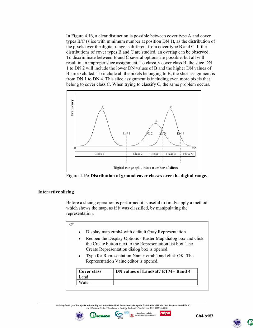
Workshop/Training on “Earthquake Vulnerability and Multi- Hazard Risk Assessment: Geospatial Tools for Rehabilitation and Reconstruction Efforts” held at National Centre of Excellence in Geology, Peshawar, Pakistan from 13 to 31 March 2006
Ch4-p157
Associated Institute
In Figure 4.16, a clear distinction is possible between cover type A and cover types B/C (slice with minimum number at position DN 1), as the distribution of the pixels over the digital range is different from cover type B and C. If the distributions of cover types B and C are studied, an overlap can be observed. To discriminate between B and C several options are possible, but all will result in an improper slice assignment. To classify cover class B, the slice DN 1 to DN 2 will include the lower DN values of B and the higher DN values of B are excluded. To include all the pixels belonging to B, the slice assignment is from DN 1 to DN 4. This slice assignment is including even more pixels that belong to cover class C. When trying to classify C, the same problem occurs. Figure 4.16: Distribution of ground cover classes over the digital range.
Interactive slicing
Before a slicing operation is performed it is useful to firstly apply a method which shows the map, as if it was classified, by manipulating the representation.
• Display map etmb4 with default Gray Representation. • Reopen the Display Options - Raster Map dialog box and click
the Create button next to the Representation list box. The Create Representation dialog box is opened.
• Type for Representation Name: etmb4 and click OK. The Representation Value editor is opened.
Cover class DN values of Landsat7 ETM+ Band 4 Land Water
Workshop/Training on “Earthquake Vulnerability and Multi- Hazard Risk Assessment: Geospatial Tools for Rehabilitation and Reconstruction Efforts” held at National Centre of Excellence in Geology, Peshawar, Pakistan from 13 to 31 March 2006
Ch4-p158
Associated Institute
• Open the Edit menu and select Insert Limit. The Insert Limit
dialog box is opened. Enter the limit you have written down in Table above to differentiate land from water, and select the color Blue.
• Insert also the other limit shown in the table and select the color Green for it.
• Open the list box, which appears after you click the word Stretch between the two limits. Select Upper. Do the same for the other.
• Click the Redraw button in the map window to see the map with the new representation.
• When satisfied, close the Representation Value editor.
The representation can thus be edited, and the result shown on the screen (by using the Redraw button in the map window). This allows you to interactively select the best boundaries for the classification.
Slicing operation
Now you will do the actual classification, using the Slicing operation.
• Double-click the Slicing operation in the Operation-list. The
Map Slicing dialog box is opened. • Select etmb4 in the Raster Map list box. • Type Slices in the Output Raster Map text box. • Type Classified etmb4 image in the Description text box. • Click the Create Domain button. The Create Domain dialog box
is opened. • Type Slices in the Domain Name text box. • Make sure that the Group check box is selected and accept all
other defaults by clicking the OK button. The Domain Group editor is opened.
For a group domain, you can enter an upper boundary, a name and a code for each class/group. This domain will be used to slice or classify the raster map etmb4.
Cover class DN values of Landsat7 ETM+ Band 4 Land Water

Workshop/Training on “Earthquake Vulnerability and Multi- Hazard Risk Assessment: Geospatial Tools for Rehabilitation and Reconstruction Efforts” held at National Centre of Excellence in Geology, Peshawar, Pakistan from 13 to 31 March 2006
Ch4-p159
Associated Institute
The upper boundaries and group names that you have entered in Table above will be used in this exercise.
• Click the button in the toolbar of the Domain Group editor. The Add Domain Item dialog box appears.
• Type the value from Table above in the Upper Bound text box. • Type Water in the Name text box. The use of a Code and a
Description is optional. It will not be used now. • Click OK. • Press the Insert key of the keyboard to enter the next upper
boundary and name.
• Press the Open Representation button in the toolbar. The Representation Class editor appears, showing the groups/classes that are present in the domain with different colors.
• Double-click a color box in the editor and select a pre-defined color, or create your own color.
• Exit the Representation Class editor when you are satisfied with the colors.
• Exit the Domain Group editor. • Click Show in the Slicing dialog box. The Display Options -
Raster Map dialog box is opened. • Accept the defaults by clicking OK. • In the map window open the pixel information window and
compare the values of the original map with the names in the classified map.
• Close the windows after finishing the exercise. When you create a domain group, a representation is also created. It is possible to edit the colors of the output groups/classes from the Domain Group editor, or by opening the representation in the Catalog. To edit the representation: If you are not satisfied with the results, perform the same procedure again with a new set of boundaries or by editing the existing slices.
Piece-wise linear stretching In the same way as described in the exercise on interactive slicing, you can also do a piece-wise linear stretching of images by creating a new representation.

Workshop/Training on “Earthquake Vulnerability and Multi- Hazard Risk Assessment: Geospatial Tools for Rehabilitation and Reconstruction Efforts” held at National Centre of Excellence in Geology, Peshawar, Pakistan from 13 to 31 March 2006
Ch4-p160
Associated Institute
While for interactive slicing, we used ‘upper’ boundary values (Figure 4.17 left) for piece-wise linear stretch, we will use the ‘stretch’ option between limits (Figure 4.17 right). The piece-wise linear contrast stretch is very similar to the linear contrast stretch, but the linear interpolation of the output values is applied between user-defined DN values. This method is useful to enhance a certain cover type, for example water.
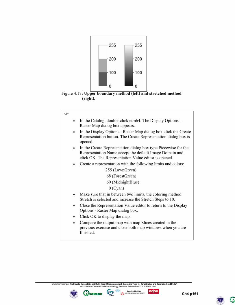
Workshop/Training on “Earthquake Vulnerability and Multi- Hazard Risk Assessment: Geospatial Tools for Rehabilitation and Reconstruction Efforts” held at National Centre of Excellence in Geology, Peshawar, Pakistan from 13 to 31 March 2006
Ch4-p161
Associated Institute
Figure 4.17: Upper boundary method (left) and stretched method (right).
• In the Catalog, double-click etmb4. The Display Options -
Raster Map dialog box appears. • In the Display Options - Raster Map dialog box click the Create
Representation button. The Create Representation dialog box is opened.
• In the Create Representation dialog box type Piecewise for the Representation Name accept the default Image Domain and click OK. The Representation Value editor is opened.
• Create a representation with the following limits and colors: 255 (LawnGreen) 68 (ForestGreen) 60 (MidnightBlue) 0 (Cyan)
• Make sure that in between two limits, the coloring method Stretch is selected and increase the Stretch Steps to 10.
• Close the Representation Value editor to return to the Display Options - Raster Map dialog box.
• Click OK to display the map. • Compare the output map with map Slices created in the
previous exercise and close both map windows when you are finished.
Workshop/Training on “Earthquake Vulnerability and Multi- Hazard Risk Assessment: Geospatial Tools for Rehabilitation and Reconstruction Efforts” held at National Centre of Excellence in Geology, Peshawar, Pakistan from 13 to 31 March 2006
Ch4-p162
Associated Institute
Multi-spectral image classification Multi-spectral image classification is used to extract thematic information from satellite images in a semi-automatic way. Different methods for image classification exist; some of them are based on the theory about probabilities. Looking at a certain image pixel in M bands simultaneously, M values are observed at the same time. Using multi-spectral Landsat7 ETM+ images, where M=7, seven reflection values per pixel are given. For instance, (34, 25, 117, 120, and so on) in one pixel, in another (34, 24, 119, 122, and so on) and in a third (11, 77, 51, 43, and so on). The values found for 1 pixel in several bands are called feature vectors. It can be recognized that the first two sets of values are quite similar and that the third is different from the other two. The first two probably belong to the same (land cover) class and the third one belongs to another class. In classification jargon it is common to call the three bands “features”. The term features instead of bands is used because it is very usual to apply transformations to the image, prior to classification. They are called “feature transformations” and their results are called “derived features”. Examples are: Principal Components, HIS transformations, etc. In one pixel, the values in the (three) features can be regarded as components of a 3- dimensional vector, the feature vector. Such a vector can be plotted in a 2- or 3- dimensional space called a feature space. Pixels which belong to the same (land cover) class and which have similar characteristics, end up near to each other in a feature space, regardless of how far they are from each other in the terrain and in the image. All pixels belonging to a certain class will (hopefully) form a cluster in the feature space. Moreover, it is hoped that other pixels, belonging to other classes, fall outside this cluster (but in other clusters, belonging to those other classes). A large number of classification methods exist. To make some order, the first distinction is between unsupervised and supervised classification. For satellite image applications, the second is generally considered more important. In order to make the classifier work with thematic (instead of spectral) classes, some “knowledge” about the relationship between classes and feature vectors must be given. Theoretically, this could be done from a database in which the relationships between (thematic) classes and feature vectors are stored. It is tempting to assume that in the past, enough images of each kind of sensor have been analyzed, as to know the spectral characteristics of all relevant classes. This would mean, for example, that a pixel with feature vector (44, 32, 81,121) in a multi-spectral etmb4 image always means grass, whereas (12, 56, 49,73) is always a forest pixel. Unfortunately, the observed feature vectors in a particular image are influenced by a large amount of other factors than land cover, such as atmospheric conditions, sun angle (as function of latitude, time of day, date and terrain

Workshop/Training on “Earthquake Vulnerability and Multi- Hazard Risk Assessment: Geospatial Tools for Rehabilitation and Reconstruction Efforts” held at National Centre of Excellence in Geology, Peshawar, Pakistan from 13 to 31 March 2006
Ch4-p163
Associated Institute
relief), soil types, soil humidity, growing stage of the vegetation, wind (affecting orientation of leafs), etc. The problems we meet when trying to take all these influences into account vary from ‘quite easy’ to ‘practically impossible’; at least, vast amounts of additional data (DEMs, soil maps, etc.) would be required.
Sampling Therefore, supervised classification methods are much more widely used. The process is divided into two phases: a training phase, where the user ’trains’ the computer, by assigning for a limited number of pixels to what classes they belong in this particular image, followed by the decision making phase, where the computer assigns a class label to all (other) image pixels, by looking for each pixel to which of the trained classes this pixel is most similar. During the training phase, the classes to be used are defined. About each class some “ground truth” is needed: a number of places in the image area that are known to belong to that class. This knowledge must have been acquired beforehand, for instance as a result of fieldwork, or from an existing map (assuming that in some areas the class membership has not changed since the map was produced). If the ground truth is available, training samples (small areas or individual pixels) are indicated in the image and the corresponding class names are entered. A sample set has to be created in which the relevant data regarding input bands (map list), cover classes (domain codes) and background image for selecting the training areas is stored. The map presented below is giving the ground truth information, as well as the cover classes to be used. The images used in this exercise are Landsat7 ETM+ multispectral images from the area of northern Pakistan: Landsat7 ETM+ band 1: etmb1 Landsat7 ETM+ band 2: etmb2 Landsat7 ETM+ band 3: etmb3 Landsat7 ETM+ band 4: etmb4 Landsat7 ETM+ band 5: etmb5 Landsat7 ETM+ band 6a: etmb6a Landsat7 ETM+ band 6b: etmb6b Landsat7 ETM+ band 7: etmb7 As the selection of the training areas is done on a color composite, it has to be created beforehand.
• Create a map list which contains the Landsat7 ETM+
multispectral bands. Display this as a color composite. Use etmb4 for Red, etmb3 for Green and etmb2 for Blue.
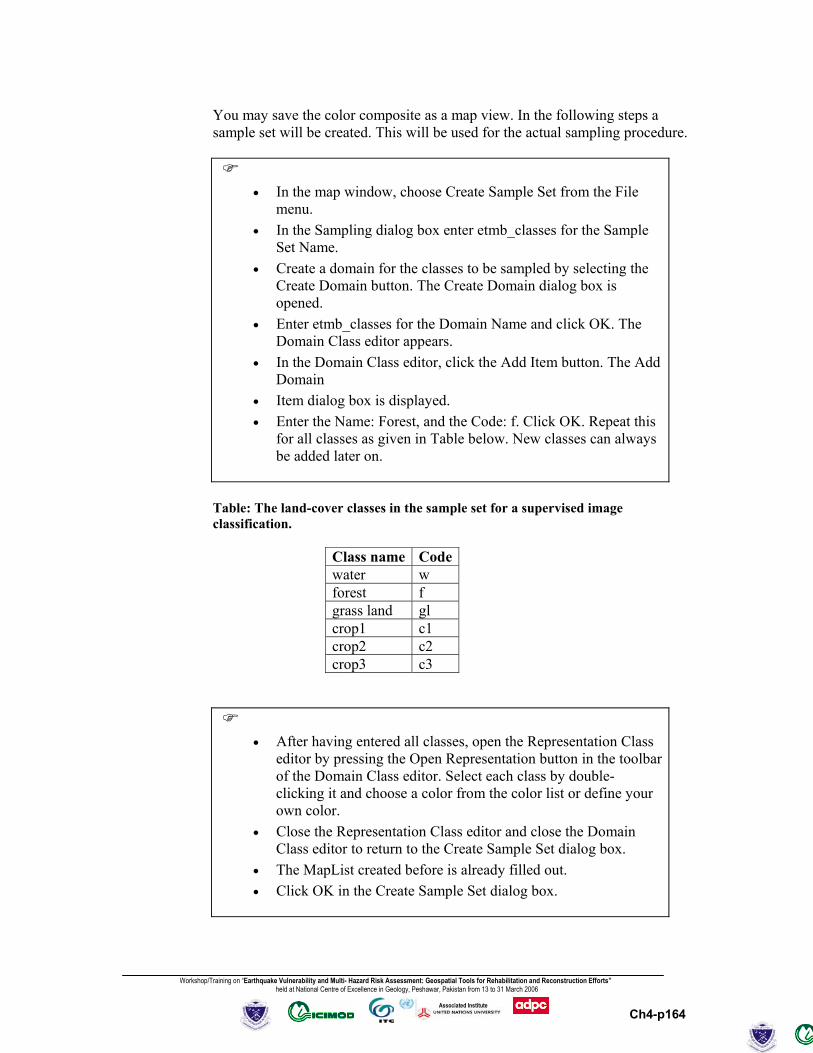
Workshop/Training on “Earthquake Vulnerability and Multi- Hazard Risk Assessment: Geospatial Tools for Rehabilitation and Reconstruction Efforts” held at National Centre of Excellence in Geology, Peshawar, Pakistan from 13 to 31 March 2006
Ch4-p164
Associated Institute
You may save the color composite as a map view. In the following steps a sample set will be created. This will be used for the actual sampling procedure.
• In the map window, choose Create Sample Set from the File
menu. • In the Sampling dialog box enter etmb_classes for the Sample
Set Name. • Create a domain for the classes to be sampled by selecting the
Create Domain button. The Create Domain dialog box is opened.
• Enter etmb_classes for the Domain Name and click OK. The Domain Class editor appears.
• In the Domain Class editor, click the Add Item button. The Add Domain
• Item dialog box is displayed. • Enter the Name: Forest, and the Code: f. Click OK. Repeat this
for all classes as given in Table below. New classes can always be added later on.
Table: The land-cover classes in the sample set for a supervised image classification.
Class name Codewater w forest f grass land gl crop1 c1 crop2 c2 crop3 c3
• After having entered all classes, open the Representation Class
editor by pressing the Open Representation button in the toolbar of the Domain Class editor. Select each class by double-clicking it and choose a color from the color list or define your own color.
• Close the Representation Class editor and close the Domain Class editor to return to the Create Sample Set dialog box.
• The MapList created before is already filled out. • Click OK in the Create Sample Set dialog box.

Workshop/Training on “Earthquake Vulnerability and Multi- Hazard Risk Assessment: Geospatial Tools for Rehabilitation and Reconstruction Efforts” held at National Centre of Excellence in Geology, Peshawar, Pakistan from 13 to 31 March 2006
Ch4-p165
Associated Institute
The Sample Set editor will be started. Two windows are displayed: A map window showing the false color composite and a window showing the sample set statistics. During the sampling procedure, consult also available reference maps of northern Pakistan.
• Zoom in on an area with water and press the Normal button in
the toolbar to return to the normal mode. To select pixels press the left mouse button and drag the cursor. When the mouse button is released, the statistics of the current selection of pixels are shown in the Sample Statistics window, Current Selection (Figure 4.18).
• Click the right mouse button to reveal the context-sensitive menu and select Edit. Select the appropriate class from the class list (w: Water). Once this selection is added to the class, the total class statistics are shown in the upper part of the table.
• One can always compare the statistics of a sample with the statistics of a class, by selecting the class in the class list.
• Repeat the sampling procedure for a number of water samples and then continue with sampling the other land cover classes.
• If a land cover class has not yet been defined and, therefore, does not appear in the class list, a new class can be created by selecting <new>.
• Add a new class (Name: Clean Glacier, Code: cg). Take samples of this class.
! To select multiple training pixels you can drag rectangles or you can hold the Ctrl-key.
The Sample Statistics window contains the code and name of the selected class as well as the number of bands. The following statistics are shown for a selected class (see Figure 4.18):
- Mean value of pixels (Mean). - Standard deviation of pixels (StDev). - The number of pixels having the predominant value (Nr). - The predominant pixel value (Pred.). - The total number of the selected pixels (Total).
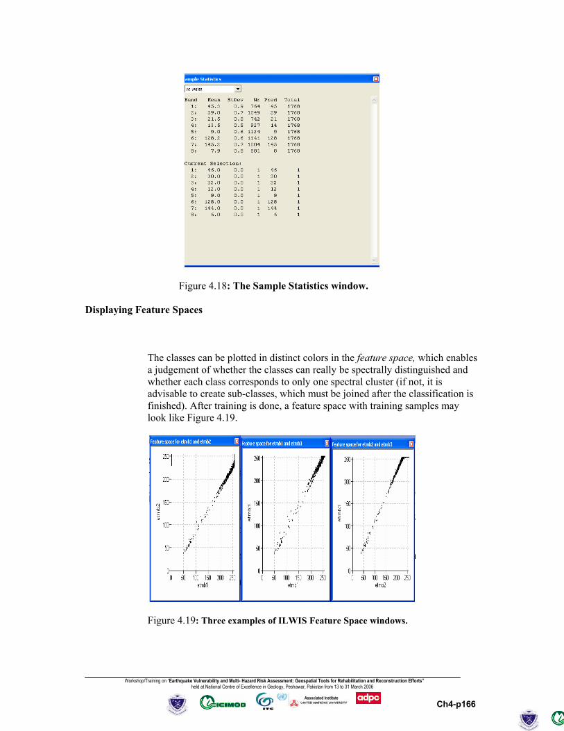
Workshop/Training on “Earthquake Vulnerability and Multi- Hazard Risk Assessment: Geospatial Tools for Rehabilitation and Reconstruction Efforts” held at National Centre of Excellence in Geology, Peshawar, Pakistan from 13 to 31 March 2006
Ch4-p166
Associated Institute
Figure 4.18: The Sample Statistics window. Displaying Feature Spaces
The classes can be plotted in distinct colors in the feature space, which enables a judgement of whether the classes can really be spectrally distinguished and whether each class corresponds to only one spectral cluster (if not, it is advisable to create sub-classes, which must be joined after the classification is finished). After training is done, a feature space with training samples may look like Figure 4.19.
Figure 4.19: Three examples of ILWIS Feature Space windows.

Workshop/Training on “Earthquake Vulnerability and Multi- Hazard Risk Assessment: Geospatial Tools for Rehabilitation and Reconstruction Efforts” held at National Centre of Excellence in Geology, Peshawar, Pakistan from 13 to 31 March 2006
Ch4-p167
Associated Institute
The number of training samples should be between 30 and some hundreds of samples per class, depending on the number of features and on the decision making that is going to be applied. The feature space is a graph in which DN values of one band are plotted against the values of another. To view a feature space:
• Click the Feature Space button in the toolbar of the Sample Set editor. The Feature Space dialog box is opened.
• Select two bands for which a feature space should be created. Select etmb1 for the horizontal axis (band 1) and etmb2 for the vertical axis (band 2). Click OK. The feature space of etmb1 against etmb2 is displayed.
• Try also the other band combinations for the feature space display.
You will probably see some overlapping classes in the feature space. What can be said about the standard deviation for the clean glacier area and how can this be explained?
• After you have finished the sampling, close all windows and return to the ILWIS Main window.
Classification
It is the task of the decision-making algorithm to make a partitioning of the feature space, according to our training samples. For every possible feature vector in the feature space, the program must decide to which of the sets of training pixels this feature vector is most similar. After that, the program makes an output map where each image pixel is assigned a class label, according to the feature space partitioning. Some algorithms are able to decide that feature vectors in certain parts of the feature space are not similar to any of the trained classes. They assign to those image pixels the class label “Unknown”. In case the area indeed contains classes that were not included in the training phase, the result “unknown” is probably more realistic than to make a “wild” guess. To find the relationship between classes and feature vectors is not as trivial as it may seem. Therefore, various decision-making algorithms are being used; they are different in the way they partition the feature space. Four of them are:

Workshop/Training on “Earthquake Vulnerability and Multi- Hazard Risk Assessment: Geospatial Tools for Rehabilitation and Reconstruction Efforts” held at National Centre of Excellence in Geology, Peshawar, Pakistan from 13 to 31 March 2006
Ch4-p168
Associated Institute
- The Box classifier is the simplest classification method: In 2-D space, rectangles are created around the training feature vector for each class; in 3-D they are actually boxes (blocks). The position and sizes of the boxes can be ‘exactly around’ the feature vectors (Min-Max method), or according to the mean vector (this will be at the center of a box) and the standard deviations of the feature vector, calculated separately per feature (this determines the size of the box in that dimension). In both cases, the user is allowed to change the sizes by entering a “multiplication factor”. In parts of the feature space where boxes overlap, it is usual to give priority to the smallest box. Feature vectors in the image that fall outside all boxes will be “unknown”. - The Minimum Distance-to-mean classifier, first calculates for each class the mean vector of the training feature vectors. Then, the feature space is partitioned by giving to each feature vector the class label of the nearest mean vector, according to Euclidean metric. Usually it is possible to specify a maximum distance threshold: if the nearest mean is still further away than that threshold, it is assumed that none of the classes is similar enough and the result will be “unknown”. - Minimum Mahalanobis Distance classifier. For the spectral values of a pixel to be classified, the distances towards the class means are calculated as Mahalanobis distance. The Mahalanobis distance depends on the distances towards class means and the variance-covariance matrix of each class. The class name with the shortest Mahalanobis distance is assigned, if this distance is smaller than the user-defined threshold value. Else, the undefined value is assigned. - Gaussian Maximum Likelihood classifiers assume that the feature vectors of each class are (statistically) distributed according to a “multivariate normal probability density function”. The training samples are used to estimate the parameters of the distributions. The boundaries between the different partitions in the feature space are placed where the decision changes from one class to another. They are called decision boundaries. In this exercise, different types of land-cover in the area will be detected by implementing a supervised classification, using the sample set prepared in the previous exercise on sampling. The output will be a map with domain type class representing land-cover units in the area. The four standard techniques for classifying an image in ILWIS are: 1) The Box classifier; 2) The Minimum Distance classifier; 3) The Mahalanobis Distance classifier, and 4) The Maximum Likelihood classifier. Each classifier uses a sample set, only the procedure to classify an image is different.
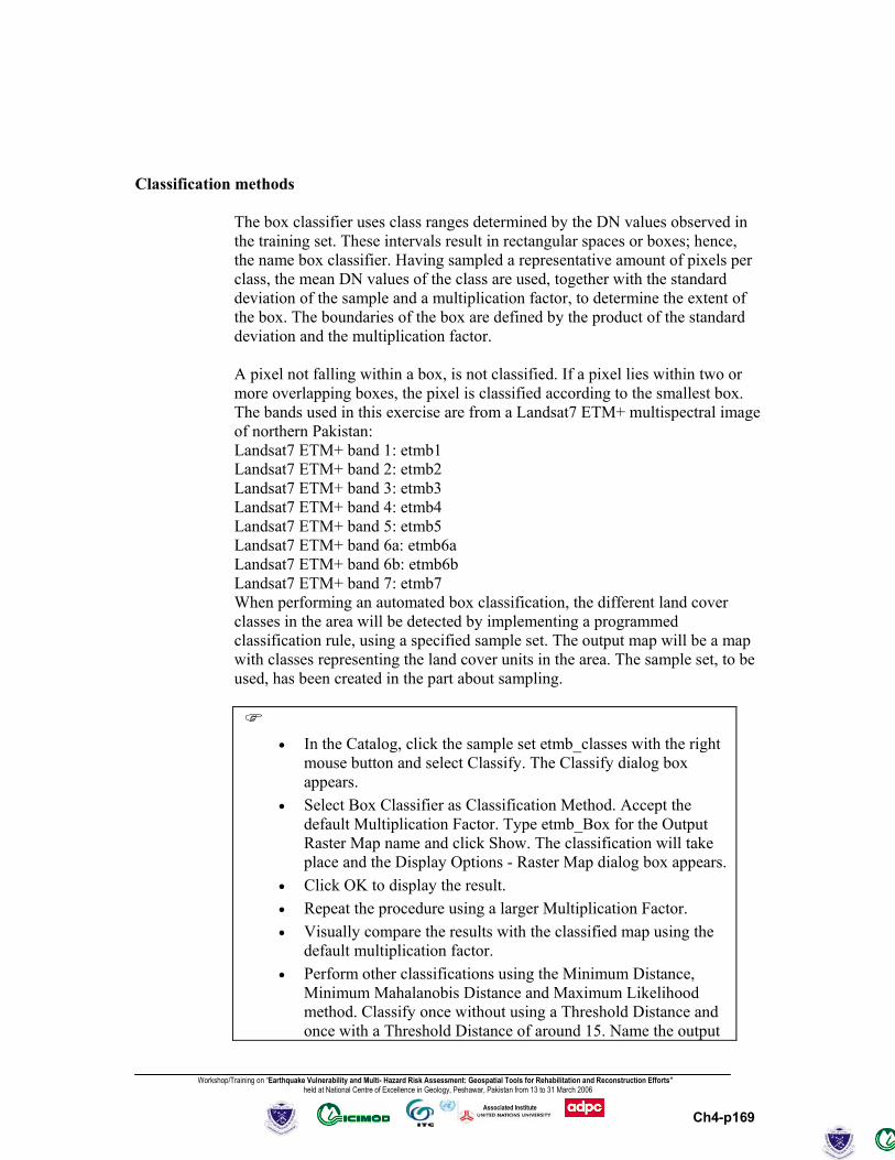
Workshop/Training on “Earthquake Vulnerability and Multi- Hazard Risk Assessment: Geospatial Tools for Rehabilitation and Reconstruction Efforts” held at National Centre of Excellence in Geology, Peshawar, Pakistan from 13 to 31 March 2006
Ch4-p169
Associated Institute
Classification methods
The box classifier uses class ranges determined by the DN values observed in the training set. These intervals result in rectangular spaces or boxes; hence, the name box classifier. Having sampled a representative amount of pixels per class, the mean DN values of the class are used, together with the standard deviation of the sample and a multiplication factor, to determine the extent of the box. The boundaries of the box are defined by the product of the standard deviation and the multiplication factor. A pixel not falling within a box, is not classified. If a pixel lies within two or more overlapping boxes, the pixel is classified according to the smallest box. The bands used in this exercise are from a Landsat7 ETM+ multispectral image of northern Pakistan: Landsat7 ETM+ band 1: etmb1 Landsat7 ETM+ band 2: etmb2 Landsat7 ETM+ band 3: etmb3 Landsat7 ETM+ band 4: etmb4 Landsat7 ETM+ band 5: etmb5 Landsat7 ETM+ band 6a: etmb6a Landsat7 ETM+ band 6b: etmb6b Landsat7 ETM+ band 7: etmb7 When performing an automated box classification, the different land cover classes in the area will be detected by implementing a programmed classification rule, using a specified sample set. The output map will be a map with classes representing the land cover units in the area. The sample set, to be used, has been created in the part about sampling.
• In the Catalog, click the sample set etmb_classes with the right mouse button and select Classify. The Classify dialog box appears.
• Select Box Classifier as Classification Method. Accept the default Multiplication Factor. Type etmb_Box for the Output Raster Map name and click Show. The classification will take place and the Display Options - Raster Map dialog box appears.
• Click OK to display the result. • Repeat the procedure using a larger Multiplication Factor. • Visually compare the results with the classified map using the
default multiplication factor. • Perform other classifications using the Minimum Distance,
Minimum Mahalanobis Distance and Maximum Likelihood method. Classify once without using a Threshold Distance and once with a Threshold Distance of around 15. Name the output

Workshop/Training on “Earthquake Vulnerability and Multi- Hazard Risk Assessment: Geospatial Tools for Rehabilitation and Reconstruction Efforts” held at National Centre of Excellence in Geology, Peshawar, Pakistan from 13 to 31 March 2006
Ch4-p170
Associated Institute
images for instance etmb_MinDist, etmb_MinMahaDist and etmb_MaxLikehd.
• Compare the results with the box classified maps. • Close all map windows when you have finished the exercise.
Evaluate the reclassified results
The final result is compared with the original values in bands of Landsat7 ETM+ multispectral images. For the complex and more homogenous land covers the results can be compared with the original bands.
• Display the land-cover map based on Landsat7 ETM+ of 2001 April 30 with thirteen landcover classes prepared by USGS downloaded from EDC as used in first exercise “landcover13lclasses”. Make sure that it is georeferenced.
• Check this also for the Landsat7 ETM+ multispectral bands. • Open the pixel information window and add the maps etmb1,
etmb2, etmb3, etmb4, etmb5 etmb6a, etmb6b, etmb7, and etmb_Box.
• Evaluate for pixels the different cover classes defined and the result of your classification.
• Close the map window and the pixel information window.
To get a better idea of the overall accuracy of the classification, use has to be made of the test set which contains additional ground truth data, which have not been used to train the classifier. Crossing the test set with the classified image and creation of a confusion matrix, is an established method to assess the accuracy of a classification. ! See the ILWIS Help topic How to calculate a confusion matrix for more information about creating a confusion matrix. It is not recommended to use the same sample map for both the classification and the accuracy assessment, because this will produce figures that are too optimistic.
Post classification operations The final classification may not meet the expected results. This can be due to spectral overlap in the sample set, or because the classifier has not been trained properly. If this is the case the classification process should be repeated, incorporating for example more spectral classes. Defining sub-classes, when a bi-model distribution or large standard deviation/variance exists in a class, will
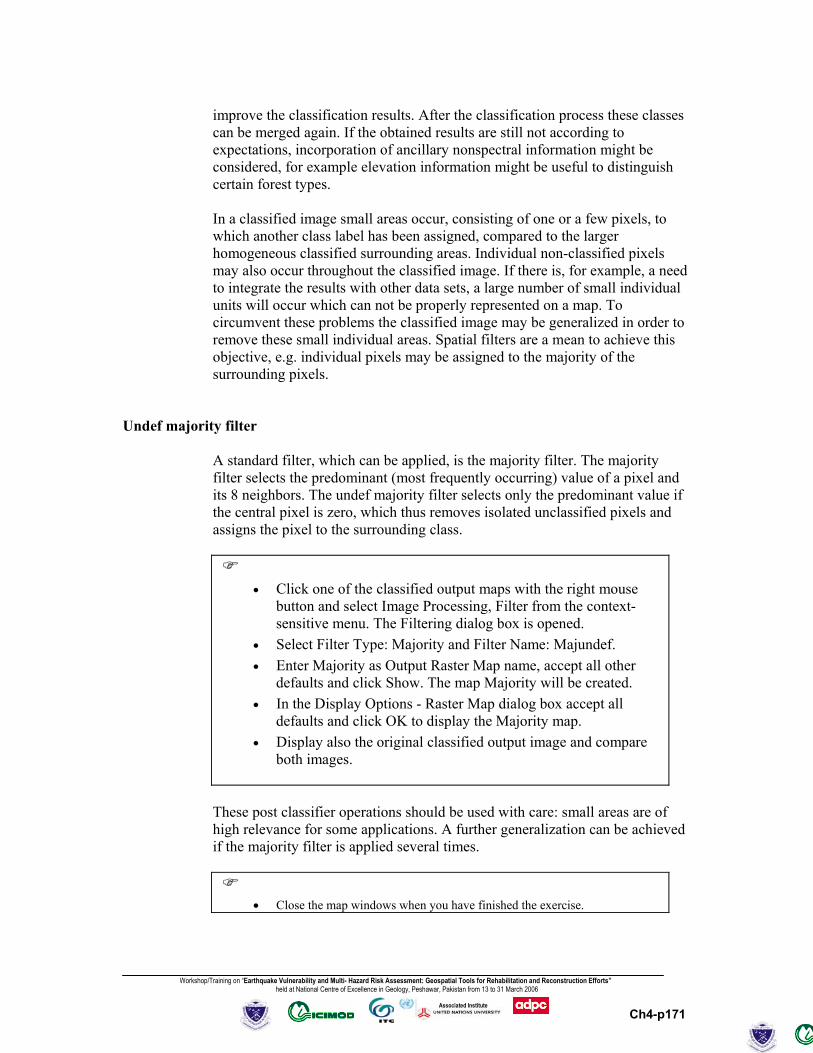
Workshop/Training on “Earthquake Vulnerability and Multi- Hazard Risk Assessment: Geospatial Tools for Rehabilitation and Reconstruction Efforts” held at National Centre of Excellence in Geology, Peshawar, Pakistan from 13 to 31 March 2006
Ch4-p171
Associated Institute
improve the classification results. After the classification process these classes can be merged again. If the obtained results are still not according to expectations, incorporation of ancillary nonspectral information might be considered, for example elevation information might be useful to distinguish certain forest types. In a classified image small areas occur, consisting of one or a few pixels, to which another class label has been assigned, compared to the larger homogeneous classified surrounding areas. Individual non-classified pixels may also occur throughout the classified image. If there is, for example, a need to integrate the results with other data sets, a large number of small individual units will occur which can not be properly represented on a map. To circumvent these problems the classified image may be generalized in order to remove these small individual areas. Spatial filters are a mean to achieve this objective, e.g. individual pixels may be assigned to the majority of the surrounding pixels.
Undef majority filter
A standard filter, which can be applied, is the majority filter. The majority filter selects the predominant (most frequently occurring) value of a pixel and its 8 neighbors. The undef majority filter selects only the predominant value if the central pixel is zero, which thus removes isolated unclassified pixels and assigns the pixel to the surrounding class.
• Click one of the classified output maps with the right mouse button and select Image Processing, Filter from the context-sensitive menu. The Filtering dialog box is opened.
• Select Filter Type: Majority and Filter Name: Majundef. • Enter Majority as Output Raster Map name, accept all other
defaults and click Show. The map Majority will be created. • In the Display Options - Raster Map dialog box accept all
defaults and click OK to display the Majority map. • Display also the original classified output image and compare
both images.
These post classifier operations should be used with care: small areas are of high relevance for some applications. A further generalization can be achieved if the majority filter is applied several times.
• Close the map windows when you have finished the exercise.
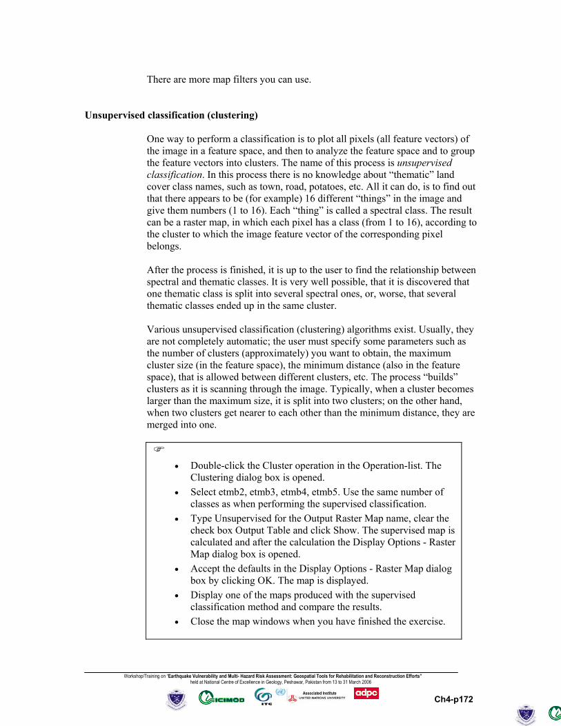
Workshop/Training on “Earthquake Vulnerability and Multi- Hazard Risk Assessment: Geospatial Tools for Rehabilitation and Reconstruction Efforts” held at National Centre of Excellence in Geology, Peshawar, Pakistan from 13 to 31 March 2006
Ch4-p172
Associated Institute
There are more map filters you can use.
Unsupervised classification (clustering)
One way to perform a classification is to plot all pixels (all feature vectors) of the image in a feature space, and then to analyze the feature space and to group the feature vectors into clusters. The name of this process is unsupervised classification. In this process there is no knowledge about “thematic” land cover class names, such as town, road, potatoes, etc. All it can do, is to find out that there appears to be (for example) 16 different “things” in the image and give them numbers (1 to 16). Each “thing” is called a spectral class. The result can be a raster map, in which each pixel has a class (from 1 to 16), according to the cluster to which the image feature vector of the corresponding pixel belongs. After the process is finished, it is up to the user to find the relationship between spectral and thematic classes. It is very well possible, that it is discovered that one thematic class is split into several spectral ones, or, worse, that several thematic classes ended up in the same cluster. Various unsupervised classification (clustering) algorithms exist. Usually, they are not completely automatic; the user must specify some parameters such as the number of clusters (approximately) you want to obtain, the maximum cluster size (in the feature space), the minimum distance (also in the feature space), that is allowed between different clusters, etc. The process “builds” clusters as it is scanning through the image. Typically, when a cluster becomes larger than the maximum size, it is split into two clusters; on the other hand, when two clusters get nearer to each other than the minimum distance, they are merged into one.
• Double-click the Cluster operation in the Operation-list. The Clustering dialog box is opened.
• Select etmb2, etmb3, etmb4, etmb5. Use the same number of classes as when performing the supervised classification.
• Type Unsupervised for the Output Raster Map name, clear the check box Output Table and click Show. The supervised map is calculated and after the calculation the Display Options - Raster Map dialog box is opened.
• Accept the defaults in the Display Options - Raster Map dialog box by clicking OK. The map is displayed.
• Display one of the maps produced with the supervised classification method and compare the results.
• Close the map windows when you have finished the exercise.
Workshop/Training on “Earthquake Vulnerability and Multi- Hazard Risk Assessment: Geospatial Tools for Rehabilitation and Reconstruction Efforts” held at National Centre of Excellence in Geology, Peshawar, Pakistan from 13 to 31 March 2006
Ch4-p173
Associated Institute
Summary: Image classification
- In order to extract information from the satellite images, the relationship between pixel values and land cover types must be found. The process to find the relationship is called classification.
- Density slicing is a technique, whereby the DNs distributed along the
horizontal axis of an image histogram, are divided into a series of user-specified intervals or slices. Density slicing will only give reasonable results, if the DN values of the cover classes are not overlapping each other.
- Multi spectral image classification is used to extract thematic
information from satellite images in a semi-automatic way. The values of the various bands found for 1 pixel in several bands are called feature vectors. Such a vector can be plotted in a 3-dimensional space, called feature space. Pixels belonging to the same (land cover) class and having similar characteristics, end up near to each other in the feature space. In order to make the classifier work with thematic (instead ofspectral) classes, some “knowledge” about the relationship between classes and feature vectors must be given.
- The classification process is divided into two phases: a training phase,
where the user “trains” the computer, by assigning for a limited number of pixels to what classes they belong in this particular image, followed by the decision making phase, where the computer assigns a class label to all (other) image pixels, by looking for each pixel to which of the trained classes this pixel is most similar.
- About each class some “ground truth” is needed: a number of places in
the image area that are known to belong to that class. It is the task of the decision- making algorithm to make a partitioning of the feature space, according to our training samples. For every possible feature vector in the feature space, the program must decide to which of the sets of training pixels this feature vector is most similar. After that, the program makes an output map where each image pixel is assigned a class label, according to the feature space partitioning.
- Various decision making algorithms are used: box classifier, minimum
distance to mean classifier, minimum Mahalanobis distance classifier and Gaussian maximum likelihood classifier.
- Unsupervised classification. One way to perform a classification is to
plot all pixels (all feature vectors) of the image in a feature space, and then to analyze the feature space and to group the feature vectors into clusters. In this process there is no knowledge about “thematic” land cover class names. The user must specify some parameters such as the number of clusters (approximately) you want to obtain, the maximum

Workshop/Training on “Earthquake Vulnerability and Multi- Hazard Risk Assessment: Geospatial Tools for Rehabilitation and Reconstruction Efforts” held at National Centre of Excellence in Geology, Peshawar, Pakistan from 13 to 31 March 2006
Ch4-p174
Associated Institute
cluster size (in the feature space), the minimum distance (also in the feature space), that is allowed between different clusters, etc.
________________________________________________________________________ The first step in the image processing after importing or downloading the image is geo-referencing. Only after geo-referencing, you should continue to other required steps in image processing. You can try the multi-band operation, such as Band Ratioing or Indices, Principal Component, Data Fusion, Multi-spectral classification, etc.