Chapter 4 Global symmetries in particle physics - UPMCzuber/Cours/chap4_12e.pdfGlobal symmetries in...

Chapter 4

Global symmetries in particle physics

Particle physics o↵ers a wonderful playground to illustrate the various manifestations of symme-

tries in physics. We will be only concerned in this chapter and the following one with “internal

symmetries”, excluding space-time symmetries.

We shall examine in turn various types of symmetries and their realizations, as exact sym-

metries, or broken explicitly, spontaneously or by quantum anomalies.

4.1 Global exact or broken symmetries. Spontaneous

breaking

4.1.1 Overview. Exact or broken symmetries

Transformations that concern us in this chapter are global symmetries and we discuss them in

the framework of (classical or quantum) field theory. A group G acts on degrees of freedom

of each field �(x) in the same way at all points x of space-time. For example, G acts on � by

a linear representation, and to each element g of the group corresponds a matrix or operator

D(g), independent of the point x

�(x) 7! D(g)�(x) . (4.1)

In a quantum theory, according to Wigner theorem, one assumes that this transformation is

also realized on vector-states of the Hilbert space of the theory by a unitary operator U(g),

and, as an operator, �(x) 7! U(g)�(x)U †(x).

This transformation may be a symmetry of dynamics, in which case U(g) commutes with

the Hamiltonian of the system, or in the Lagrangian picture, it leaves the Lagrangian invariant

and gives rise to Noether currents jµi of vanishing divergence (see Chapitre 01) and to conserved

1Here and below in this chapter, Chapitre 0 refers to Chap. 0 of the French version, especially in its discussionof Noether’s currents.

November 20, 2012 J.-B. Z M2 ICFP/Physique Theorique 2012

132 Chap.4. Global symmetries in particle physics

charges Qi =R

dx j0(x, t), i = 1, · · · , dim G. These charges act on fields as infinitesimal gener-

ators, classically in the sense of the Poisson bracket, {Qi,�(x)}�↵i = ��(x), and if everything

goes right in the quantum theory, as operators in the Hilbert space with commutation relations

with the fields [Qi,�(x)]�↵i = �i~��(x) and between themselves [Qi, Qj] = iC kij Qk. An im-

portant question will be indeed to know if a symmetry which is manifest at the classical level,

say on the Lagrangian, is actually realized in the quantum theory.

• An example of exact symmetry is provided by the U(1) invariance associated with electric

charge conservation. A field carrying an electric charge q (times |e|) is a complex field, it

transforms under the action of the group U(1) according to the irreducible representation

labelled by the integer q

�(x) 7! eiq↵�(x) ; �†(x) 7! e�iq↵�†(x) ,

and there is invariance (of the Lagrangian) if all fields transform that way, with a Noether cur-

rent jµ(x), sum of contributions of the di↵erent charged fields, being divergence-less, @µjµ(x) =

0, and the associated charge Q =P

qi is conserved. The quantum theory is quantum elec-

trodynamics, and there one proves that the classical U(1) symmetry, the current conservation

(and gauge invariance) are preserved by quantization and in particular by renormalization, for

example that all electric charges renormalize in the same way, see the course of Quantum Field

Theory.

Other invariances and conservation laws of a similar nature are those associated with bary-

onic or leptonic charges, which are conserved (until further notice . . . ).

• A symmetry may also be broken explicitely. For example the Lagrangian contains terms that

are non invariant under the action of G. In that case, the Noether currents are non conserved,

but their divergence reads

@µjµi (x) =

@L(x)

@↵i, (4.2)

(see Chapitre 0, § 4.2). We will see below with flavor SU(3) an example of a broken (or

“approximate”) symmetry.Certain types of breakings, called “soft”, are such that the symmetry is restored at short distance or high

energy. This is for example the case of scale invariance (by space dilatations), broken by the presence of any massscale in the theory, but restored –in a fairly subtle way– at short distance, see the study of the RenormalizationGroup in the courses of quantum or statistical field theory.

• A more subtle mechanism of symmetry breaking is that of spontaneous symmetry break-

ing. This refers to situations where the ground state of the system does not have a symmetry

apparent on the Lagrangian or on the equations of motion. The simplest illustration of this phe-

nomenon is provided by a classical system with one degree of freedom, described by the “double

well potential” of Fig. 4.1(a). Although the potential exhibits a manifest Z2 symmetry under

x ! �x, the system chooses a ground state in one of the two minima of the potential, which

breaks symmetry. This mechanism plays a fundamental role in physics, with diverse manifes-

tations ranging from condensed matter –ferromagnetism, superfluidity, supraconductivity. . . –

to particle physics –chiral symmetry, Higgs phenomenon– and cosmology.

J.-B. Z M2 ICFP/Physique Theorique 2012 November 20, 2012

§ 4.1. Global exact or broken symmetries. Spontaneous breaking 133

(a)

x

V(x)

a!a

x

V(x)

(b)

Figure 4.1: Potentials (a) with a “double well” ; (b) “mexican hat”

. Example. Spontaneous breaking in the O(n) model

The Lagrangian of the bosonic (and Minkovskian, here) “O(n) model” for a real n-component

field �� = {�i}L =

1

2(@��)2 � 1

2m2��2 � �

4(��2)2 (4.3)

is invariant under the O(n) rotation group. The Noether current jaµ = @µ�i(T a)ij�j (with T a real

antisymmetric) has a vanishing divergence, which implies the conservation of a “charge” etc.

The minimum of the potential corresponds to the ground state, alias the vacuum, of the theory.

If the parameter m2 is taken negative, the minimum of the potential V = 12m2��2 + �

4(��2)2 is

no longer at ��2 = 0 but at some value v2 of ��2 such that �m2 = �v2, see Fig. 4.1(b). The field

� “chooses” spontaneously a direction n (n2 = 1) in the internal space, in which its vacuum

expectation value (“vev” in the jargon) is non vanishing

h 0|��|0 i = vn . (4.4)

This “vev” breaks the initial invariance group G = O(n) down to its subgroup H that leaves

invariant the vector h 0|��|0 i = vn, hence a group isomorphic to O(n � 1). The fact that a

vacuum expectation value of a non invariant field be non zero, h 0|��|0 i 6= 0, signals that the

vacuum is not invariant : this is a case of spontaneous symmetry breaking. This is the mechanism

at work in a low temperature ferromagnet, for example, in which the non zero magnetization

signals the spontaneous breaking of the space rotation symmetry.

Exercise (see F. David’s course) : Set �� = (v +�)n+⇡⇡⇡, where ⇡⇡⇡ denote the n� 1 components

of the field �� orthogonal to h�� i = vn and determine the terms of V (�,⇡⇡⇡) that are linear and

quadratic in the fields � and ⇡⇡⇡ ; check that the linear term in � vanishes (minimum of the

potential), that � has a non-zero mass term, but that the ⇡⇡⇡ are massless, they are the Nambu–

Goldstone bosons of the spontaneously broken symmetry. This is a general phenomenon:

any continuous spontaneously broken symmetry is accompanied by the appearance of massless

excitations whose number equals that of the generators of the broken symmetry (Goldstone

theorem). More precisely when a group G is spontaneously broken into a subgroup H (group

of residual symmetry, invariance group of the ground state), a number d(G)�d(H) of massless

Goldstone bosons appears. In the previous example, G = O(n), H = O(n� 1), d(G)� d(H) =



n� 1.Let us give a simple proof of that theorem in the case of a Lagrangian field theory. We write L = 1

2

(@�)2�V (�) with quite generic notations, � denotes a set of fields {�i} on which acts a continuous transformationgroup G. The potential V is assumed to be invariant under the action infinitesimal transformations �a�i,a = 1, · · · ,dim G. For example for linear transformations: �a�i = T a

ij�j . We thus have

@V (�(x))@�i(x)

�a�i(x) = 0 .

Di↵erentiate this equation with respect to �j(x) (omitting everywhere the argument x)

@V

@�i

@�a�i

@�j+

@2V

@�i@�j�a�i = 0

and evaluate it at �(x) = v, a (constant, x-independent) minimum of the potential : the first term vanishes,the second tells us

@2V

@�i@�j

�

�

�

�=v�avi = 0 , (4.5)

where we write (with a little abuse of notation) �avi = �a�i|�=v. On the other hand, the theory is quantizednear that minimum v (“vacuum” of the theory) by writing �(x) = v + '(x) and by expanding

V (�) = V (v) +12

@2V

@�i@�j

�

�

�

�=v'i'j + · · ·

and the masses of the fields ' are then read o↵ the quadratic form. But (4.5) tells us that the “mass matrix”@2V

@�i@�j|�=v has as many “zero modes” (eigenvectors of vanishing eigenvalue) as there are independent variations

�avi 6= 0. If H is the invariance group of v, �avi 6= 0 for the generators of G that are not generators of H, andthere are indeed dim G� dim H massless modes, qed.

4.1.2 Chiral symmetry breaking

Consider a Lagrangian that involves massless fermions

L = i/@ + g( �µ )( �µ ) , (4.6)

where = { ↵}↵=1,··· ,N is a N -component vector of 4-spinor fields. Note the absence of a mass

term in (4.6). That Lagrangian is invariant under the action of two types of infinitesimal

transformations

�A (x) = �A (x) (4.7)

�B (x) = �B�5 (x) ,

where the matrices A and B are infinitesimal N ⇥ N antihermitian, that act on the “flavor”

indices ↵ but on spinor indices and hence commute with � matrices. Recall that �5 is Hermitian

and anticommutes with the �µ and check that �A = � �A, �B = �B�5. The conserved

Noether currents are respectively

Jaµ = T a�µ Ja(5)

µ = T a�5�µ , (4.8)

with T a infinitesimal generators of the unitary group U(N). The transformations of the first line

are called “vector”, those of the second, which involve �5, are “axial”. One may also rephrase it


§ 4.1. Global exact or broken symmetries. Spontaneous breaking 135

in terms of independent transformations of L := 12(I��5) and of R := 1

2(I+�5) ; one recalls

that (�5)2 = I and that 12(I ± �5) are thus projectors; one has thus L = †L�0 = 1

2 (I + �5),

etc, and

L = Li/@ L + Ri/@ R + g( L�µ L + R�µ R)( L�µ L + R�

µ R)

which is clearly invariant under the finite unitary transformations L ! U1 L, R ! U2 R,

with U1, U2 2 U(N). The group of chiral symmetry is thus U(N)⇥ U(N).

If we now introduce a mass term �L = �m (which “couples” the left and right compo-

nents L and R: �L = �m( R L + L R)), the “vector” symmetry is preserved, but the axial

one is not and gives rise to a divergence

@µJa(5)µ (x) / m T a�5 . (4.9)

The residual symmetry group is U(N), “diagonal” subgroup of U(N)⇥U(N) (diagonal in the

sense that one takes U1 = U2 in the transformations of L,R.)

The axial symmetry may also be spontaneously broken. Let us start from a Lagrangian,

sum of terms of the type (4.6) with N = 2 and (4.3) for n = 4, with a coupling term between

the fermions and the four bosons, traditionally denoted � and ⇡⇡⇡

L = �

i/@ + g(� + i⇡⇡⇡.⌧⌧⌧�5)�

+1

2

�

(@⇡⇡⇡)2 + (@�)2�� 1

2m2(�2 + ⇡⇡⇡2)� �

4(�2 + ⇡⇡⇡2)2 , (4.10)

in which the Pauli matrices have been exceptionally denoted by ⌧⌧⌧ not to confuse them with

the field �. The symmetry group is U(2)⇥U(2), with fields L, R and � + i⇡⇡⇡.⌧⌧⌧ transforming

respectively by the representations (12, 0), (0, 1

2) and (1

2, 1

2) of SU(2) ⇥ SU(2) (see exercise A).

If m2 < 0, the field � = (�,⇡⇡⇡) develops a non-zero vev, that may be oriented in the direction

� if one has initially introduced a small explicit breaking term �L = c�, the analogue of a

small magnetic field, which is then turned o↵. The vev is given as above by v = �m2/�, and,

rewriting �(x) = �0(x)+v, where the field �0 has now a vanishing vev, one sees that the fermions

have acquired a mass m = �gv, whereas the ⇡⇡⇡ are massless. This Lagrangian, the �-model of

Gell-Mann–Levy, has been proposed as a model explaining the chiral symmetry breaking and

the low mass of the ⇡ mesons, regarded as “quasi Nambu–Goldstone quasi-bosons” (“quasi” in

the sense that the chiral symmetry is only approximate before being spontaneously broken).

Some elements of that model will reappear in the standard model.

4.1.3 Quantum symmetry breaking. Anomalies

Another mode of symmetry breaking, of purely quantum nature, manifests itself in anomalies of quantum fieldtheories. A symmetry, which is apparent at the classical level of the Lagrangian, is broken by the e↵ect of“quantum corrections”. This is for instance what takes place with some chiral symmetries of the type juststudied: an axial current which is classically divergenceless may acquire by a “one-loop e↵ect” a divergence@µJµ

5

6= 0. If the “anomalous” current is the Noether current of an internal classical symmetry, that symmetryis broken by the quantum anomaly, which may cause interesting physical e↵ects (see discussion of the decay⇡0 ! ��, for example in [IZ] chap 11). But in a theory like a gauge theory where the conservation of the axialcurrent is crucial to ensure consistency –renormalizability, unitarity–, the anomaly constitutes a potential threatthat must be controlled. This is what happens in the standard model, and we return to it in Chap. 5. Anotherexample is provided by dilatation (scale) invariance of a massless theory, see the study of the renormalizationgroup in F. David’s course.



4.2 The SU(3) flavor symmetry and the quark model.

An important approximate symmetry is the “flavor” SU(3) symmetry, to which we devote the

rest of this chapter.

4.2.1 Why SU(3) ?

We saw (Chap. 0) that if the weak and electromagnetic interactions are neglected, hadrons,

i.e. particules subject to strong interactions such as proton and neutron, ⇡ mesons etc, fall into

“multiplets” of a SU(2) group of isospin. Or said di↵erently, the Hamiltonian (or Lagrangian)

of strong interactions is invariant under the action of that SU(2) group and consequently, the

SU(2) group is represented in the space of hadronic states by unitary representations. Proton

and neutron belong to a representation of dimension 2 and of isospin 12, the three pions ⇡±, ⇡0

form a representation of dimension 3 and isospin 1, etc. The electric charge Q of each of these

particles is related to the eigenvalue of the third component Iz of isospin by

Q =1

2B + Iz [for SU(2)] (4.11)

where a new quantum number B appears, the baryonic charge, supposed to be (additively)

conserved in all interactions (until further notice). B is 0 for ⇡ mesons, 1 for “baryons” as

proton or neutron, �1 for their antiparticles, 4 for an ↵ particle (Helium nucleus), etc.

This relation between Q and Iz must be amended for a new family of mesons (K±, K0, K0, · · · )and baryons ⇤0,⌃,⌅, . . . discovered at the end of the fifties. One assigns them a new quantum

number S, strangeness. This strangeness is assumed to be additively conserved in strong inter-

actions. Thus, if S is�1 for the ⇤0 and +1 for the K+ and the K0, the reaction p+⇡� ! ⇤0+K0

conserves strangeness, whereas the observed decay ⇤0 ! p+⇡� violates that conservation law,

as it proceeds through weak interactions. Relation (4.11) must be modified into the Gell-Mann–

Nishima relation

Q =1

2B +

1

2S + Iz =

1

2Y + Iz , (4.12)

where we introduced the hypercharge Y , which, at this stage, equals Y = B + S.

These conservation laws and di↵erent properties of mesons and baryons discovered then, in

particular their organisation into “octets”, led at the beginning of the sixties M. Gell-Mann

and Y. Ne’eman to postulate the existence of a group SU(3) of approximate symmetry of

strong interactions. The quantum numbers Iz and Y that are conserved and simultaneously

mesurable are interpreted as eigenvalues of two commuting charges, hence of two elements of a

Cartan algebra of rank 2, and the algebra of SU(3) is the natural candidate, as it possesses an

irreducible 8-dimensional representation (see also exercise C of Chap. 3).

In the defining representation 3 of SU(3), one constructs a basis of the Lie algebra su(3),

made of 8 Hermitian matrices �a that play the role of Pauli matrices �i for su(2). These

matrices are normalised by

tr�a�b = 2�ab . (4.13)


§ 4.2. The SU(3) flavor symmetry and the quark model. 137

I z I z

1 1

Y

0

KK

! ""

KK

! +

1 1

2

!1

+0

0!

Y

0

KK

##

KK

0! +

1 1

2

!1

*+*0

*0*!

0#"

0$

!1!1

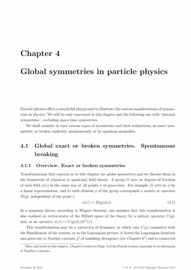
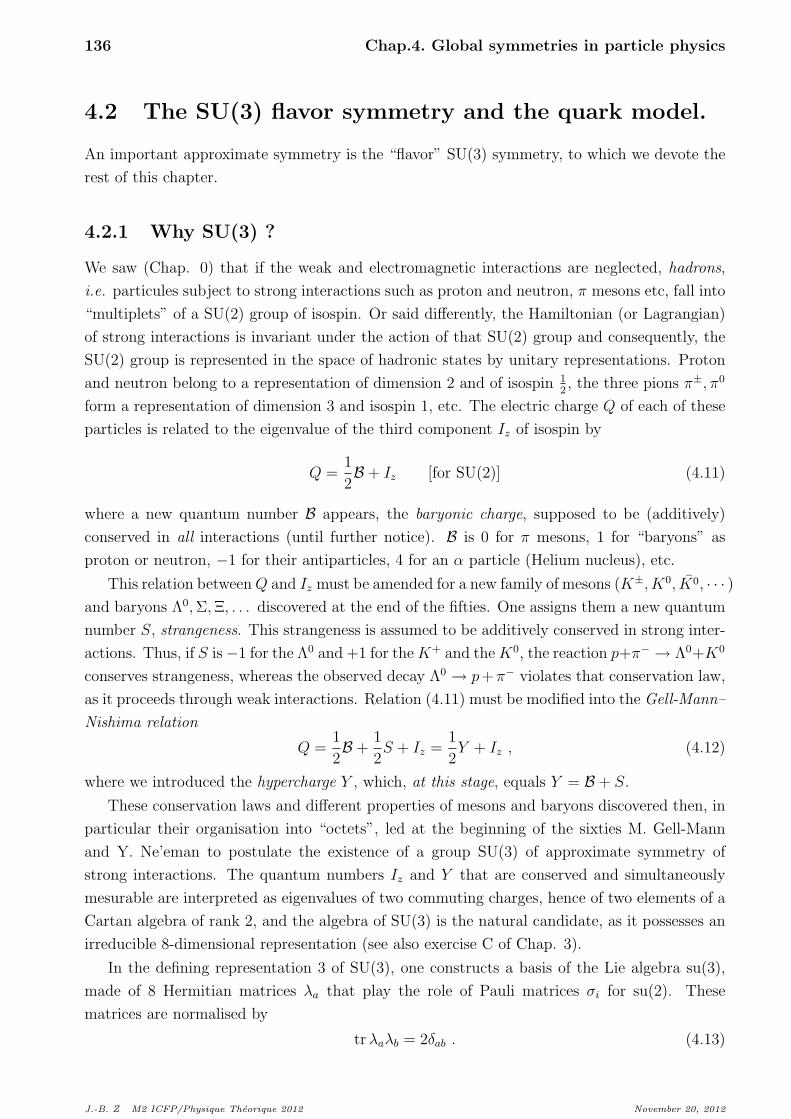
Figure 4.2: Octets of pseudoscalar (JP = 0�) and of vector mesons (JP = 1�)

!1

z

I z

!0 !+

!0!"

!"

"

+++0"

21 1 3

2!1

Y

I

Y

0

pn

# ##

$$! 0

0! +

1 1

2

!1

0%0

1

!1

1

&

'' ''

$$

###

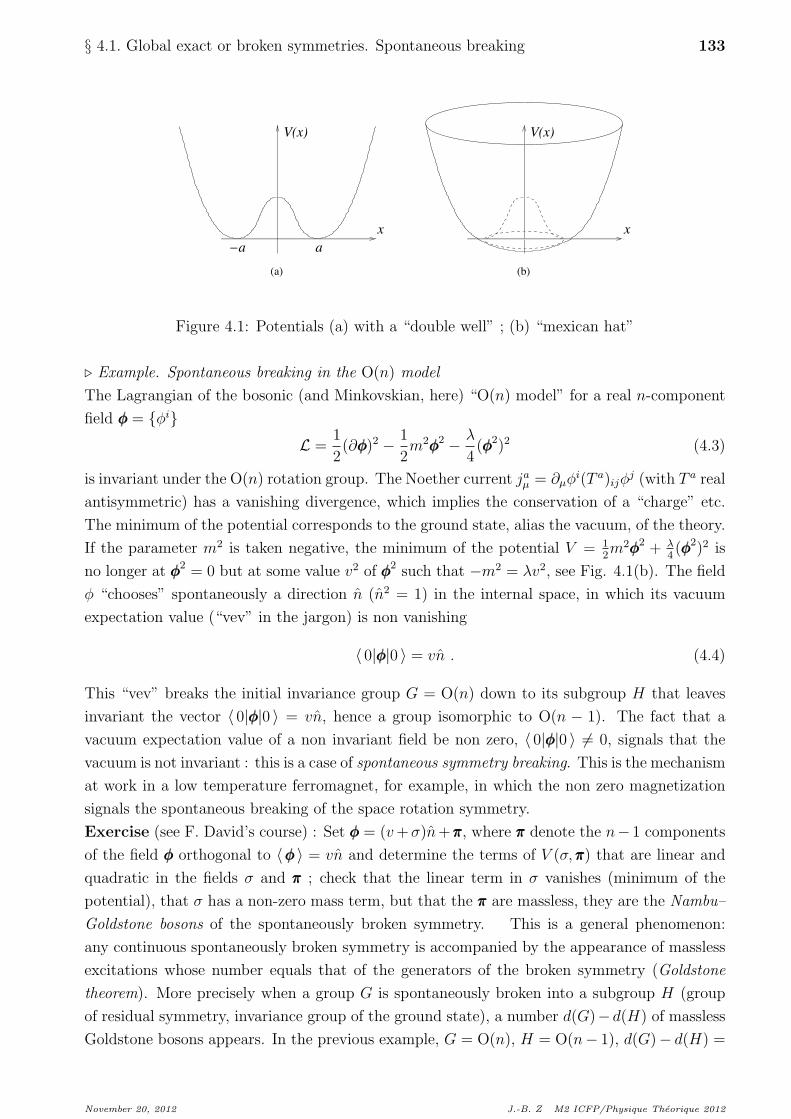
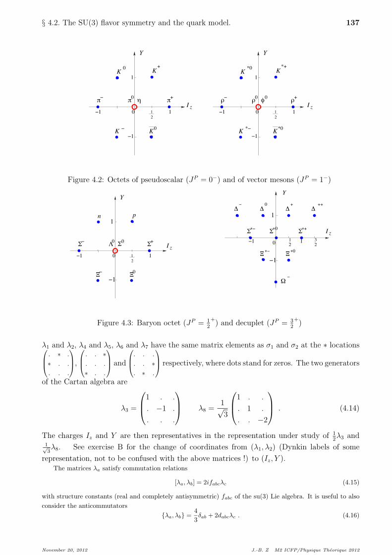
Figure 4.3: Baryon octet (JP = 12

+) and decuplet (JP = 3

2

+)

�1 and �2, �4 and �5, �6 and �7 have the same matrix elements as �1 and �2 at the ⇤ locations0

B

@

. ⇤ .

⇤ . .

. . .

1

C

A

,

0

B

@

. . ⇤

. . .

⇤ . .

1

C

A

and

0

B

@

. . .

. . ⇤

. ⇤ .

1

C

A

respectively, where dots stand for zeros. The two generators

of the Cartan algebra are

�3 =

0

B

@

1 . .

. �1 .

. . .

1

C

A

�8 =1p3

0

B

@

1 . .

. 1 .

. . �2

1

C

A

. (4.14)

The charges Iz and Y are then representatives in the representation under study of 12�3 and

1p3�8. See exercise B for the change of coordinates from (�1,�2) (Dynkin labels of some

representation, not to be confused with the above matrices !) to (Iz, Y ).The matrices �a satisfy commutation relations

[�a, �b] = 2ifabc�c (4.15)

with structure constants (real and completely antisymmetric) fabc of the su(3) Lie algebra. It is useful to alsoconsider the anticommutators

{�a, �b} =43�ab + 2dabc�c . (4.16)



Thanks to (4.13), (4.15) and (4.16) may be rewritten as tr ([�a, �b]�c) = 4ifabc, tr ({�a, �b}�c) = 4dabc. Thesenumbers f and d are tabulated in the literature . . . but they are easily computable ! Beware that in contrastwith (4.15), relation (4.16) and the (real, completely symmetric) constants dabc are proper to the 3-dimensionalrepresentation.

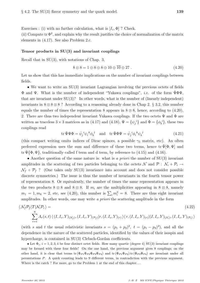
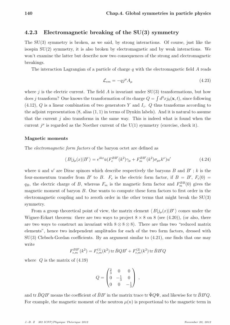
Hadrons are then organized in SU(3) representations. Each multiplet gathers particles with

the same spin J and parity P . For instance two octets of mesons with JP equal to 0� or 1� and

one octet and one “decuplet” of baryons of baryonic charge B = 1 are easily identified. Contrary

to isospin symmetry, the SU(3) symmetry 2 is not an exact symmetry of strong interactions.

The conservation laws and selection rules that follow are only approximate.

At this stage one may wonder about the absence of other representations of zero triality,

such as the 27, or of those of non zero triality, like the 3 and the 3. We return to that point in

§ 4.2.5.

4.2.2 Consequences of the SU(3) symmetry

The octets of fields

Let us look more closely at the two octets of baryons N = (N,⌃,⌅,⇤) and of pseudoscalar

mesons P = (⇡, K, ⌘). Recalling what was said in Chap. 3, § 4.2, namely that the adjoint

representation is made of traceless tensors of rank (1, 1), it is natural to group the 8 fields

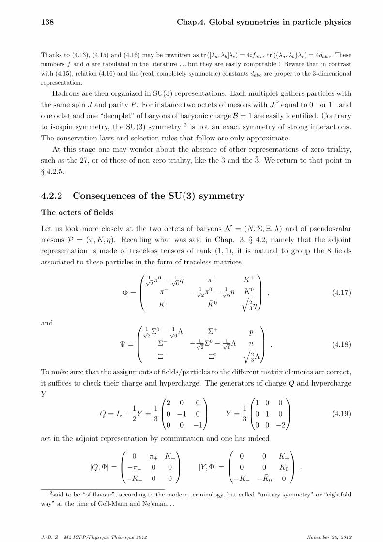
associated to these particles in the form of traceless matrices

� =

0

B

B

@

1p2⇡0 � 1p

6⌘ ⇡+ K+

⇡� � 1p2⇡0 � 1p

6⌘ K0

K� K0q

23⌘

1

C

C

A

, (4.17)

and

=

0

B

B

@

1p2⌃0 � 1p

6⇤ ⌃+ p

⌃� � 1p2⌃0 � 1p

6⇤ n

⌅� ⌅0q

23⇤

1

C

C

A

. (4.18)

To make sure that the assignments of fields/particles to the di↵erent matrix elements are correct,

it su�ces to check their charge and hypercharge. The generators of charge Q and hypercharge

Y

Q = Iz +1

2Y =

1

3

0

B

@

2 0 0

0 �1 0

0 0 �1

1

C

A

Y =1

3

0

B

@

1 0 0

0 1 0

0 0 �2

1

C

A

(4.19)

act in the adjoint representation by commutation and one has indeed

[Q,�] =

0

B

@

0 ⇡+ K+

�⇡� 0 0

�K� 0 0

1

C

A

[Y,�] =

0

B

@

0 0 K+

0 0 K0

�K� �K0 0

1

C

A

.

2said to be “of flavour”, according to the modern terminology, but called “unitary symmetry” or “eightfoldway” at the time of Gell-Mann and Ne’eman. . .



Exercises : (i) with no further calculation, what is [Iz,�] ? Check.

(ii) Compute tr�2, and explain why the result justifies the choice of normalization of the matrix

elements in (4.17). See also Problem 2.c.

Tensor products in SU(3) and invariant couplings

Recall that in SU(3), with notations of Chap. 3,

8⌦ 8 = 1� 8� 8� 10� 10� 27 . (4.20)

Let us show that this has immediate implications on the number of invariant couplings between

fields.

• We want to write an SU(3) invariant Lagrangian involving the previous octets of fields

� and . What is the number of independent “Yukawa couplings”, i.e. of the form � ,

that are invariant under SU(3)? In other words, what is the number of (linearly independent)

invariants in 8⌦ 8⌦ 8 ? According to a reasoning already done in Chap 2. § 3.2, this number

equals the number of times the representation 8 appears in 8 ⌦ 8, hence, according to (4.20),

2. There are thus two independent invariant Yukawa couplings. If the two octets and � are

written as traceless 3⇥ 3 matrices as in (4.17) and (4.18), = { ij } and � = {� i

k }, these two

couplings read

tr � = ij

ki �

jk and tr � = i

j �k

i j

k (4.21)

(this compact writing omits indices of Dirac spinors, a possible �5 matrix, etc). An often

preferred expression uses the sum and di↵erence of these two terms, hence tr [�, ] and

tr {�, }, traditionally called f term and d term, by reference to (4.15) and (4.16).

• Another question of the same nature is: what is a priori the number of SU(3) invariant

amplitudes in the scattering of two particles belonging to the octets N and P : Ni + Pi !Nf + Pf ? (One takes only SU(3) invariance into account and does not consider possible

discrete symmetries.) The issue is thus the number of invariants in the fourth tensor power

of representation 8. Or equivalently, the number of times the same representation appears in

the two products 8 ⌦ 8 and 8 ⌦ 8. If mi are the multiplicities appearing in 8 ⌦ 8, namely

m1 = 1, m8 = 2, etc, see (4.20), this number isP

i m2i = 8. There are thus eight invariant

amplitudes. In other words, one may write a priori the scattering amplitude in the form

hNfPf |T |NiPi i = (4.22)8

X

r=1

Ar(s, t) h (I, Iz, Y )(Nf

), (I, Iz, Y )(Pf

)|r, (I, Iz, Y )(r) ih r, (I, Iz, Y )(r)|(I, Iz, Y )(Ni

), (I, Iz, Y )(Pi

) i

(with s and t the usual relativistic invariants s = (p1 + p2)2, t = (p1 � p3)2), and all the

dependence in the nature of the scattered particles, identified by the values of their isospin and

hypercharge, is contained in SU(3) Clebsch-Gordan coe�cients.• Let �i, i = 1, 2, 3, 4 be four distinct octet fields. How many quartic (degree 4) SU(3) invariant couplings

may be formed with these four fields? On the one hand, the previous argument gives 8 couplings; on theother hand, it is clear that terms tr (�P1

�P2

�P3

�P4

) and tr (�P1

�P2

) tr (�P3

�P4

) are invariant under allpermutations P . A quick counting leads to 9 di↵erent terms, in contradiction with the previous argument.Where is the catch ? For more, go to the Problem 1 at the end of this chapter. . .



4.2.3 Electromagnetic breaking of the SU(3) symmetry

The SU(3) symmetry is broken, as we said, by strong interactions. Of course, just like the

isospin SU(2) symmetry, it is also broken by electromagnetic and by weak interactions. We

won’t examine the latter but describe now two consequences of the strong and electromagnetic

breakings.

The interaction Lagrangian of a particle of charge q with the electromagnetic field A reads

Lem = �qjµAµ (4.23)

where j is the electric current. The field A is invariant under SU(3) transformations, but how

does j transform? One knows the transformation of its charge Q =R

d3xj0(x, t), since following

(4.12), Q is a linear combination of two generators Y and Iz. Q thus transforms according to

the adjoint representation (8, alias (1, 1) in terms of Dynkin labels). And it is natural to assume

that the current j also transforms in the same way. This is indeed what is found when the

current jµ is regarded as the Noether current of the U(1) symmetry (exercise, check it).

Magnetic moments

The electromagnetic form factors of the baryon octet are defined as

hB|jµ(x)|B0 i = eikxu(FBB0

e (k2)�µ + FBB0

m (k2)�µ⌫k⌫)u0 (4.24)

where u and u0 are Dirac spinors which describe respectively the baryons B and B0 ; k is the

four-momentum transfer from B0 to B. Fe is the electric form factor, if B = B0, Fe(0) =

qB, the electric charge of B, whereas Fm is the magnetic form factor and FBBm (0) gives the

magnetic moment of baryon B. One wants to compute these form factors to first order in the

electromagnetic coupling and to zeroth order in the other terms that might break the SU(3)

symmetry.

From a group theoretical point of view, the matrix element hB|jµ(x)|B0 i comes under the

Wigner-Eckart theorem: there are two ways to project 8 ⇥ 8 on 8 (see (4.20)), (or also, there

are two ways to construct an invariant with 8 ⌦ 8 ⌦ 8). There are thus two “reduced matrix

elements”, hence two independent amplitudes for each of the two form factors, dressed with

SU(3) Clebsch-Gordan coe�cients. By an argument similar to (4.21), one finds that one may

write

FBB0

e,m (k2) = F (1)e,m(k2) tr BQB0 + F (2)

e,m(k2) tr BB0Q

where Q is the matrix of (4.19)

Q =

0

B

@

23

0 0

0 �13

0

0 0 �13

1

C

A

,

and tr BQB0 means the coe�cient of BB0 in the matrix trace tr Q , and likewise for tr BB0Q.

For example, the magnetic moment of the neutron µ(n) is proportional to the magnetic term in



nn, namely �13(F (1)

m + F (2)m ). The four functions F (1,2)

e,m are unknown (their computation would

involve the theory of strong interactions) but one may eliminate them and find relations

µ(n) = µ(⌅0) = 2µ(⇤) = �2µ(⌃0) µ(⌃+) = µ(p) (4.25)

µ(⌅�) = µ(⌃�) = �(µ(p) + µ(n)) µ(⌃0 ! ⇤) =

p3

2µ(n) ,

where the last quantity is the transition magnetic moment ⌃0 ! ⇤. These relations are in

qualitative agreement with experimental data.The magnetic moments of “hyperons” (baryons of higher mass than the nucleons) are measured by their spin

precession in a magnetic field or in transitions within “exotic atoms” (i.e. in the nucleus of which a nucleon hasbeen substituted for a hyperon). The transition magnetic moment ⌃0 ! ⇤ is determined from the cross-section⇤ ! ⌃0 in the Coulomb field of a heavy nucleus. One reads in tables

µ(p) = 2.792847351± 0.000000028 µN µ(n) = �1.9130427± 0.0000005 µN

µ(⇤) = �0.613± 0.004 µN |µ(⌃0 ! ⇤)| = 1.61± 0.08 µN (4.26)

µ(⌃+) = 2.458± 0.010 µN µ(⌃�) = �1.160± 0.025 µN

µ(⌅0) = �1.250± 0.014 µN µ(⌅�) = �0.6507± 0.0025 µN

where µN is the nuclear magneton, µN = e~2mp

= 3.152 10�14 MeV T�1.

Electromagnetic mass splittings

With similar assumptions and methods, one may also find relations between mass splittings of particles withsame hypercharge and isospin I but di↵erent charge, due to electromagnetic interactions, see Problem 3.

4.2.4 “Strong” mass splittings. Gell-Mann–Okubo mass formula

In view of the discrepancies between masses within a SU(3) multiplet, the mass term in the

Lagrangian (or Hamiltonian) cannot be an invariant of SU(3). Gell-Mann and Okubo made

the assumption that the non invariant term �M transforms under the representation 8, more

precisely, since it must have vanishing isospin and hypercharge, that it transforms like the ⌘

or ⇤ component of octets. One is thus led to consider matrix elements hH|�M |H i for the

hadrons H of a multiplet, and to appeal once more to Wigner–Eckart theorem. According to

the decomposition rules of tensor products given in Chap. 3, the representation 8 appears at

most twice in the product of an irreducible representation of SU(3) by its conjugate, (check it,

recalling that 8 = 3 ⌦ 3 1) ; there are at most two independent amplitudes describing mass

splittings within the multiplet, which leads to relations between these mass splittings.An elegant argument enables one to avoid the computation of Clebsch–Gordan coe�cients and to find these

two amplitudes in any representation. As the eight infinitesimal generators transform themselves according tothe representation 8 (adjoint representation), they may be set as before into a 3⇥ 3 matrix

G =

0

B

@

1

2

Y + Iz

p2I

+

⇤p2I�

1

2

Y � Iz ⇤⇤ ⇤ �Y

1

C

A

where the ⇤ stand for strangeness-changing generators that are of no concern to us here. (Note that G11

=Iz + 1

2

Y = Q, the electric charge, is invariant under the action (by commutation with G) of generators X =



0

B

@

0 0 00 ⇤ ⇤0 ⇤ ⇤

1

C

A

which preserve the electric charge.) One seeks two combinations of the generators Iz and Y

transforming like the element (3, 3) of that matrix. One is of course Y itself, the other is given by the element(3, 3) of the cofactor of G, cofG

33

= 1

4

Y 2 � I2

z � 2I+

I� = 1

4

Y 2 � ~I2.

One gets in that way a mass formula for any representation (any multiplet)

M = m1 + m2Y + m3(I(I + 1)� 1

4Y 2) (4.27)

which leaves three undetermined constants (that depend on the multiplet). For example for

the baryon octet, one has four experimental masses, which leads to a sum rule

M⌅ + MN

2=

3M⇤ + M⌃

4(4.28)

which is experimentally well verified: one finds 1128,5 MeV/c2 in the left hand side, 1136

MeV/c2 in the rhs3. For the decuplet, show that the same formula gives equal mass di↵erences

between the four particles �, ⌃⇤, ⌅⇤ and ⌦�. The latter result led to an accurate prediction of

the existence and mass of the ⌦� particle, which was regarded as one of the major achievments

of SU(3). For the octet of pseudoscalar mesons, the mass formula is empirically better verified

in terms of the square masses

m2K =

3m2⌘ + m2

⇡

4.

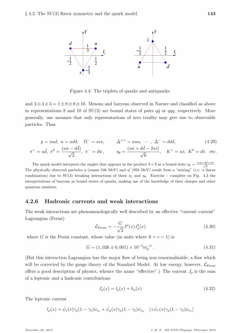
4.2.5 Quarks

The representations 3 and 3 are so far absent from the scene: among the observed particles,

no “triplet” seems to show up. The Gell-Mann–Zweig model makes the assumption that a

triplet (representation 3) of quarks (u, d, s) (“up”, “down” and “strange”) and its conjugate

representation 3 of antiquarks (u, d, s) encompass the elementary constituents of all hadrons

(known at the time). Their charges and hypercharges are respectively

Quarks u d s u d s

Isospin Iz12�1

20 �1

212

0

Baryonic charge B 13

13

13�1

3�1

3�1

3

Strangeness S 0 0 �1 0 0 1

Hypercharge Y 13

13�2

3�1

3�1

323

Electric charge Q 23�1

3�1

3�2

313

13

Table 1. Quantum numbers of quarks u, d, s

One recalls (Chap. 3 §4) that any irreducible representation of SU(3) appears in the de-

composition of iterated tensor products of representations 3 and 3 ; in particular, 3⌦ 3 = 1� 8

3The observed masses of these hadrons are MN ⇡ 939 MeV/c2, M⇤

= 1116 MeV/c2, M⌃

⇡ 1195 MeV/c2,M

⌅

⇡ 1318 MeV/c2 ; those of pseudoscalar mesons m⇡ ⇡ 137 MeV/c2, mK ⇡ 496 MeV/c2 and m⌘ =548 MeV/c2. For the decuplet, M

�

⇡ 1232 MeV/c2, M⌃

⇤ ⇡ 1385 MeV/c2, M⌅

⇤ ⇡ 1530 MeV/c2, M⌦

⇡1672 MeV/c2.



Iz

1

2

1

2!

!1

2

!2

3

Iz

Y Y

1

2

d u

s

1

3

du

s

Figure 4.4: The triplets of quarks and antiquarks.

and 3⌦ 3⌦ 3 = 1� 8� 8� 10. Mesons and baryons observed in Nature and classified as above

in representations 8 and 10 of SU(3) are bound states of pairs qq or qqq, respectively. More

generally, one assumes that only representations of zero triality may give rise to observable

particles. Thus

p = uud, n = udd, ⌦� = sss, �++ = uuu, · · · , �� = ddd, (4.29)

⇡+ = ud, ⇡0 =(uu� dd)p

2, ⇡� = du , ⌘8 =

(uu + dd� 2ss)p6

, K+ = us, K0 = ds etc.

The quark model interprets the singlet that appears in the product 3⇥ 3 as a bound state ⌘1

= (uu+d ¯d+ss)p3

.The physically observed particles ⌘ (masse 548 MeV) and ⌘0 (958 MeV) result from a “mixing” (i.e. a linearcombination) due to SU(3) breaking interactions of these ⌘

1

and ⌘8

. Exercise : complete on Fig. 4.3 theinterpretations of baryons as bound states of quarks, making use of the knowledge of their charges and otherquantum numbers.

4.2.6 Hadronic currents and weak interactions

The weak interactions are phenomenologically well described by an e↵ective “current–current”

Lagrangian (Fermi)

LFermi = � Gp2J⇢(x)J†

⇢(x) (4.30)

where G is the Fermi constant, whose value (in units where ~ = c = 1) is

G = (1, 026± 0, 001)⇥ 10�5m�2p . (4.31)

(But this interaction Lagrangian has the major flaw of being non renormalisable, a flaw which

will be corrected by the gauge theory of the Standard Model. At low energy, however, LFermi

o↵ers a good description of physics, whence the name “e↵ective”.) The current J⇢ is the sum

of a leptonic and a hadronic contributions

J⇢(x) = l⇢(x) + h⇢(x) (4.32)

The leptonic current

l⇢(x) = e(x)�⇢(1� �5) ⌫e

+ µ(x)�⇢(1� �5) ⌫µ

[+ ⌧ (x)�⇢(1� �5) ⌫⌧

]



is the sum of contributions of the lepton families (or generations), e, µ (and ⌧ that we omit in

this first approach). The hadronic current, if one restricts to the first two generations, reads

h⇢ = cos ✓C h(�S=0)⇢ + sin ✓C h(�S=1)

⇢ (4.33)

i.e. a combination of strangeness-conserving and non-conserving currents, weighted by the

Cabibbo angle ✓C ⇡ 0, 25. (This “mixing” extends to the introduction of the third generation,

see next Chapter.) Finally each of these currents h(�S=0)⇢ , h(�S=1)

⇢ has the “V � A” form,

following an idea of Feynman and Gell-Mann, i.e. is a combination of vector and axial currents,

h(�S=0)⇢ = (V 1

⇢ � iV 2⇢ )� (A1

⇢ � iA2⇢) (4.34)

h(�S=1)⇢ = (V 4

⇢ � iV 5⇢ )� (A4

⇢ � iA5⇢) . (4.35)

The vector currents V 1,2,3⇢ are the Noether currents of isospin, the other components of V⇢ are

those of the SU(3) symmetry. One shows that their conservation (exact for isospin, approximate

for the others) implies that in the matrix element Gh p|h(�S=0)⇢ |n i = up�⇢(GV (q2)�GA(q2)�5)un

measured in beta decay at quasi-vanishing momentum transfer, the vector form factor GV (0) =

G. On the contrary, the axial currents are non conserved and GA(0) is “renormalized” (that is,

dressed) by strong interactions, GA/GV ⇡ 1.22. The electromagnetic current is nothing other

that the combination j⇢ = V 3⇢ + 1p

3V 8⇢ . In the quark model, these hadronic currents have the

form

V a⇢ (x) = q(x)

�a

2�⇢ q(x) Aa

⇢(x) = q(x)�a

2�⇢�5 q(x) . (4.36)

We will meet them again in the Standard Model.

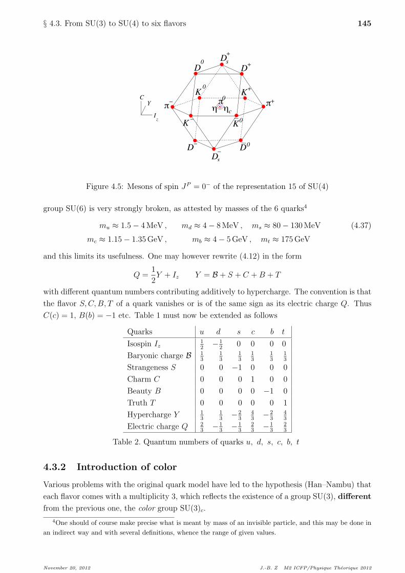
4.3 From SU(3) to SU(4) to six flavors

4.3.1 New flavors

The discovery in the mid 70’s of particles of a new type revived the game: these particles

carry another quantum number, “charm” (whose existence had been postulated beforehand

by Glashow, Iliopoulos and Maiani and by Kobayashi and Maskawa for two di↵erent reasons).

This introduces a third direction in the space of internal symmetries, on top of isospin and

strangeness (or hypercharge). The relevant group is SU(4), which is more severely broken than

SU(3). Particles fall into representations of that SU(4), etc. A fourth flavor, charm, is thus

added, and a fourth charmed quark c constitutes with u, d, s the representation 4 of SU(4), as

inobservable as the 3 of SU(3), according to the same principle.

As for today, one believes there are in total six flavors, the last two being beauty or bottomness

and truth (or topness ??), hence two additional quarks b and t. B mesons, which are bound

states ub, db etc, are observed in everyday experiments, in particular at LHCb, whereas the

experimental evidence for the existence of the t quark is more indirect. The hypothetical flavor


§ 4.3. From SU(3) to SU(4) to six flavors 145

!" +

D+

+D

0

D

c

0

0

K K+

K0!

K

"!

!D D

0

Ds

s

!Y

I

C

z

!

"

Figure 4.5: Mesons of spin JP = 0� of the representation 15 of SU(4)

group SU(6) is very strongly broken, as attested by masses of the 6 quarks4

mu ⇡ 1.5� 4 MeV , md ⇡ 4� 8 MeV , ms ⇡ 80� 130 MeV (4.37)

mc ⇡ 1.15� 1.35 GeV , mb ⇡ 4� 5 GeV , mt ⇡ 175 GeV

and this limits its usefulness. One may however rewrite (4.12) in the form

Q =1

2Y + Iz Y = B + S + C + B + T

with di↵erent quantum numbers contributing additively to hypercharge. The convention is that

the flavor S,C, B, T of a quark vanishes or is of the same sign as its electric charge Q. Thus

C(c) = 1, B(b) = �1 etc. Table 1 must now be extended as follows

Quarks u d s c b t

Isospin Iz12�1

20 0 0 0

Baryonic charge B 13

13

13

13

13

13

Strangeness S 0 0 �1 0 0 0

Charm C 0 0 0 1 0 0

Beauty B 0 0 0 0 �1 0

Truth T 0 0 0 0 0 1

Hypercharge Y 13

13�2

343�2

343

Electric charge Q 23�1

3�1

323�1

323

Table 2. Quantum numbers of quarks u, d, s, c, b, t

4.3.2 Introduction of color

Various problems with the original quark model have led to the hypothesis (Han–Nambu) that

each flavor comes with a multiplicity 3, which reflects the existence of a group SU(3), di↵erent

from the previous one, the color group SU(3)c.

4One should of course make precise what is meant by mass of an invisible particle, and this may be done inan indirect way and with several definitions, whence the range of given values.



Considerations leading to that triplicating hypothesis are first the study of the �++ particle, with spin 3/2,made of 3 quarks u. This system of 3 quarks has a spin 3/2 and an orbital angular momentum L = 0, whichgive it a symmetric wave function, in contradiction with the fermionic character of quarks. The additionalcolor degree of freedom allows an extra antisymmetrization, (which leads to a singlet state of color), and thusremoves the problem. On the other hand, the decay amplitude of ⇡0 ! 2� is proportional to the sum

P

Q2Iz

over the set of fermionic constituents of the ⇡0. The proton, with its charge Q = 1 and Iz = 1

2

, gives a valuein agreement with experiment. Quarks (u, d, s) with Q = ( 2

3

, 1

3

,� 1

3

) and Iz = ( 1

2

,� 1

2

, 0) lead to a result threetimes too small, and color multiplicity corrects it to the right value.

According to the confinement hypothesis, only states of the representation 1 of SU(3)c are

observable. The other states, which are said to be “colored”, are bound in a permanent way

inside hadrons. This applies to quarks, but also to gluons, which are vector particles (spin 1)

transforming by the representation 8 of SU(3)c, whose existence is required by the construction

of the gauge theory of strong interactions, Quantum Chromodynamics (QCD), see Chap. 5.

To be more precise, the confinement hypothesis applies to zero or low temperature, and quark or gluondeconfinement may occur in hadronic matter at high temperature or high density (within the “quark gluonplasma”).

The quark model with its color group SU(3)c is now regarded as part of quantum chromo-

dynamics. The six flavors of quarks are grouped into three “generations”, (u, d), (c, s), (t, b),

which are in correspondence with three generations of leptons, (e�, ⌫e), (µ�, ⌫µ), (⌧�, ⌫⌧ ). That

correspondence is important for the consistency of the Standard Model (anomaly cancellation),

see next chapter.

?

Further references for Chapter 4

On flavor SU(3), the standard reference containing all historical papers is

M. Gell-Mann and Y. Ne’eman, The Eightfold Way, Benjamin 1964.

In particular one finds there tables of SU(3) Clebsch-Gordan coe�cients by J.J. de Swart.

In the discussion of SU(3) breakings, I followed

S. Coleman, Aspects of Symmetry, Cambridge Univ. Press 1985.

For a more recent presentation of flavor physics, see

K. Huang, Quarks, Leptons and Gauge Fields, World Scientific 1992.

All the properties of particles mentionned in this chapter may be found in the tables of the

Particle Data Group, on line on the site http://pdg.lbl.gov/2012/reviews/contents sports.html

?


§ 4.3. From SU(3) to SU(4) to six flavors 147

Exercises for chapter 4

A. Sigma model and chiral symmetry breaking

Consider the Lagrangian (4.10) and define W = � + i⇡⇡⇡⌧⌧⌧ .

1. Compute det W . Show that one may write L in terms of L,R and W as

L = Ri/@ R + Li/@ L + g( LW R + RW † L) + LK � 1

2m2 det W � �

4(det W )2

where LK is the kinetic term of the fields (�,⇡⇡⇡). One may also give that term the form LK =12(det @0W �P3

i=1 det @iW ) (which looks a bit odd, but which is indeed Lorentz invariant!).

2. Show that L is invariant under transformations of SU(2) ⇥ SU(2) with L ! U L,

R ! V R, provided W transforms in a way to be specified. Justify the assertion made in

§4.1.2 : L, R and W transform respectively under the representations (12, 0), (0, 1

2) and (1

2, 1

2).

3. If the field W acquires a vev v, for example along the direction of �, h� i = v, show that

the field acquires a mass M = �gv.

B. Changes of basis in SU(3)

In SU(3), write the change of basis which transforms the weights ⇤1, ⇤2 of Chap. 3 into the

axes used in figures 2, 3 and 4. Derive the transformation of the coordinates (�1,�2) (Dynkin

labels) into the physical coordinates (Iz, Y ). What is the dimension of the representation of

SU(3) expressed in terms of the isospin and hypercharge of its highest weight?

C. Gell-Mann–Okubo formula

Complete and justify all the arguments sketched in § 4.2.2, 4.2.3 and 4.2.4. In particular check

that the formula (4.27) does lead for the baryon octet to the rule (4.28), and for the decuplet,

to constant mass splittings.

D. Counting amplitudes

How many independent amplitudes are necessary to describe the scattering BD ! BD, where

B and D refer to the baryonic octet and decuplet ?

Problems

1. SU(3) invariant four-field couplings

Consider a Hermitian, 3⇥ 3 and traceless matrix A.

a. Show that its characteristic equation

A3 � (tr A)A2 +1

2

�

(tr A)2 � tr A2�

A� det A = 0

implies a relation between tr A4 and (tr A2)2.

b. If the group SU(3) acts on A by A ! UAU †, show that any sum of products of traces

of powers of A is invariant. We call such a sum an “invariant polynomial in A”. How many

linearly independent such invariant polynomials in A of degree 4 are there?



c. One then “polarises” the identity found in a., which means one writes A =P4

i=1 xiAi

with 4 matrices Ai of the previous type and 4 arbitrary coe�cients xi, and one identifies the

coe�cient of x1x2x3x4. Show that this gives an identity of the form (Burgoyne’s identity)

X

P

tr (AP1AP2AP3AP4) = aX

P

tr (AP1AP2) tr (AP3AP4) (4.38)

with sums over permutations P of 4 elements and a coe�cient a to be determined. How many

distinct terms appear in each side of that identity?

d. How many polynomials of degree 4, quadrilinear in A1, · · · , A4, invariant under the action

of SU(3) Ai ! UAiU † and linearly independent, can one write ? Why is the identity (4.38)

useful ?

2. Hidden invariance of a bosonic Lagrangian

One wants to write a Lagrangian for the field � of the pseudoscalar meson octet, see (4.17).

a. Why is it natural to impose that this Lagrangian be even in the field � ?

b. Using the results of Problem 1., write the most general form of an SU(3) invariant

Lagrangian, of degree less or equal to 4 (for renormalizability) and even in �.

c. One then writes each complex field by making explicit its real and imaginary parts, for

example K+ = 1p2(K1 � iK2), K� = 1p

2(K1 + iK2), and likewise with K0, K0 and with ⇡±.

Compute tr �2 with that parametrization and show that one gets a simple quadratic form in

the 8 real components. What is the invariance group G of that quadratic form? Is G a subgroup

of SU(3)?

d. Conclude that any Lagrangian of degree 4 in � which is invariant under SU(3) is in fact

invariant by this group G.

3. Electromagnetic mass splittings in an SU(3) octet

Preliminary question.

Given a vector space E of dimension d, we denote E ⌦ E the space of rank 2 tensors and

(E ⌦ E)S, resp. (E ⌦ E)A, the spaces of symmetric, resp. antisymmetric, rank 2 tensors, also

called (anti-)symmetrized tensor product. What is the dimension of spaces E ⌦ E, (E ⌦ E)S,

(E ⌦ E)A ?

One assumes that SU(3) is an exact symmetry of strong interactions, and one wants to study

mass splittings due to electromagnetic e↵ects.

a. How many independent mass di↵erences between baryons with the same quantum num-

bers I and Y but di↵erent charges Q (or Iz component), are there in the baryon octet JP = 12

+?

We admit that these electromagnetic e↵ects result from second order perturbations in the

Lagrangian Lem(x) = �qjµ(x)Aµ(x). If |B i is a baryon state, one should thus compute

�MB = hB|(Z

d4xLem)2|B i . (4.39)

For lack of a good way of computing that matrix element, one wants to determine the number

of independent amplitudes that contribute.


Chapter 4 Global symmetries in particle physics - UPMCzuber/Cours/chap4_12e.pdfGlobal symmetries in...

Documents

Transcript of Chapter 4 Global symmetries in particle physics - UPMCzuber/Cours/chap4_12e.pdfGlobal symmetries in...