Chapter 4: Exponential and Logarithmic Functions 4.pdf · Write an exponential function for...

This chapter is part of Precalculus: An Investigation of Functions © Lippman & Rasmussen 2017. This material is licensed under a Creative Commons CC-BY-SA license.

Chapter 4: Exponential and Logarithmic Functions

Section 4.1 Exponential Functions ............................................................................. 249 Section 4.2 Graphs of Exponential Functions............................................................. 267 Section 4.3 Logarithmic Functions ............................................................................. 277 Section 4.4 Logarithmic Properties............................................................................. 289 Section 4.5 Graphs of Logarithmic Functions ............................................................ 300 Section 4.6 Exponential and Logarithmic Models ...................................................... 308 Section 4.7 Fitting Exponentials to Data .................................................................... 328

Section 4.1 Exponential Functions India is the second most populous country in the world, with a population in 2008 of about 1.14 billion people. The population is growing by about 1.34% each year1. We might ask if we can find a formula to model the population, P, as a function of time, t, in years after 2008, if the population continues to grow at this rate. In linear growth, we had a constant rate of change – a constant number that the output increased for each increase in input. For example, in the equation 43)( += xxf , the slope tells us the output increases by three each time the input increases by one. This population scenario is different – we have a percent rate of change rather than a constant number of people as our rate of change. To see the significance of this difference consider these two companies: Company A has 100 stores, and expands by opening 50 new stores a year Company B has 100 stores, and expands by increasing the number of stores by 50% of their total each year. Looking at a few years of growth for these companies: 1 World Bank, World Development Indicators, as reported on http://www.google.com/publicdata, retrieved August 20, 2010

http://www.google.com/publicdata

Chapter 4 250

Year Stores, company A Stores, company B 0 100 Starting with 100 each

100

1 100 + 50 = 150 They both grow by 50 stores in the first year.

100 + 50% of 100 100 + 0.50(100) = 150

2 150 + 50 = 200 Store A grows by 50, Store B grows by 75

150 + 50% of 150 150 + 0.50(150) = 225

3 200 + 50 = 250 Store A grows by 50, Store B grows by 112.5

225 + 50% of 225 225 + 0.50(225) = 337.5

Notice that with the percent growth, each year the company is grows by 50% of the current year’s total, so as the company grows larger, the number of stores added in a year grows as well. To try to simplify the calculations, notice that after 1 year the number of stores for company B was:

)100(50.0100 + or equivalently by factoring 150)50.01(100 =+

We can think of this as “the new number of stores is the original 100% plus another 50%”. After 2 years, the number of stores was:

)150(50.0150 + or equivalently by factoring )50.01(150 + now recall the 150 came from 100(1+0.50). Substituting that,

225)50.01(100)50.01)(50.01(100 2 =+=++ After 3 years, the number of stores was:

)225(50.0225 + or equivalently by factoring )50.01(225 + now recall the 225 came from 2)50.01(100 + . Substituting that,

5.337)50.01(100)50.01()50.01(100 32 =+=++ From this, we can generalize, noticing that to show a 50% increase, each year we multiply by a factor of (1+0.50), so after n years, our equation would be

nnB )50.01(100)( += In this equation, the 100 represented the initial quantity, and the 0.50 was the percent growth rate. Generalizing further, we arrive at the general form of exponential functions.

Section 4.1 Exponential Functions 251

Exponential Function An exponential growth or decay function is a function that grows or shrinks at a constant percent growth rate. The equation can be written in the form

xraxf )1()( += or xabxf =)( where b = 1+r Where a is the initial or starting value of the function r is the percent growth or decay rate, written as a decimal b is the growth factor or growth multiplier. Since powers of negative numbers behave strangely, we limit b to positive values.

To see more clearly the difference between exponential and linear growth, compare the two tables and graphs below, which illustrate the growth of company A and B described above over a longer time frame if the growth patterns were to continue.

years Company A Company B 2 200 225 4 300 506 6 400 1139 8 500 2563

10 600 5767 Example 1

Write an exponential function for India’s population, and use it to predict the population in 2020. At the beginning of the chapter we were given India’s population of 1.14 billion in the year 2008 and a percent growth rate of 1.34%. Using 2008 as our starting time (t = 0), our initial population will be 1.14 billion. Since the percent growth rate was 1.34%, our value for r is 0.0134. Using the basic formula for exponential growth xraxf )1()( += we can write the formula, ttf )0134.01(14.1)( += To estimate the population in 2020, we evaluate the function at t = 12, since 2020 is 12 years after 2008.

337.1)0134.01(14.1)12( 12 ≈+=f billion people in 2020

Chapter 4 252

Try it Now 1. Given the three statements below, identify which represent exponential functions. A. The cost of living allowance for state employees increases salaries by 3.1% each year. B. State employees can expect a $300 raise each year they work for the state. C. Tuition costs have increased by 2.8% each year for the last 3 years. Example 2

A certificate of deposit (CD) is a type of savings account offered by banks, typically offering a higher interest rate in return for a fixed length of time you will leave your money invested. If a bank offers a 24 month CD with an annual interest rate of 1.2% compounded monthly, how much will a $1000 investment grow to over those 24 months? First, we must notice that the interest rate is an annual rate, but is compounded monthly, meaning interest is calculated and added to the account monthly. To find the monthly interest rate, we divide the annual rate of 1.2% by 12 since there are 12 months in a year: 1.2%/12 = 0.1%. Each month we will earn 0.1% interest. From this, we can set up an exponential function, with our initial amount of $1000 and a growth rate of r = 0.001, and our input m measured in months.

m

mf

+=

12012.11000)(

mmf )001.01(1000)( += After 24 months, the account will have grown to 24(24) 1000(1 0.001) $1024.28f = + =

Try it Now 2. Looking at these two equations that represent the balance in two different savings

accounts, which account is growing faster, and which account will have a higher balance after 3 years?

( )ttA 05.11000)( = ( )ttB 075.1900)( =

In all the preceding examples, we saw exponential growth. Exponential functions can also be used to model quantities that are decreasing at a constant percent rate. An example of this is radioactive decay, a process in which radioactive isotopes of certain atoms transform to an atom of a different type, causing a percentage decrease of the original material over time.


Example 3 Bismuth-210 is an isotope that radioactively decays by about 13% each day, meaning 13% of the remaining Bismuth-210 transforms into another atom (polonium-210 in this case) each day. If you begin with 100 mg of Bismuth-210, how much remains after one week? With radioactive decay, instead of the quantity increasing at a percent rate, the quantity is decreasing at a percent rate. Our initial quantity is a = 100 mg, and our growth rate will be negative 13%, since we are decreasing: r = -0.13. This gives the equation:

dddQ )87.0(100)13.01(100)( =−= This can also be explained by recognizing that if 13% decays, then 87 % remains. After one week, 7 days, the quantity remaining would be

73.37)87.0(100)7( 7 ==Q mg of Bismuth-210 remains. Try it Now 3. A population of 1000 is decreasing 3% each year. Find the population in 30 years. Example 4

T(q) represents the total number of Android smart phone contracts, in thousands, held by a certain Verizon store region measured quarterly since January 1, 2016, Interpret all the parts of the equation 3056.231)64.1(86)2( 2 ==T . Interpreting this from the basic exponential form, we know that 86 is our initial value. This means that on Jan. 1, 2016 this region had 86,000 Android smart phone contracts. Since b = 1 + r = 1.64, we know that every quarter the number of smart phone contracts grows by 64%. T(2) = 231.3056 means that in the 2nd quarter (or at the end of the second quarter) there were approximately 231,306 Android smart phone contracts.

Finding Equations of Exponential Functions In the previous examples, we were able to write equations for exponential functions since we knew the initial quantity and the growth rate. If we do not know the growth rate, but instead know only some input and output pairs of values, we can still construct an exponential function. Example 5

In 2009, 80 deer were reintroduced into a wildlife refuge area from which the population had previously been hunted to elimination. By 2015, the population had grown to 180 deer. If this population grows exponentially, find a formula for the function.

Chapter 4 254

By defining our input variable to be t, years after 2009, the information listed can be written as two input-output pairs: (0,80) and (6,180). Notice that by choosing our input variable to be measured as years after the first year value provided, we have effectively “given” ourselves the initial value for the function: a = 80. This gives us an equation of the form

tbtf 80)( = . Substituting in our second input-output pair allows us to solve for b:

6180 80b= Divide by 80 6 180 9

80 4b = = Take the 6th root of both sides.

69 1.14474

b = =

This gives us our equation for the population:

ttf )1447.1(80)( = Recall that since b = 1+r, we can interpret this to mean that the population growth rate is r = 0.1447, and so the population is growing by about 14.47% each year.

In this example, you could also have used (9/4)^(1/6) to evaluate the 6th root if your calculator doesn’t have an nth root button. In the previous example, we chose to use the xabxf =)( form of the exponential function rather than the xraxf )1()( += form. This choice was entirely arbitrary – either form would be fine to use. When finding equations, the value for b or r will usually have to be rounded to be written easily. To preserve accuracy, it is important to not over-round these values. Typically, you want to be sure to preserve at least 3 significant digits in the growth rate. For example, if your value for b was 1.00317643, you would want to round this no further than to 1.00318. In the previous example, we were able to “give” ourselves the initial value by clever definition of our input variable. Next, we consider a situation where we can’t do this.


Example 6 Find a formula for an exponential function passing through the points (-2,6) and (2,1). Since we don’t have the initial value, we will take a general approach that will work for any function form with unknown parameters: we will substitute in both given input-output pairs in the function form xabxf =)( and solve for the unknown values, a and b. Substituting in (-2, 6) gives 26 −= ab Substituting in (2, 1) gives 21 ab= We now solve these as a system of equations. To do so, we could try a substitution approach, solving one equation for a variable, then substituting that expression into the second equation. Solving 26 −= ab for a:

22

6 6a bb−= =

In the second equation, 21 ab= , we substitute the expression above for a:

6389.061

61

61)6(1

4

4

4

22

≈=

=

=

=

b

b

bbb

Going back to the equation 26ba = lets us find a:

4492.2)6389.0(66 22 === ba Putting this together gives the equation xxf )6389.0(4492.2)( =

Try it Now 4. Given the two points (1, 3) and (2, 4.5) find the equation of an exponential function

that passes through these two points.

Chapter 4 256

Example 7 Find an equation for the exponential function graphed. The initial value for the function is not clear in this graph, so we will instead work using two clearer points. There are three clear points: (-1, 1), (1, 2), and (3, 4). As we saw in the last example, two points are sufficient to find the equation for a standard exponential, so we will use the latter two points. Substituting in (1,2) gives 12 ab= Substituting in (3,4) gives 34 ab=

Solving the first equation for a gives b

a 2= .

Substituting this expression for a into the second equation:

34 ab=

bbb

b

33 224 == Simplify the right-hand side

2

224

2

2

±=

=

=

b

bb

Since we restrict ourselves to positive values of b, we will use 2=b . We can then go back and find a:

22

22===

ba

This gives us a final equation of xxf )2(2)( = .

Compound Interest In the bank certificate of deposit (CD) example earlier in the section, we encountered compound interest. Typically bank accounts and other savings instruments in which earnings are reinvested, such as mutual funds and retirement accounts, utilize compound interest. The term compounding comes from the behavior that interest is earned not on the original value, but on the accumulated value of the account.


In the example from earlier, the interest was compounded monthly, so we took the annual interest rate, usually called the nominal rate or annual percentage rate (APR) and divided by 12, the number of compounds in a year, to find the monthly interest. The exponent was then measured in months. Generalizing this, we can form a general formula for compound interest. If the APR is written in decimal form as r, and there are k compounding periods per year, then the interest per compounding period will be r/k. Likewise, if we are interested in the value after t years, then there will be kt compounding periods in that time.

Compound Interest Formula Compound Interest can be calculated using the formula

kt

kratA

+= 1)(

Where A(t) is the account value t is measured in years a is the starting amount of the account, often called the principal r is the annual percentage rate (APR), also called the nominal rate k is the number of compounding periods in one year

Example 8

If you invest $3,000 in an investment account paying 3% interest compounded quarterly, how much will the account be worth in 10 years? Since we are starting with $3000, a = 3000 Our interest rate is 3%, so r = 0.03 Since we are compounding quarterly, we are compounding 4 times per year, so k = 4 We want to know the value of the account in 10 years, so we are looking for A(10), the value when t = 10.

05.4045$403.013000)10(

)10(4

=

+=A

The account will be worth $4045.05 in 10 years.

Chapter 4 258

Example 9 A 529 plan is a college savings plan in which a relative can invest money to pay for a child’s later college tuition, and the account grows tax free. If Lily wants to set up a 529 account for her new granddaughter, wants the account to grow to $40,000 over 18 years, and she believes the account will earn 6% compounded semi-annually (twice a year), how much will Lily need to invest in the account now? Since the account is earning 6%, r = 0.06 Since interest is compounded twice a year, k = 2 In this problem, we don’t know how much we are starting with, so we will be solving for a, the initial amount needed. We do know we want the end amount to be $40,000, so we will be looking for the value of a so that A(18) = 40,000.

801,13$8983.2000,40

)8983.2(000,40206.01)18(000,40

)18(2

≈=

=

+==

a

a

aA

Lily will need to invest $13,801 to have $40,000 in 18 years.

Try it now 5. Recalculate example 2 from above with quarterly compounding. Because of compounding throughout the year, with compound interest the actual increase in a year is more than the annual percentage rate. If $1,000 were invested at 10%, the table below shows the value after 1 year at different compounding frequencies:

Frequency Value after 1 year Annually $1100 Semiannually $1102.50 Quarterly $1103.81 Monthly $1104.71 Daily $1105.16

If we were to compute the actual percentage increase for the daily compounding, there was an increase of $105.16 from an original amount of $1,000, for a percentage increase

of 10516.01000

16.105= = 10.516% increase. This quantity is called the annual percentage

yield (APY).


Notice that given any starting amount, the amount after 1 year would be k

kraA

+= 1)1( . To find the total change, we would subtract the original amount, then

to find the percentage change we would divide that by the original amount:

111

−

+=

−

+ k

k

kr

a

akra

Annual Percentage Yield The annual percentage yield is the actual percent a quantity increases in one year. It can be calculated as

11 −

+=

k

krAPY

This is equivalent to finding the value of $1 after 1 year, and subtracting the original dollar. Example 10

Bank A offers an account paying 1.2% compounded quarterly. Bank B offers an account paying 1.1% compounded monthly. Which is offering a better rate? We can compare these rates using the annual percentage yield – the actual percent increase in a year.

Bank A: 012054.014012.01

4

=−

+=APY = 1.2054%

Bank B: 011056.0112011.01

12

=−

+=APY = 1.1056%

Bank B’s monthly compounding is not enough to catch up with Bank A’s better APR. Bank A offers a better rate.

A Limit to Compounding As we saw earlier, the amount we earn increases as we increase the compounding frequency. The table, though, shows that the increase from annual to semi-annual compounding is larger than the increase from monthly to daily compounding. This might lead us to believe that although increasing the frequency of compounding will increase our result, there is an upper limit to this process.

Chapter 4 260

To see this, let us examine the value of $1 invested at 100% interest for 1 year.

Frequency Value Annual $2 Quarterly $2.441406 Monthly $2.613035 Daily $2.714567 Hourly $2.718127 Once per minute $2.718279 Once per second $2.718282

These values do indeed appear to be approaching an upper limit. This value ends up being so important that it gets represented by its own letter, much like how π represents a number.

Euler’s Number: e

e is the letter used to represent the value that k

k

+

11 approaches as k gets big.

718282.2≈e Because e is often used as the base of an exponential, most scientific and graphing calculators have a button that can calculate powers of e, usually labeled ex. Some computer software instead defines a function exp(x), where exp(x) = ex. Because e arises when the time between compounds becomes very small, e allows us to define continuous growth and allows us to define a new toolkit function, ( ) xf x e= .

Continuous Growth Formula Continuous Growth can be calculated using the formula

rxaexf =)( where a is the starting amount r is the continuous growth rate

This type of equation is commonly used when describing quantities that change more or less continuously, like chemical reactions, growth of large populations, and radioactive decay.


Example 11 Radon-222 decays at a continuous rate of 17.3% per day. How much will 100mg of Radon-222 decay to in 3 days? Since we are given a continuous decay rate, we use the continuous growth formula. Since the substance is decaying, we know the growth rate will be negative: r = -0.173

512.59100)3( )3(173.0 ≈= −ef mg of Radon-222 will remain. Try it Now 6. Interpret the following: 0.12( ) 20 tS t e= if S(t) represents the growth of a substance in

grams, and time is measured in days. Continuous growth is also often applied to compound interest, allowing us to talk about continuous compounding. Example 12

If $1000 is invested in an account earning 10% compounded continuously, find the value after 1 year. Here, the continuous growth rate is 10%, so r = 0.10. We start with $1000, so a = 1000. To find the value after 1 year,

17.1105$1000)1( )1(10.0 ≈= ef Notice this is a $105.17 increase for the year. As a percent increase, this is

%517.1010517.01000

17.105== increase over the original $1000.

Notice that this value is slightly larger than the amount generated by daily compounding in the table computed earlier. The continuous growth rate is like the nominal growth rate (or APR) – it reflects the growth rate before compounding takes effect. This is different than the annual growth rate used in the formula xraxf )1()( += , which is like the annual percentage yield – it reflects the actual amount the output grows in a year. While the continuous growth rate in the example above was 10%, the actual annual yield was 10.517%. This means we could write two different looking but equivalent formulas for this account’s growth:

0.10( ) 1000 tf t e= using the 10% continuous growth rate ( ) 1000(1.10517)tf t = using the 10.517% actual annual yield rate.

Chapter 4 262

Important Topics of this Section Percent growth Exponential functions Finding formulas Interpreting equations Graphs Exponential Growth & Decay Compound interest Annual Percent Yield Continuous Growth

Try it Now Answers 1. A & C are exponential functions, they grow by a % not a constant number. 2. B(t) is growing faster (r = 0.075 > 0.05), but after 3 years A(t) still has a higher

account balance 3. tttP )97.0(1000)03.01(1000)( =−=

0071.401)97.0(1000)30( 30 ==P

4. 13 ab= , so b

a 3= ,

25.4 ab= , so 235.4 bb

= . b35.4 =

b = 1.5. 25.1

3==a

( )xxf 5.12)( =

5. 24 months = 2 years. )2(4

4012.11000

+ = $1024.25

6. An initial substance weighing 20g is growing at a continuous rate of 12% per day.


Section 4.1 Exercises For each table below, could the table represent a function that is linear, exponential, or neither?

1. x 1 2 3 4 f(x) 70 40 10 -20

2. x 1 2 3 4 g(x) 40 32 26 22

3. x 1 2 3 4 h(x) 70 49 34.3 24.01

4. x 1 2 3 4 k(x) 90 80 70 60

5. x 1 2 3 4 m(x) 80 61 42.9 25.61

6. x 1 2 3 4 n(x) 90 81 72.9 65.61

7. A population numbers 11,000 organisms initially and grows by 8.5% each year.

Write an exponential model for the population.

8. A population is currently 6,000 and has been increasing by 1.2% each day. Write an exponential model for the population.

9. The fox population in a certain region has an annual growth rate of 9 percent per year. It is estimated that the population in the year 2010 was 23,900. Estimate the fox population in the year 2018.

10. The amount of area covered by blackberry bushes in a park has been growing by 12% each year. It is estimated that the area covered in 2009 was 4,500 square feet. Estimate the area that will be covered in 2020.

11. A vehicle purchased for $32,500 depreciates at a constant rate of 5% each year. Determine the approximate value of the vehicle 12 years after purchase.

12. A business purchases $125,000 of office furniture which depreciates at a constant rate of 12% each year. Find the residual value of the furniture 6 years after purchase.

Chapter 4 264

Find a formula for an exponential function passing through the two points. 13. ( )0, 6 , (3, 750) 14. ( )0, 3 , (2, 75)

15. ( )0, 2000 , (2, 20) 16. ( )0, 9000 , (3, 72)

17. ( )31, , 3, 242

−

18. ( )21, , 1,105

−

19. ( ) ( )2,6 , 3,1− 20. ( )3,4 , (3, 2)−

21. ( )3,1 , (5, 4) 22. ( )2,5 , (6, 9)

23. A radioactive substance decays exponentially. A scientist begins with 100 milligrams of a radioactive substance. After 35 hours, 50 mg of the substance remains. How many milligrams will remain after 54 hours?

24. A radioactive substance decays exponentially. A scientist begins with 110 milligrams of a radioactive substance. After 31 hours, 55 mg of the substance remains. How many milligrams will remain after 42 hours?

25. A house was valued at $110,000 in the year 1985. The value appreciated to $145,000 by the year 2005. What was the annual growth rate between 1985 and 2005? Assume that the house value continues to grow by the same percentage. What did the value equal in the year 2010?

26. An investment was valued at $11,000 in the year 1995. The value appreciated to $14,000 by the year 2008. What was the annual growth rate between 1995 and 2008? Assume that the value continues to grow by the same percentage. What did the value equal in the year 2012?

27. A car was valued at $38,000 in the year 2003. The value depreciated to $11,000 by the year 2009. Assume that the car value continues to drop by the same percentage. What was the value in the year 2013?

28. A car was valued at $24,000 in the year 2006. The value depreciated to $20,000 by the year 2009. Assume that the car value continues to drop by the same percentage. What was the value in the year 2014?

29. If $4,000 is invested in a bank account at an interest rate of 7 per cent per year, find the amount in the bank after 9 years if interest is compounded annually, quarterly, monthly, and continuously.


30. If $6,000 is invested in a bank account at an interest rate of 9 per cent per year, find the amount in the bank after 5 years if interest is compounded annually, quarterly, monthly, and continuously.

31. Find the annual percentage yield (APY) for a savings account with annual percentage rate of 3% compounded quarterly.

32. Find the annual percentage yield (APY) for a savings account with annual percentage rate of 5% compounded monthly.

33. A population of bacteria is growing according to the equation 0.21 ( ) 1 600 tP t e= , with t measured in years. Estimate when the population will exceed 7569.

34. A population of bacteria is growing according to the equation 0.17 ( ) 1 200 tP t e= , with t measured in years. Estimate when the population will exceed 3443.

35. In 1968, the U.S. minimum wage was $1.60 per hour. In 1976, the minimum wage was $2.30 per hour. Assume the minimum wage grows according to an exponential model ( )w t , where t represents the time in years after 1960. [UW]

a. Find a formula for ( )w t . b. What does the model predict for the minimum wage in 1960? c. If the minimum wage was $5.15 in 1996, is this above, below or equal to what

the model predicts?

36. In 1989, research scientists published a model for predicting the cumulative number

of AIDS cases (in thousands) reported in the United States: ( )31980155

10ta t − =

,

where t is the year. This paper was considered a “relief”, since there was a fear the correct model would be of exponential type. Pick two data points predicted by the research model ( )a t to construct a new exponential model ( )b t for the number of cumulative AIDS cases. Discuss how the two models differ and explain the use of the word “relief.” [UW]

Chapter 4 266

37. You have a chess board as pictured, with squares numbered 1 through 64. You also have a huge change jar with an unlimited number of dimes. On the first square you place one dime. On the second square you stack 2 dimes. Then you continue, always doubling the number from the previous square. [UW]

a. How many dimes will you have stacked on the 10th square?

b. How many dimes will you have stacked on the nth square?

c. How many dimes will you have stacked on the 64th square?

d. Assuming a dime is 1 mm thick, how high will this last pile be? e. The distance from the earth to the sun is approximately 150 million km.

Relate the height of the last pile of dimes to this distance.

Section 4.2 Graphs of Exponential Functions 267

Section 4.2 Graphs of Exponential Functions Like with linear functions, the graph of an exponential function is determined by the values for the parameters in the function’s formula. To get a sense for the behavior of exponentials, let us begin by looking more closely at the function xxf 2)( = . Listing a table of values for this function:

x -3 -2 -1 0 1 2 3

f(x) 81

41

21 1 2 4 8

Notice that:

1) This function is positive for all values of x. 2) As x increases, the function grows faster and faster (the rate of change

increases). 3) As x decreases, the function values grow smaller, approaching zero. 4) This is an example of exponential growth.

Looking at the function x

xg

=

21)(

x -3 -2 -1 0 1 2 3

g(x) 8 4 2 1 21

41

81

Note this function is also positive for all values of x, but in this case grows as x decreases, and decreases towards zero as x increases. This is an example of exponential decay. You may notice from the table that this function appears to be the horizontal reflection of the

xxf 2)( = table. This is in fact the case:

)(21)2(2)( 1 xgxf

xxx =

===− −−

Looking at the graphs also confirms this relationship. Consider a function of the form xabxf =)( . Since a, which we called the initial value in the last section, is the function value at an input of zero, a will give us the vertical intercept of the graph.

Chapter 4 268

From the graphs above, we can see that an exponential graph will have a horizontal asymptote on one side of the graph, and can either increase or decrease, depending upon the growth factor. This horizontal asymptote will also help us determine the long run behavior and is easy to determine from the graph. The graph will grow when the growth rate is positive, which will make the growth factor b larger than one. When it’s negative, the growth factor will be less than one.

Graphical Features of Exponential Functions

Graphically, in the function xabxf =)( a is the vertical intercept of the graph b determines the rate at which the graph grows. When a is positive, the function will increase if b > 1 the function will decrease if 0 < b < 1 The graph will have a horizontal asymptote at y = 0 The graph will be concave up if a > 0; concave down if a < 0. The domain of the function is all real numbers The range of the function is (0, )∞

When sketching the graph of an exponential function, it can be helpful to remember that the graph will pass through the points (0, a) and (1, ab). The value b will determine the function’s long run behavior: If b > 1, as ∞→x , ∞→)(xf and as −∞→x , 0)( →xf . If 0 < b < 1, as ∞→x , 0)( →xf and as −∞→x , ∞→)(xf . Example 1

Sketch a graph of x

xf

=

314)(

This graph will have a vertical intercept at (0,4), and pass

through the point

34,1 . Since b < 1, the graph will be

decreasing towards zero. Since a > 0, the graph will be concave up. We can also see from the graph the long run behavior: as

∞→x , 0)( →xf and as −∞→x , ∞→)(xf .


To get a better feeling for the effect of a and b on the graph, examine the sets of graphs below. The first set shows various graphs, where a remains the same and we only change the value for b.

Notice that the closer the value of b is to 1, the less steep the graph will be. In the next set of graphs, a is altered and our value for b remains the same.

Notice that changing the value for a changes the vertical intercept. Since a is multiplying the bx term, a acts as a vertical stretch factor, not as a shift. Notice also that the long run behavior for all of these functions is the same because the growth factor did not change and none of these a values introduced a vertical flip.

Chapter 4 270

Example 2 Match each equation with its graph.

x

x

x

x

xkxhxgxf

)7.0(4)()3.1(4)()8.1(2)()3.1(2)(

=

=

=

=

The graph of k(x) is the easiest to identify, since it is the only equation with a growth factor less than one, which will produce a decreasing graph. The graph of h(x) can be identified as the only growing exponential function with a vertical intercept at (0,4). The graphs of f(x) and g(x) both have a vertical intercept at (0,2), but since g(x) has a larger growth factor, we can identify it as the graph increasing faster.

Try it Now 1. Graph the following functions on the same axis:

xxf )2()( = ; xxg )2(2)( = ; xxh )2/1(2)( = .

Transformations of Exponential Graphs While exponential functions can be transformed following the same rules as any function, there are a few interesting features of transformations that can be identified. The first was seen at the beginning of the section – that a horizontal reflection is equivalent to a change in the growth factor. Likewise, since a is itself a stretch factor, a vertical stretch of an exponential corresponds with a change in the initial value of the function.


Next consider the effect of a horizontal shift on an exponential function. Shifting the function xxf )2(3)( = four units to the left would give 4)2(3)4( +=+ xxf . Employing exponent rules, we could rewrite this:

xxxxf )2(48)2()2(3)2(3)4( 44 ===+ + Interestingly, it turns out that a horizontal shift of an exponential function corresponds with a change in initial value of the function. Lastly, consider the effect of a vertical shift on an exponential function. Shifting

xxf )2(3)( = down 4 units would give the equation 4)2(3)( −= xxf . Graphing that, notice it is substantially different than the basic exponential graph. Unlike a basic exponential, this graph does not have a horizontal asymptote at y = 0; due to the vertical shift, the horizontal asymptote has also shifted to y = -4. We can see that as x →∞ , ( )f x →∞ and as x →−∞ , ( ) 4f x →− . We have determined that a vertical shift is the only transformation of an exponential function that changes the graph in a way that cannot be achieved by altering the parameters a and b in the basic exponential function xabxf =)( .

Transformations of Exponentials Any transformed exponential can be written in the form

cabxf x +=)( where y = c is the horizontal asymptote.

Note that, due to the shift, the vertical intercept is shifted to (0, a+c). Try it Now 2. Write the equation and graph the exponential function described as follows:

xexf =)( is vertically stretched by a factor of 2, flipped across the y axis and shifted up 4 units.

Chapter 4 272

Example 3

Sketch a graph of 4213)( +

−=

x

xf .

Notice that in this exponential function, the negative in the stretch factor -3 will cause a vertical reflection, and the vertical shift up 4 will move the horizontal asymptote to

y = 4. Sketching this as a transformation of x

xg

=

21)( ,

The basic x

xg

=

21)( Vertically reflected and stretched by 3

Vertically shifted up four units

Notice that while the domain of this function is unchanged, due to the reflection and shift, the range of this function is ( ), 4−∞ . As ∞→x , 4)( →xf and as −∞→x , ( )f x →−∞ .

Functions leading to graphs like the one above are common as models for learning and models of growth approaching a limit.


Example 4 Find an equation for the function graphed. Looking at this graph, it appears to have a horizontal asymptote at y = 5, suggesting an equation of the form

5)( += xabxf . To find values for a and b, we can identify two other points on the graph. It appears the graph passes through (0,2) and (-1,3), so we can use those points. Substituting in (0,2) allows us to solve for a.

352

52 0

−=+=+=

aaab

Substituting in (-1,3) allows us to solve for b

5.123

32

32

533 1

==

−=−

−=−

+−= −

b

bb

b

The final formula for our function is 5)5.1(3)( +−= xxf . Try it Now 3. Given the graph of the transformed exponential function, find a formula and describe

the long run behavior.

Chapter 4 274

Important Topics of this Section Graphs of exponential functions Intercept Growth factor Exponential Growth Exponential Decay Horizontal intercepts Long run behavior Transformations

Try it Now Answers

1. 2. 42)( +−= xexf

3. Horizontal asymptote at y = -1, so 1)( −= xabxf . Substitute (0, 2) to find a = 3.

Substitute (1,5) to find 135 1 −= b , b = 2. ( ) 3(2 ) 1xf x = − or 1)5(.3)( −= −xxf

As ∞→x , ∞→)(xf and as −∞→x , 1)( −→xf


Section 4.2 Exercises Match each function with one of the graphs below. 1. ( ) ( )2 0.69 xf x =

2. ( ) ( )2 1.28 xf x =

3. ( ) ( )2 0.81 xf x =

4. ( ) ( )4 1.28 xf x =

5. ( ) ( )2 1.59 xf x =

6. ( ) ( )4 0.69 xf x = If all the graphs to the right have equations with form ( ) xf x ab= ,

7. Which graph has the largest value for b?

8. Which graph has the smallest value for b?

9. Which graph has the largest value for a?

10. Which graph has the smallest value for a?

Sketch a graph of each of the following transformations of ( ) 2xf x =

11. ( ) 2 xf x −= 12. ( ) 2xg x = −

13. ( ) 2 3xh x = + 14. ( ) 2 4xf x = −

15. ( ) 22xf x −= 16. ( ) 32xk x −=

Starting with the graph of ( ) 4xf x = , find a formula for the function that results from 17. Shifting ( )f x 4 units upwards 18. Shifting ( )f x 3 units downwards 19. Shifting ( )f x 2 units left 20. Shifting ( )f x 5 units right 21. Reflecting ( )f x about the x-axis 22. Reflecting ( )f x about the y-axis

Chapter 4 276

Describe the long run behavior, as x →∞ and x →−∞ of each function 23. ( ) ( )5 4 1xf x = − − 24. ( ) ( )2 3 2xf x = − +

25. ( ) 13 22

x

f x = −

26. ( ) 14 14

x

f x = +

27. ( ) ( )3 4 2xf x −= + 28. ( ) ( )2 3 1xf x −= − − Find a formula for each function graphed as a transformation of ( ) 2xf x = .

29. 30.

31. 32. Find an equation for the exponential function graphed.

33. 34.

35. 36.

Section 4.3 Logarithmic Functions 277

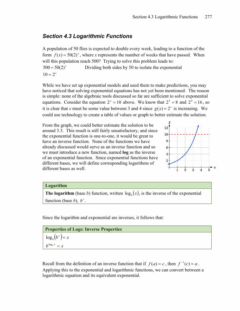
Section 4.3 Logarithmic Functions A population of 50 flies is expected to double every week, leading to a function of the form xxf )2(50)( = , where x represents the number of weeks that have passed. When will this population reach 500? Trying to solve this problem leads to: 500 50(2)x= Dividing both sides by 50 to isolate the exponential 10 2x= While we have set up exponential models and used them to make predictions, you may have noticed that solving exponential equations has not yet been mentioned. The reason is simple: none of the algebraic tools discussed so far are sufficient to solve exponential equations. Consider the equation 102 =x above. We know that 823 = and 1624 = , so it is clear that x must be some value between 3 and 4 since ( ) 2xg x = is increasing. We could use technology to create a table of values or graph to better estimate the solution. From the graph, we could better estimate the solution to be around 3.3. This result is still fairly unsatisfactory, and since the exponential function is one-to-one, it would be great to have an inverse function. None of the functions we have already discussed would serve as an inverse function and so we must introduce a new function, named log as the inverse of an exponential function. Since exponential functions have different bases, we will define corresponding logarithms of different bases as well.

Logarithm The logarithm (base b) function, written ( )xblog , is the inverse of the exponential function (base b), xb .

Since the logarithm and exponential are inverses, it follows that:

Properties of Logs: Inverse Properties

( ) xb xb =log

xb xb =log Recall from the definition of an inverse function that if caf =)( , then acf =− )(1 . Applying this to the exponential and logarithmic functions, we can convert between a logarithmic equation and its equivalent exponential.

Chapter 4 278

Logarithm Equivalent to an Exponential

The statement cba = is equivalent to the statement acb =)(log . Alternatively, we could show this by starting with the exponential function ac b= , then taking the log base b of both sides, giving log ( ) log a

b bc b= . Using the inverse property of logs, we see that log ( )b c a= . Since log is a function, it is most correctly written as )(log cb , using parentheses to denote function evaluation, just as we would with f(c). However, when the input is a single variable or number, it is common to see the parentheses dropped and the expression written as cblog . Example 1

Write these exponential equations as logarithmic equations:

a) 823 = b) 2552 = c) 10000

110 4 =−

a) 823 = is equivalent to 3)8(log2 = b) 2552 = is equivalent to 2)25(log5 =

c) 4 11010000

− = is equivalent to 101log 4

10000 = −

Example 2

Write these logarithmic equations as exponential equations:

a) ( )216log6 = b) ( ) 29log3 =

a) ( )216log6 = is equivalent to 66 2/1 =

b) ( ) 29log3 = is equivalent to 932 = Try it Now 1. Write the exponential equation 1642 = as a logarithmic equation.


By establishing the relationship between exponential and logarithmic functions, we can now solve basic logarithmic and exponential equations by rewriting. Example 3

Solve ( ) 2log4 =x for x. By rewriting this expression as an exponential, x=24 , so x = 16.

Example 4

Solve 102 =x for x. By rewriting this expression as a logarithm, we get )10(log2=x .

While this does define a solution, and an exact solution at that, you may find it somewhat unsatisfying since it is difficult to compare this expression to the decimal estimate we made earlier. Also, giving an exact expression for a solution is not always useful – often we really need a decimal approximation to the solution. Luckily, this is a task calculators and computers are quite adept at. Unluckily for us, most calculators and computers will only evaluate logarithms of two bases. Happily, this ends up not being a problem, as we’ll see briefly.

Common and Natural Logarithms The common log is the logarithm with base 10, and is typically written )log(x . The natural log is the logarithm with base e, and is typically written )ln(x .

Example 5

Evaluate )1000log( using the definition of the common log. To evaluate )1000log( , we can let

)1000log(=x , then rewrite into exponential form using the common log base of 10:

100010 =x . From this, we might recognize that 1000 is the cube of 10, so x = 3. We also can use the inverse property of logs to write ( ) 310log 3

10 = .

Values of the common log number number as

exponential log(number)

1000 103 3 100 102 2 10 101 1 1 100 0 0.1 10-1 -1 0.01 10-2 -2 0.001 10-3 -3

Chapter 4 280

Try it Now 2. Evaluate )1000000log( .

Example 6

Evaluate ( )eln . We can rewrite ( )eln as ( )2/1ln e . Since ln is a log base e, we can use the inverse

property for logs: ( ) ( )21logln 2/12/1 == ee e .

Example 7

Evaluate log(500) using your calculator or computer. Using a computer, we can evaluate 69897.2)500log( ≈

To utilize the common or natural logarithm functions to evaluate expressions like

)10(log2 , we need to establish some additional properties.

Properties of Logs: Exponent Property

( ) ( )ArA br

b loglog = To show why this is true, we offer a proof:

Since the logarithmic and exponential functions are inverses, Ab Ab =log . Raising both sides to the r power, we get ( )rAr bbA log= .

Utilizing the exponential rule that states ( )qp pqx x= , ( ) ArrAr bb bbA loglog ==

Taking the log of both sides, ( ) ( )Arb

rb

bbA logloglog = Utilizing the inverse property on the right side yields the result: ( ) ArA b

rb loglog =

Example 8

Rewrite ( )25log3 using the exponent property for logs. Since 25 = 52,

( ) ( ) ( )5log25log25log 32

33 ==


Example 9 Rewrite )ln(4 x using the exponent property for logs. Using the property in reverse, ( )4ln)ln(4 xx = .

Try it Now

3. Rewrite using the exponent property for logs:

2

1lnx

.

The exponent property allows us to find a method for changing the base of a logarithmic expression.

Properties of Logs: Change of Base

( ))(log)(log

logbA

Ac

cb =

Proof:

Let ( ) xAb =log . Rewriting as an exponential gives Ab x = . Taking the log base c of both sides of this equation gives Ab c

xc loglog = ,

Now utilizing the exponent property for logs on the left side, Abx cc loglog =

Dividing, we obtain bA

xc

c

loglog

= . Replacing our original expression for x,

bA

Ac

cb log

loglog =

With this change of base formula, we can finally find a good decimal approximation to our question from the beginning of the section. Example 10

Evaluate )10(log2 using the change of base formula. According to the change of base formula, we can rewrite the log base 2 as a logarithm of any other base. Since our calculators can evaluate the natural log, we might choose to use the natural logarithm, which is the log base e:

Chapter 4 282

2ln10ln

2log10log

10log2 ==e

e

Using our calculators to evaluate this,

3219.369315.030259.2

2ln10ln

≈≈

This finally allows us to answer our original question – the population of flies we discussed at the beginning of the section will take 3.32 weeks to grow to 500.

Example 11

Evaluate )100(log5 using the change of base formula. We can rewrite this expression using any other base. If our calculators are able to evaluate the common logarithm, we could rewrite using the common log, base 10.

861.269897.0

25log

100log)100(log

10

105 =≈=

While we can solve the basic exponential equation 102 =x by rewriting in logarithmic form and then using the change of base formula to evaluate the logarithm, the proof of the change of base formula illuminates an alternative approach to solving exponential equations.

Solving exponential equations: 1. Isolate the exponential expressions when possible 2. Take the logarithm of both sides 3. Utilize the exponent property for logarithms to pull the variable out of the

exponent 4. Use algebra to solve for the variable.

Example 12

Solve 102 =x for x. Using this alternative approach, rather than rewrite this exponential into logarithmic form, we will take the logarithm of both sides of the equation. Since we often wish to evaluate the result to a decimal answer, we will usually utilize either the common log or natural log. For this example, we’ll use the natural log:


( ) )10ln(2ln =x Utilizing the exponent property for logs, ( ) )10ln(2ln =x Now dividing by ln(2),

( ) 3219.32ln

)10ln(≈=x

Notice that this result matches the result we found using the change of base formula.

Example 13

In the first section, we predicted the population (in billions) of India t years after 2008 by using the function ttf )0134.01(14.1)( += . If the population continues following this trend, when will the population reach 2 billion? We need to solve for time t so that f(t) = 2.

t)0134.1(14.12 = Divide by 1.14 to isolate the exponential expression t0134.1

14.12

= Take the logarithm of both sides of the equation

( )t0134.1ln14.12ln =

Apply the exponent property on the right side

( )0134.1ln14.12ln t=

Divide both sides by ln(1.0134)

( ) 23.420134.1ln

14.12ln

≈

=t years

If this growth rate continues, the model predicts the population of India will reach 2 billion about 42 years after 2008, or approximately in the year 2050.

Try it Now 4. Solve 10)93.0(5 =x .

Example 14

Solve 2)07.1(5 3 =t To start, we want to isolate the exponential part of the expression, the t3)07.1( , so it is alone on one side of the equation. Then we can use the log to solve the equation. We can use any base log; this time we’ll use the common log.

Chapter 4 284

2)07.1(5 3 =t Divide both sides by 5 to isolate the exponential

52)07.1( 3 =t Take the log of both sides.

( )

=

52log)07.1(log 3t Use the exponent property for logs

( )

=

52log07.1log3t Divide by ( )07.1log3 on both sides

( )( ) ( )07.1log3

52log

07.1log307.1log3

=t Simplify and evaluate

( ) 5143.407.1log3

52log

−≈

=t

Note that when entering that expression on your calculator, be sure to put parentheses around the whole denominator to ensure the proper order of operations: log(2/5)/(3*log(1.07))

In addition to solving exponential equations, logarithmic expressions are common in many physical situations. Example 15

In chemistry, pH is a measure of the acidity or basicity of a liquid. The pH is related to the concentration of hydrogen ions, [H+], measured in moles per liter, by the equation

( )logpH H + = − .

If a liquid has concentration of 0.0001 moles per liber, determine the pH. Determine the hydrogen ion concentration of a liquid with pH of 7. To answer the first question, we evaluate the expression ( )0001.0log− . While we could use our calculators for this, we do not really need them here, since we can use the inverse property of logs:

( ) ( ) 4)4(10log0001.0log 4 =−−=−=− − To answer the second question, we need to solve the equation ( )7 log H + = − . Begin

by isolating the logarithm on one side of the equation by multiplying both sides by -1:

( )7 log H + − = . Rewriting into exponential form yields the answer: 710 0.0000001H + − = = moles per liter.


Logarithms also provide us a mechanism for finding continuous growth models for exponential growth given two data points. Example 15

A population grows from 100 to 130 in 2 weeks. Find the continuous growth rate. Measuring t in weeks, we are looking for an equation rtaetP =)( so that P(0) = 100 and P(2) = 130. Using the first pair of values,

0100 rae ⋅= , so a = 100. Using the second pair of values,

2130 100 re ⋅= Divide by 100 2

100130 re= Take the natural log of both sides

( )2ln)3.1ln( re= Use the inverse property of logs

1312.02

)3.1ln(2)3.1ln(

≈=

=

r

r

This population is growing at a continuous rate of 13.12% per week.

In general, we can relate the standard form of an exponential with the continuous growth form by noting (using k to represent the continuous growth rate to avoid the confusion of using r in two different ways in the same formula):

kxx aera =+ )1( kxx er =+ )1(

ker =+1

Converting Between Periodic to Continuous Growth Rate In the equation xraxf )1()( += , r is the periodic growth rate, the percent growth each time period (weekly growth, annual growth, etc.). In the equation kxaexf =)( , k is the continuous growth rate. You can convert between these using: ker =+1 .

Remember that the continuous growth rate k represents the nominal growth rate before accounting for the effects of continuous compounding, while r represents the actual percent increase in one time unit (one week, one year, etc.).

Chapter 4 286

Example 16

A company’s sales can be modeled by the function tetS 12.05000)( = , with t measured in years. Find the annual growth rate. Noting that ker =+1 , then 1275.0112.0 =−= er , so the annual growth rate is 12.75%. The sales function could also be written in the form ttS )1275.01(5000)( += .

Important Topics of this Section The Logarithmic function as the inverse of the exponential function Writing logarithmic & exponential expressions Properties of logs Inverse properties Exponential properties Change of base Common log Natural log Solving exponential equations Converting between periodic and continuous growth rate.

Try it Now Answers 1. ( ) 4log24log216log 4

244 ===

2. ( ) ( ) 610log1000000log 6 ==

3. ( ) )ln(2ln1ln 22 xx

x−==

−

4. 10)93.0(5 =x

2)93.0( =x ( ) ( )2ln93.0ln =x ( ) ( )2ln93.0ln =x

5513.9)93.0ln(

)2ln(−≈


Section 4.3 Exercises Rewrite each equation in exponential form 1. 4log ( )q m= 2. 3log ( )t k= 3. log ( )a b c= 4. log ( )p z u=

( )5. log v t= 6. ( )log r s= 7. ( )ln w n= 8. ( )ln x y= Rewrite each equation in logarithmic form. 9. 4x y= 10. 5y x= 11. dc k= 12. zn L=

13. 10a b= 14. 10 p v= 15. ke h= 16. ye x=

Solve for x. 17. ( )3log 2x = 18. 4log ( ) 3x = 19. 2log ( ) 3x = − 20. 5log ( ) 1x = −

21. ( )log 3x = 22. ( )log 5x = 23. ( )ln 2x = 24. ( )ln 2x = −

Simplify each expression using logarithm properties.

25. ( )5log 25 26. ( )2log 8 27. 31log27

28. 61log36

29. ( )6log 6 30. ( )35log 5 31. ( )log 10,000 32. ( )log 100

33. ( )log 0.001 34. ( )log 0.00001 35. ( )2ln e− 36. ( )3ln e

Evaluate using your calculator. 37. ( )log 0.04 38. ( )log 1045 39. ( )ln 15 40. ( )ln 0.02 Solve each equation for the variable.

41. 5 14x = 42. 3 23x = 43. 1715

x = 44. 134

x =

45. 5 17xe = 46. 3 12xe = 47. 4 53 38x− = 48. 2 34 44x− =

49. ( )1000 1.03 5000t = 50. ( )200 1.06 550t =

51. ( )33 1.04 8t = 52. ( )42 1.08 7t =

53. 0.1250 10te− = 54. 0.0310 4te− =

55. 110 8 52

x − =

56. 1100 100 704

x − =

Chapter 4 288

Convert the equation into continuous growth form, ( ) ktf t ae= .

57. ( ) ( )300 0.91 tf t = 58. ( ) ( )120 0.07 tf t =

59. ( ) ( )10 1.04 tf t = 60. ( ) ( )1400 1.12 tf t =

Convert the equation into annual growth form, ( ) tf t ab= .

61. ( ) 0.061 50 tf t e= 62. ( ) 0.12100 tf t e=

63. ( ) 0.01250 tf t e−= 64. ( ) 0.8580 tf t e−=

65. The population of Kenya was 39.8 million in 2009 and has been growing by about

2.6% each year. If this trend continues, when will the population exceed 45 million?

66. The population of Algeria was 34.9 million in 2009 and has been growing by about 1.5% each year. If this trend continues, when will the population exceed 45 million?

67. The population of Seattle grew from 563,374 in 2000 to 608,660 in 2010. If the population continues to grow exponentially at the same rate, when will the population exceed 1 million people?

68. The median household income (adjusted for inflation) in Seattle grew from $42,948 in 1990 to $45,736 in 2000. If it continues to grow exponentially at the same rate, when will median income exceed $50,000?

69. A scientist begins with 100 mg of a radioactive substance. After 4 hours, it has decayed to 80 mg. How long after the process began will it take to decay to 15 mg?

70. A scientist begins with 100 mg of a radioactive substance. After 6 days, it has decayed to 60 mg. How long after the process began will it take to decay to 10 mg?

71. If $1000 is invested in an account earning 3% compounded monthly, how long will it take the account to grow in value to $1500?

72. If $1000 is invested in an account earning 2% compounded quarterly, how long will it take the account to grow in value to $1300?

Section 4.4 Logarithmic Properties 289

Section 4.4 Logarithmic Properties In the previous section, we derived two important properties of logarithms, which allowed us to solve some basic exponential and logarithmic equations.

Properties of Logs Inverse Properties:

( ) xb xb =log

xb xb =log Exponential Property:

( ) ( )ArA br

b loglog =

Change of Base:

( ))(log)(log

logbA

Ac

cb =

While these properties allow us to solve a large number of problems, they are not sufficient to solve all problems involving exponential and logarithmic equations.

Properties of Logs Sum of Logs Property:

( ) ( ) )(logloglog ACCA bbb =+

Difference of Logs Property:

( ) ( )

=−

CACA bbb logloglog

It’s just as important to know what properties logarithms do not satisfy as to memorize the valid properties listed above. In particular, the logarithm is not a linear function, which means that it does not distribute: log(A + B) ≠ log(A) + log(B). To help in this process we offer a proof to help solidify our new rules and show how they follow from properties you’ve already seen.

Chapter 4 290

Let ( )Aa blog= and ( )Cc blog= . By definition of the logarithm, Aba = and Cbc = . Using these expressions, cabbAC = Using exponent rules on the right, cabAC += Taking the log of both sides, and utilizing the inverse property of logs,

( ) ( ) cabAC cabb +== +loglog

Replacing a and c with their definition establishes the result ( ) CAAC bbb logloglog +=

The proof for the difference property is very similar. With these properties, we can rewrite expressions involving multiple logs as a single log, or break an expression involving a single log into expressions involving multiple logs. Example 1

Write ( ) ( ) ( )2log8log5log 333 −+ as a single logarithm. Using the sum of logs property on the first two terms,

( ) ( ) ( ) ( )40log85log8log5log 3333 =⋅=+ This reduces our original expression to ( ) ( )2log40log 33 − Then using the difference of logs property,

( ) ( ) ( )20log240log2log40log 3333 =

=−

Example 2

Evaluate ( ) ( )4log5log2 + without a calculator by first rewriting as a single logarithm. On the first term, we can use the exponent property of logs to write

( ) ( ) ( )25log5log5log2 2 == With the expression reduced to a sum of two logs, ( ) ( )4log25log + , we can utilize the sum of logs property

( ) ( ) )100log()254log(4log25log =⋅=+ Since 100 = 102, we can evaluate this log without a calculator:

( ) 210log)100log( 2 ==


Try it Now 1. Without a calculator evaluate by first rewriting as a single logarithm:

( ) ( )4log8log 22 +

Example 3

Rewrite

7

ln4 yx as a sum or difference of logs

First, noticing we have a quotient of two expressions, we can utilize the difference property of logs to write

( ) )7ln(ln7

ln 44

−=

yxyx

Then seeing the product in the first term, we use the sum property ( ) ( ) )7ln()ln(ln)7ln(ln 44 −+=− yxyx

Finally, we could use the exponent property on the first term ( ) )7ln()ln()ln(4)7ln()ln(ln 4 −+=−+ yxyx

Interestingly, solving exponential equations was not the reason logarithms were originally developed. Historically, up until the advent of calculators and computers, the power of logarithms was that these log properties reduced multiplication, division, roots, or powers to be evaluated using addition, subtraction, division and multiplication, respectively, which are much easier to compute without a calculator. Large books were published listing the logarithms of numbers, such as in the table to the right. To find the product of two numbers, the sum of log property was used. Suppose for example we didn’t know the value of 2 times 3. Using the sum property of logs:

)3log()2log()32log( +=⋅ Using the log table,

7781513.04771213.03010300.0)3log()2log()32log( =+=+=⋅ We can then use the table again in reverse, looking for 0.7781513 as an output of the logarithm. From that we can determine:

)6log(7781513.0)32log( ==⋅ . By using addition and the table of logs, we were able to determine 632 =⋅ .

value log(value) 1 0.0000000 2 0.3010300 3 0.4771213 4 0.6020600 5 0.6989700 6 0.7781513 7 0.8450980 8 0.9030900 9 0.9542425

10 1.0000000

Chapter 4 292

Likewise, to compute a cube root like 3 8

( ) )2log(3010300.0)9030900.0(31)8log(

318log)8log( 3/13 ======

So 283 = . Although these calculations are simple and insignificant, they illustrate the same idea that was used for hundreds of years as an efficient way to calculate the product, quotient, roots, and powers of large and complicated numbers, either using tables of logarithms or mechanical tools called slide rules. These properties still have other practical applications for interpreting changes in exponential and logarithmic relationships. Example 4

Recall that in chemistry, ( )logpH H + = − . If the concentration of hydrogen ions in a

liquid is doubled, what is the affect on pH? Suppose C is the original concentration of hydrogen ions, and P is the original pH of the liquid, so ( )CP log−= . If the concentration is doubled, the new concentration is 2C. Then the pH of the new liquid is

( )CpH 2log−= Using the sum property of logs,

( ) ( ) )log()2log()log()2log(2log CCCpH −−=+−=−= Since ( )CP log−= , the new pH is

301.0)2log( −=−= PPpH When the concentration of hydrogen ions is doubled, the pH decreases by 0.301.

Log properties in solving equations The logarithm properties often arise when solving problems involving logarithms. First, we’ll look at a simpler log equation. Example 5

Solve 3)62log( =−x . To solve for x, we need to get it out from inside the log function. There are two ways we can approach this.


Method 1: Rewrite as an exponential. Recall that since the common log is base 10, BA =)log( can be rewritten as the exponential AB =10 . Likewise, 3)62log( =−x can be rewritten in exponential form as

62103 −= x Method 2: Exponentiate both sides. If BA = , then BA 1010 = . Using this idea, since 3)62log( =−x , then 3)62log( 1010 =−x . Use the inverse property of logs to rewrite the left side and get 31062 =−x . Using either method, we now need to solve 31062 =−x . Evaluate 310 to get

100062 =−x Add 6 to both sides 10062 =x Divide both sides by 2

503=x Occasionally the solving process will result in extraneous solutions – answers that are outside the domain of the original equation. In this case, our answer looks fine.

Example 6

Solve 2)log()2550log( =−+ xx . In order to rewrite in exponential form, we need a single logarithmic expression on the left side of the equation. Using the difference property of logs, we can rewrite the left side:

22550log =

+

xx

Rewriting in exponential form reduces this to an algebraic equation:

100102550 2 ==+x

x Multiply both sides by x

xx 1002550 =+ Combine like terms x5025 = Divide by 50

21

5025

==x

Checking this answer in the original equation, we can verify there are no domain issues, and this answer is correct.

Try it Now 2. Solve )2log(1)4log( 2 ++=− xx .

Chapter 4 294

Example 7 Solve )144ln()1ln()2ln( +=+++ xxx .

)144ln()1ln()2ln( +=+++ xxx Use the sum of logs property on the right ( ) )144ln()1)(2(ln +=++ xxx Expand ( ) )144ln(23ln 2 +=++ xxx

We have a log on both side of the equation this time. Rewriting in exponential form would be tricky, so instead we can exponentiate both sides.

( ) )134ln(23ln 2 +++ = xxx ee Use the inverse property of logs 144232 +=++ xxx Move terms to one side

0122 =−− xx Factor 0)3)(4( =−+ xx

x = −4 or x = 3. Checking our answers, notice that evaluating the original equation at x = −4 would result in us evaluating )2ln(− , which is undefined. That answer is outside the domain of the original equation, so it is an extraneous solution and we discard it. There is one solution: x = 3.

More complex exponential equations can often be solved in more than one way. In the following example, we will solve the same problem in two ways – one using logarithm properties, and the other using exponential properties. Example 8a

In 2008, the population of Kenya was approximately 38.8 million, and was growing by 2.64% each year, while the population of Sudan was approximately 41.3 million and growing by 2.24% each year2. If these trends continue, when will the population of Kenya match that of Sudan? We start by writing an equation for each population in terms of t, the number of years after 2008.

( ) 38.8(1 0.0264)( ) 41.3(1 0.0224)

t

t

Kenya tSudan t

= +

= +

To find when the populations will be equal, we can set the equations equal 38.8(1.0264) 41.3(1.0224)t t=

2 World Bank, World Development Indicators, as reported on http://www.google.com/publicdata, retrieved August 24, 2010

http://www.google.com/publicdata


For our first approach, we take the log of both sides of the equation. ( ) ( )log 38.8(1.0264) log 41.3(1.0224)t t=

Utilizing the sum property of logs, we can rewrite each side,

( ) ( )log(38.8) log 1.0264 log(41.3) log 1.0224t t+ = + Then utilizing the exponent property, we can pull the variables out of the exponent

( ) ( )log(38.8) log 1.0264 log(41.3) log 1.0224t t+ = + Moving all the terms involving t to one side of the equation and the rest of the terms to the other side,

( ) ( )log 1.0264 log 1.0224 log(41.3) log(38.8)t t− = − Factoring out the t on the left,

( ) ( )( )log 1.0264 log 1.0224 log(41.3) log(38.8)t − = − Dividing to solve for t

( ) ( )log(41.3) log(38.8) 15.991

log 1.0264 log 1.0224t −= ≈

−years until the populations will be equal.

Example 8b

Solve the problem above by rewriting before taking the log. Starting at the equation 38.8(1.0264) 41.3(1.0224)t t= Divide to move the exponential terms to one side of the equation and the constants to the other side 1.0264 41.31.0224 38.8

t

t =

Using exponent rules to group on the left,

1.0264 41.31.0224 38.8

t =

Taking the log of both sides

1.0264 41.3log log1.0224 38.8

t =

Chapter 4 296

Utilizing the exponent property on the left, 1.0264 41.3log log1.0224 38.8

t =

Dividing gives

41.3log38.8 15.991

1.0264log1.0224

t

= ≈

years

While the answer does not immediately appear identical to that produced using the previous method, note that by using the difference property of logs, the answer could be rewritten:

41.3loglog(41.3) log(38.8)38.8

1.0264 log(1.0264) log(1.0224)log1.0224

t

− = =

−

While both methods work equally well, it often requires fewer steps to utilize algebra before taking logs, rather than relying solely on log properties. Try it Now 3. Tank A contains 10 liters of water, and 35% of the water evaporates each week. Tank

B contains 30 liters of water, and 50% of the water evaporates each week. In how many weeks will the tanks contain the same amount of water?

Important Topics of this Section Inverse Exponential Change of base Sum of logs property Difference of logs property Solving equations using log rules


Try it Now Answers 1. ( ) ( ) ( ) 52log32log48log 5

222 ===⋅ 2. )2log(1)4log( 2 ++=− xx Move both logs to one side

( ) ( ) 12log4log 2 =+−− xx Use the difference property of logs

124log

2

=

+−

xx Factor

12

)2)(2(log =

+−+

xxx Simplify

( ) 12log =−x Rewrite as an exponential 2101 −= x Add 2 to both sides

12=x 3. Tank A: ttA )35.01(10)( −= . Tank B: ttB )50.01(30)( −=

Solving A(t) = B(t), tt )5.0(30)65.0(10 = Using the method from Example 8b

1030

)5.0()65.0(=t

t

Regroup

35.065.0

=

t

Simplify

( ) 33.1 =t Take the log of both sides ( )( ) ( )3log3.1log =t Use the exponent property of logs ( ) ( )3log3.1log =t Divide and evaluate

( )( ) 1874.4

3.1log3log

≈=t weeks

Chapter 4 298

Section 4.4 Exercises Simplify to a single logarithm, using logarithm properties. 1. ( ) ( )3 3log 28 log 7− 2. ( ) ( )3 3log 32 log 4−

3. 31log7

−

4. 41log5

−

5. ( )3 31log log 50

10 +

6. ( )4 4log 3 log (7)+

7. ( )71 log 83

8. ( )51 log 362

9. ( ) ( )4 5log 2 log 3x x+ 10. ( ) ( )2 3ln 4 ln 3x x+

11. ( ) ( )9 2ln 6 ln 3x x− 12. ( ) ( )4log 12 log 4x x−

13. ( ) ( )2log 3log 1x x+ + 14. ( ) ( )23log 2logx x+

15. ( ) ( ) ( )1log log 3log2

x y z− + 16. ( ) ( ) ( )12log log log3

x y z+ −

Use logarithm properties to expand each expression.

17. 15 13

19log x yz

18. 2 3

5log a bc

19. 2

4 5ln ab c

−

−

20. 2 3

5ln a bc

−

−

21. ( )3 4log x y− 22. ( )3 2log x y−

23. ln1

yyy

−

24. 2

ln1

xx

−

25. ( )2 3 2 53log x y x y 26. ( )3 4 3 97log x y x y


Solve each equation for the variable. 27. 4 7 9 64 3x x− −= 28. 2 5 3 72 7x x− −=

29. ( ) ( )17 1.14 19 1.16x x= 30. ( ) ( )20 1.07 8 1.13x x=

31. 0.12 0.085 10t te e= 32. 0.09 0.143 t te e=

33. ( )2log 7 6 3x + = 34. 3log (2 4) 2x + =

35. ( )2ln 3x 3 1+ = 36. ( )4ln 5 5 2x + =

37. ( )3log 2x = 38. ( )5log 3x =

39. ( ) ( )log log 3 3x x+ + = 40. ( ) ( )log 4 log 9x x+ + =

41. ( ) ( )log 4 log 3 1x x+ − + = 42. ( ) ( )log 5 log 2 2x x+ − + =

43. ( )26 6log log ( 1) 1x x− + = 44. 2

3 3log ( ) log ( 2) 5x x− + =

45. ( ) ( ) ( )log 12 log log 12x x+ = + 46. ( ) ( ) ( )log 15 log log 15x x+ = +

47. ( ) ( ) ( )ln ln 3 ln 7x x x+ − = 48. ( ) ( ) ( )ln ln 6 ln 6x x x+ − =

Chapter 4 300

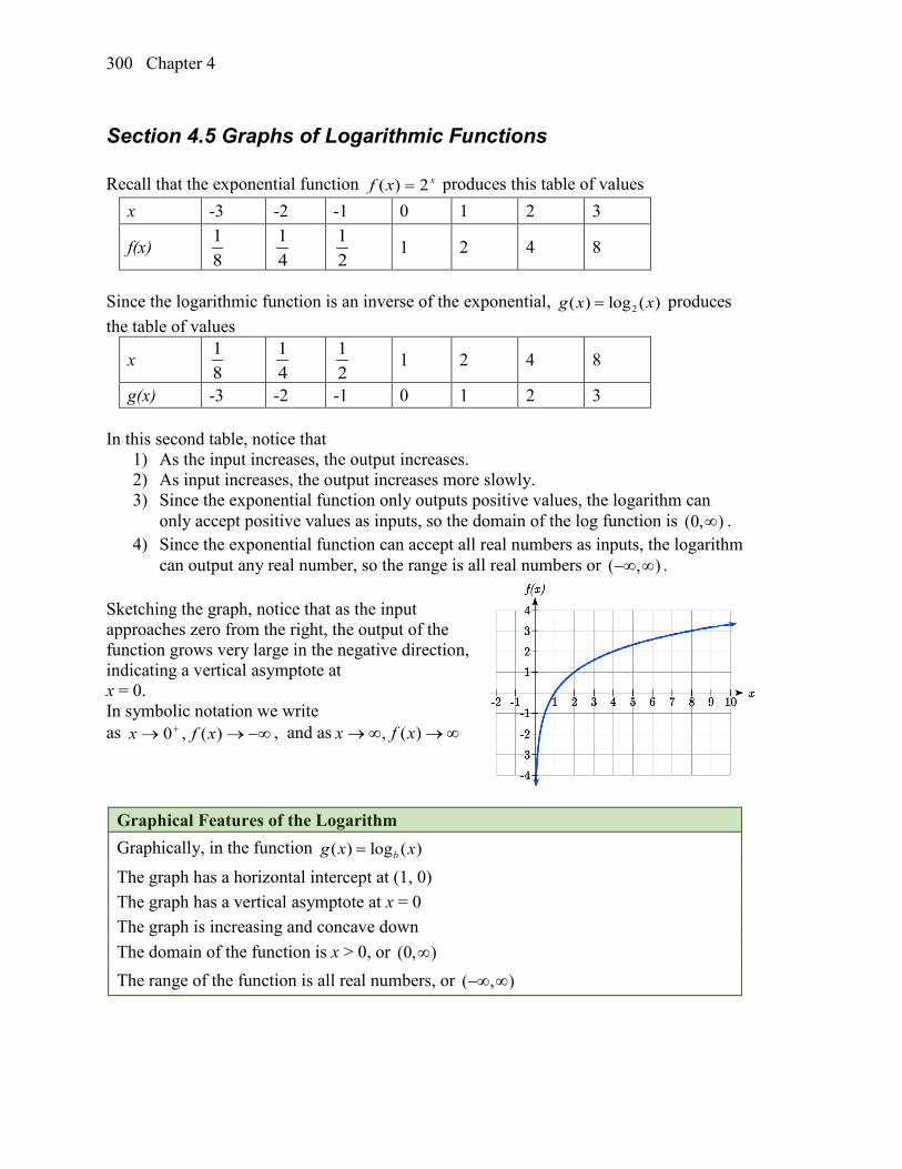
Section 4.5 Graphs of Logarithmic Functions Recall that the exponential function xxf 2)( = produces this table of values

x -3 -2 -1 0 1 2 3

f(x) 81

41

21 1 2 4 8

Since the logarithmic function is an inverse of the exponential, 2( ) log ( )g x x= produces the table of values

x 81

41

21 1 2 4 8

g(x) -3 -2 -1 0 1 2 3 In this second table, notice that

1) As the input increases, the output increases. 2) As input increases, the output increases more slowly. 3) Since the exponential function only outputs positive values, the logarithm can

only accept positive values as inputs, so the domain of the log function is ),0( ∞ . 4) Since the exponential function can accept all real numbers as inputs, the logarithm

can output any real number, so the range is all real numbers or ),( ∞−∞ . Sketching the graph, notice that as the input approaches zero from the right, the output of the function grows very large in the negative direction, indicating a vertical asymptote at x = 0. In symbolic notation we write as −∞→→ + )(,0 xfx , and as ∞→∞→ )(, xfx

Graphical Features of the Logarithm Graphically, in the function ( ) log ( )bg x x=

The graph has a horizontal intercept at (1, 0) The graph has a vertical asymptote at x = 0 The graph is increasing and concave down The domain of the function is x > 0, or ),0( ∞ The range of the function is all real numbers, or ),( ∞−∞

Section 4.5 Graphs of Logarithmic Functions 301

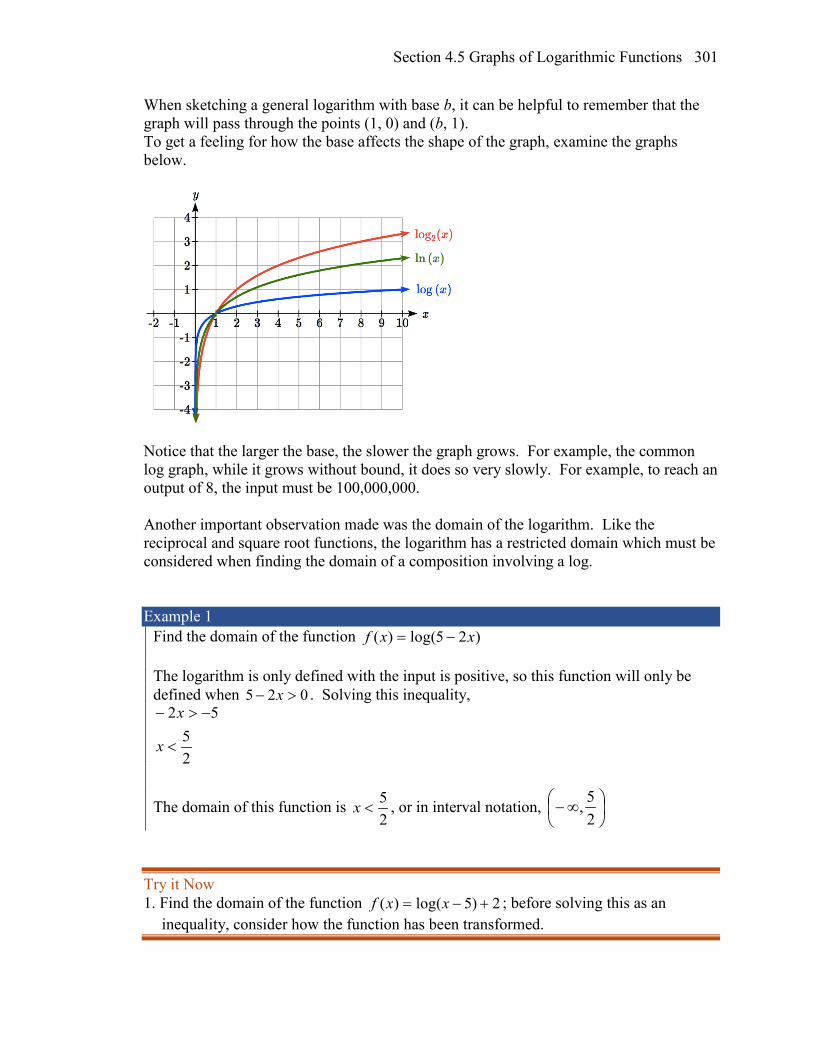
When sketching a general logarithm with base b, it can be helpful to remember that the graph will pass through the points (1, 0) and (b, 1). To get a feeling for how the base affects the shape of the graph, examine the graphs below.

Notice that the larger the base, the slower the graph grows. For example, the common log graph, while it grows without bound, it does so very slowly. For example, to reach an output of 8, the input must be 100,000,000. Another important observation made was the domain of the logarithm. Like the reciprocal and square root functions, the logarithm has a restricted domain which must be considered when finding the domain of a composition involving a log. Example 1

Find the domain of the function )25log()( xxf −= The logarithm is only defined with the input is positive, so this function will only be defined when 025 >− x . Solving this inequality,

25

52

<

−>−

x

x

The domain of this function is 25

<x , or in interval notation,

∞−

25,

Try it Now 1. Find the domain of the function 2)5log()( +−= xxf ; before solving this as an

inequality, consider how the function has been transformed.

Chapter 4 302

Transformations of the Logarithmic Function Transformations can be applied to a logarithmic function using the basic transformation techniques, but as with exponential functions, several transformations result in interesting relationships.

First recall the change of base property tells us that xbb

xx c

cc

cb log

log1

loglog

log ==

From this, we can see that xblog is a vertical stretch or compression of the graph of the xclog graph. This tells us that a vertical stretch or compression is equivalent to a change

of base. For this reason, we typically represent all graphs of logarithmic functions in terms of the common or natural log functions. Next, consider the effect of a horizontal compression on the graph of a logarithmic function. Considering )log()( cxxf = , we can use the sum property to see

)log()log()log()( xccxxf +== Since log(c) is a constant, the effect of a horizontal compression is the same as the effect of a vertical shift. Example 2

Sketch )ln()( xxf = and 2)ln()( += xxg . Graphing these,

Note that this vertical shift could also be written as a horizontal compression, since

)ln()ln()ln(2)ln()( 22 xeexxxg =+=+= . While a horizontal stretch or compression can be written as a vertical shift, a horizontal reflection is unique and separate from vertical shifting. Finally, we will consider the effect of a horizontal shift on the graph of a logarithm.


Example 3 Sketch a graph of )2ln()( += xxf . This is a horizontal shift to the left by 2 units. Notice that none of our logarithm rules allow us rewrite this in another form, so the effect of this transformation is unique. Shifting the graph,

Notice that due to the horizontal shift, the vertical asymptote shifted to x = -2, and the domain shifted to ( 2, )− ∞ .

Combining these transformations, Example 4

Sketch a graph of )2log(5)( +−= xxf . Factoring the inside as ))2(log(5)( −−= xxf reveals that this graph is that of the common logarithm, horizontally reflected, vertically stretched by a factor of 5, and shifted to the right by 2 units. The vertical asymptote will be shifted to x = 2, and the graph will have domain ( , 2)∞ . A rough sketch can be created by using the vertical asymptote along with a couple points on the graph, such as

5)10log(5)2)8(log(5)8(0)1log(5)21log(5)1(

==+−−=−==+−=

ff

Chapter 4 304

Try it Now 2. Sketch a graph of the function 1)2log(3)( +−−= xxf .

Transformations of Logs Any transformed logarithmic function can be written in the form

( ) log( )f x a x b k= − + , or ( )( )( ) logf x a x b k= − − + if horizontally reflected,

where x = b is the vertical asymptote.

Example 5

Find an equation for the logarithmic function graphed. This graph has a vertical asymptote at x = –2 and has been vertically reflected. We do not know yet the vertical shift (equivalent to horizontal stretch) or the vertical stretch (equivalent to a change of base). We know so far that the equation will have form

kxaxf ++−= )2log()( It appears the graph passes through the points (–1, 1) and (2, –1). Substituting in (–1, 1),

kka

ka

=+−=

++−−=

1)1log(1

)21log(1

Next, substituting in (2, –1),

)4log(2

)4log(21)22log(1

=

−=−++−=−

a

aa

This gives us the equation 1)2log()4log(

2)( ++−= xxf .

This could also be written as 4( ) 2 log ( 2) 1f x x= − + + .


Try it Now 3. Write an equation for the function graphed here. Flashback 4. Write the domain and range of the function graphed in Example 5, and describe its

long run behavior.

Important Topics of this Section Graph of the logarithmic function (domain and range) Transformation of logarithmic functions Creating graphs from equations Creating equations from graphs

Try it Now and Flashback Answers 1. Domain: {x| x > 5}

2. 3. The graph is horizontally reflected and has a vertical asymptote at x = 3, giving form

( )( ) kxaxf +−−= 3log)( . Substituting in the point (2,0) gives ( )( ) ka +−−= 32log0 ,

simplifying to k = 0. Substituting in (-2,-2), ( )( )32log2 −−−=− a , so a=−

)5log(2 .

The equation is ( )( )3log)5log(

2)( −−−

= xxf or ( )( )3log2)( 5 −−−= xxf .

4. Domain: {x| x>-2}, Range: all real numbers; As ∞→−→ + )(,2 xfx and as

−∞→∞→ )(, xfx .

Chapter 4 306

Section 4.5 Exercises For each function, find the domain and the vertical asymptote. 1. ( ) ( )log 5f x x= − 2. ( ) ( )log 2f x x= +

3. ( ) ( )ln 3f x x= − 4. ( ) ( )ln 5f x x= −

5. ( ) ( )log 3 1f x x= + 6. ( ) ( )log 2 5f x x= +

7. ( ) ( )3log 2f x x= − + 8. ( ) ( )2log 1f x x= − +

Sketch a graph of each pair of functions. 9. ( ) ( ) ( ) ( )log , lnf x x g x x= = 10. ( ) ( ) ( )2 4log ( ), logf x x g x x= = Sketch each transformation. 11. ( ) ( )2logf x x= 12. ( ) ( )3lnf x x=

13. ( ) ( )lnf x x= − 14. ( ) ( )logf x x= −

15. ( ) 2log ( 2)f x x= + 16. ( ) ( )3log 4f x x= +

Find a formula for the transformed logarithm graph shown.

17. 18.


19. 20. Find a formula for the transformed logarithm graph shown.

21. 22.

23. 24.

Chapter 4 308

Section 4.6 Exponential and Logarithmic Models While we have explored some basic applications of exponential and logarithmic functions, in this section we explore some important applications in more depth. Radioactive Decay In an earlier section, we discussed radioactive decay – the idea that radioactive isotopes change over time. One of the common terms associated with radioactive decay is half-life.

Half Life The half-life of a radioactive isotope is the time it takes for half the substance to decay.

Given the basic exponential growth/decay equation tabth =)( , half-life can be found by

solving for when half the original amount remains; by solving tbaa )(21

= , or more

simply tb=21 . Notice how the initial amount is irrelevant when solving for half-life.

Example 1

Bismuth-210 is an isotope that decays by about 13% each day. What is the half-life of Bismuth-210? We were not given a starting quantity, so we could either make up a value or use an unknown constant to represent the starting amount. To show that starting quantity does not affect the result, let us denote the initial quantity by the constant a. Then the decay of Bismuth-210 can be described by the equation dadQ )87.0()( = . To find the half-life, we want to determine when the remaining quantity is half the

original: 12

a . Solving,

daa )87.0(21

= Divide by a,

d87.021= Take the log of both sides

( )d87.0log21log =

Use the exponent property of logs

Section 4.6 Exponential and Logarithmic Models 309

( )87.0log21log d=

Divide to solve for d

( )

1log2 4.977

log 0.87d

= ≈ days

This tells us that the half-life of Bismuth-210 is approximately 5 days.

Example 2

Cesium-137 has a half-life of about 30 years. If you begin with 200mg of cesium-137, how much will remain after 30 years? 60 years? 90 years? Since the half-life is 30 years, after 30 years, half the original amount, 100mg, will remain. After 60 years, another 30 years have passed, so during that second 30 years, another half of the substance will decay, leaving 50mg. After 90 years, another 30 years have passed, so another half of the substance will decay, leaving 25mg.

Example 3

Cesium-137 has a half-life of about 30 years. Find the annual decay rate. Since we are looking for an annual decay rate, we will use an equation of the form

tratQ )1()( += . We know that after 30 years, half the original amount will remain. Using this information

30)1(21 raa += Dividing by a

30)1(21 r+= Taking the 30th root of both sides

r+= 121

30 Subtracting one from both sides,

02284.0121

30 −≈−=r

This tells us cesium-137 is decaying at an annual rate of 2.284% per year.

Chapter 4 310

Try it Now 1. Chlorine-36 is eliminated from the body with a biological half-life of 10 days3. Find

the daily decay rate. Example 4

Carbon-14 is a radioactive isotope that is present in organic materials, and is commonly used for dating historical artifacts. Carbon-14 has a half-life of 5730 years. If a bone fragment is found that contains 20% of its original carbon-14, how old is the bone? To find how old the bone is, we first will need to find an equation for the decay of the carbon-14. We could either use a continuous or annual decay formula, but opt to use the continuous decay formula since it is more common in scientific texts. The half life tells us that after 5730 years, half the original substance remains. Solving for the rate,

5730

21 raea = Dividing by a

5730

21 re= Taking the natural log of both sides

( )5730ln21ln re=

Use the inverse property of logs on the right side

r573021ln =

Divide by 5730

000121.05730

21ln

−≈

=r

Now we know the decay will follow the equation taetQ 000121.0)( −= . To find how old the bone fragment is that contains 20% of the original amount, we solve for t so that Q(t) = 0.20a.

taea 000121.020.0 −= te 000121.020.0 −=

( )te 000121.0ln)20.0ln( −= t000121.0)20.0ln( −=

13301000121.0

)20.0ln(≈

−=t years

The bone fragment is about 13,300 years old.

3 http://www.ead.anl.gov/pub/doc/chlorine.pdf

http://www.ead.anl.gov/pub/doc/chlorine.pdf


Try it Now 2. In Example 2, we learned that Cesium-137 has a half-life of about 30 years. If you

begin with 200mg of cesium-137, will it take more or less than 230 years until only 1 milligram remains?

Doubling Time For decaying quantities, we asked how long it takes for half the substance to decay. For growing quantities we might ask how long it takes for the quantity to double.

Doubling Time The doubling time of a growing quantity is the time it takes for the quantity to double.

Given the basic exponential growth equation tabth =)( , doubling time can be found by solving for when the original quantity has doubled; by solving xbaa )(2 = , or more simply xb=2 . Like with decay, the initial amount is irrelevant when solving for doubling time. Example 5

Cancer cells sometimes increase exponentially. If a cancerous growth contained 300 cells last month and 360 cells this month, how long will it take for the number of cancer cells to double? Defining t to be time in months, with t = 0 corresponding to this month, we are given two pieces of data: this month, (0, 360), and last month, (-1, 300). From this data, we can find an equation for the growth. Using the form tabtC =)( , we know immediately a = 360, giving tbtC 360)( = . Substituting in (-1, 300),

2.1300360

360300

360300 1

==

=

= −

b

b

b

This gives us the equation ttC )2.1(360)( = To find the doubling time, we look for the time when we will have twice the original amount, so when C(t) = 2a.

Chapter 4 312

taa )2.1(2 = t)2.1(2 =

( ) ( )t2.1log2log = ( ) ( )2.1log2log t=

( )( ) 802.3

2.1log2log

≈=t months for the number of cancer cells to double.

Example 6

Use of a new social networking website has been growing exponentially, with the number of new members doubling every 5 months. If the site currently has 120,000 users and this trend continues, how many users will the site have in 1 year? We can use the doubling time to find a function that models the number of site users, and then use that equation to answer the question. While we could use an arbitrary a as we have before for the initial amount, in this case, we know the initial amount was 120,000. If we use a continuous growth equation, it would look like rtetN 120)( = , measured in thousands of users after t months. Based on the doubling time, there would be 240 thousand users after 5 months. This allows us to solve for the continuous growth rate:

5120240 re= 52 re=

r52ln =

1386.052ln≈=r

Now that we have an equation, tetN 1386.0120)( = , we can predict the number of users after 12 months:

140.633120)12( )12(1386.0 == eN thousand users. So after 1 year, we would expect the site to have around 633,140 users.

Try it Now 3. If tuition at a college is increasing by 6.6% each year, how many years will it take for

tuition to double?


Newton’s Law of Cooling When a hot object is left in surrounding air that is at a lower temperature, the object’s temperature will decrease exponentially, leveling off towards the surrounding air temperature. This "leveling off" will correspond to a horizontal asymptote in the graph of the temperature function. Unless the room temperature is zero, this will correspond to a vertical shift of the generic exponential decay function.

Newton’s Law of Cooling The temperature of an object, T, in surrounding air with temperature Ts will behave according to the formula

skt TaetT +=)(

Where t is time a is a constant determined by the initial temperature of the object k is a constant, the continuous rate of cooling of the object

While an equation of the form s

t TabtT +=)( could be used, the continuous growth form is more common. Example 7

A cheesecake is taken out of the oven with an ideal internal temperature of 165 degrees Fahrenheit, and is placed into a 35 degree refrigerator. After 10 minutes, the cheesecake has cooled to 150 degrees. If you must wait until the cheesecake has cooled to 70 degrees before you eat it, how long will you have to wait? Since the surrounding air temperature in the refrigerator is 35 degrees, the cheesecake’s temperature will decay exponentially towards 35, following the equation

35)( += ktaetT We know the initial temperature was 165, so 165)0( =T . Substituting in these values,

13035165

35165 0

=+=

+=

aaaek

Chapter 4 314

We were given another pair of data, 150)10( =T , which we can use to solve for k 35130150 10 += ke

0123.010130115ln

10130115ln

130115

130115

10

10

−=

=

=

=

=

k

k

e

e

k

k

Together this gives us the equation for cooling: 35130)( 0123.0 += − tetT . Now we can solve for the time it will take for the temperature to cool to 70 degrees.

3513070 0123.0 += − te te 0123.013035 −=

te 0123.0

13035 −=

t0123.013035ln −=

68.1060123.013035ln

≈−

=t

It will take about 107 minutes, or one hour and 47 minutes, for the cheesecake to cool. Of course, if you like your cheesecake served chilled, you’d have to wait a bit longer.

Try it Now 4. A pitcher of water at 40 degrees Fahrenheit is placed into a 70 degree room. One hour

later the temperature has risen to 45 degrees. How long will it take for the temperature to rise to 60 degrees?

Logarithmic Scales For quantities that vary greatly in magnitude, a standard scale of measurement is not always effective, and utilizing logarithms can make the values more manageable. For example, if the average distances from the sun to the major bodies in our solar system are listed, you see they vary greatly.


Planet Distance (millions of km) Mercury 58 Venus 108 Earth 150 Mars 228 Jupiter 779 Saturn 1430 Uranus 2880 Neptune 4500

Placed on a linear scale – one with equally spaced values – these values get bunched up. However, computing the logarithm of each value and plotting these new values on a number line results in a more manageable graph, and makes the relative distances more apparent.4

Planet Distance (millions of km) log(distance) Mercury 58 1.76 Venus 108 2.03 Earth 150 2.18 Mars 228 2.36 Jupiter 779 2.89 Saturn 1430 3.16 Uranus 2880 3.46 Neptune 4500 3.65

4 It is interesting to note the large gap between Mars and Jupiter on the log number line. The asteroid belt is located there, which scientists believe is a planet that never formed because of the effects of the gravity of Jupiter.

Mercury Venus Neptune

1.5 1.75 2 2.25 2.5 2.75 3 3.25 3.5

Earth Mars

3.75

Jupiter Saturn Uranus

4

104=10000 103=1000 102=100

log(distance)

0 500 1000 1500 2000 2500 3000 3500 4000 4500

Mercury Venus Earth Mars

Jupiter Saturn Uranus Neptune

distance

Chapter 4 316

Sometimes, as shown above, the scale on a logarithmic number line will show the log values, but more commonly the original values are listed as powers of 10, as shown below.

Example 8

Estimate the value of point P on the log scale above The point P appears to be half way between -2 and -1 in log value, so if V is the value of this point,

5.1)log( −≈V Rewriting in exponential form, 0316.010 5.1 =≈ −V

Example 9

Place the number 6000 on a logarithmic scale. Since 8.3)6000log( ≈ , this point would belong on the log scale about here:

Try it Now 5. Plot the data in the table below on a logarithmic scale5.

5 From http://www.epd.gov.hk/epd/noise_education/web/ENG_EPD_HTML/m1/intro_5.html, retrieved Oct 2, 2010

102 103 104 105 106 101 100 10-1 10-2 107

A B P C D

102 103 104 105 106 101 100 10-1 10-2 107

6000

Source of Sound/Noise Approximate Sound Pressure in µPa (micro Pascals)

Launching of the Space Shuttle 2,000,000,000 Full Symphony Orchestra 2,000,000 Diesel Freight Train at High Speed at 25 m 200,000 Normal Conversation 20,000 Soft Whispering at 2 m in Library 2,000 Unoccupied Broadcast Studio 200 Softest Sound a human can hear 20

http://www.epd.gov.hk/epd/noise_education/web/ENG_EPD_HTML/m1/intro_5.html


Notice that on the log scale above Example 8, the visual distance on the scale between points A and B and between C and D is the same. When looking at the values these points correspond to, notice B is ten times the value of A, and D is ten times the value of C. A visual linear difference between points corresponds to a relative (ratio) change between the corresponding values. Logarithms are useful for showing these relative changes. For example, comparing $1,000,000 to $10,000, the first is 100 times larger than the second.

210100000,10

000,000,1==

Likewise, comparing $1000 to $10, the first is 100 times larger than the second.

21010010000,1

==

When one quantity is roughly ten times larger than another, we say it is one order of magnitude larger. In both cases described above, the first number was two orders of magnitude larger than the second. Notice that the order of magnitude can be found as the common logarithm of the ratio of the quantities. On the log scale above, B is one order of magnitude larger than A, and D is one order of magnitude larger than C.

Orders of Magnitude Given two values A and B, to determine how many orders of magnitude A is greater than B,

Difference in orders of magnitude =

BAlog

Example 10

On the log scale above Example 8, how many orders of magnitude larger is C than B? The value B corresponds to 100102 = The value C corresponds to 000,100105 =

The relative change is 32

5

1010101000

100000,100

=== . The log of this value is 3.

C is three orders of magnitude greater than B, which can be seen on the log scale by the visual difference between the points on the scale.

Chapter 4 318

Try it Now 6. Using the table from Try it Now #5, what is the difference of order of magnitude

between the softest sound a human can hear and the launching of the space shuttle? Earthquakes An example of a logarithmic scale is the Moment Magnitude Scale (MMS) used for earthquakes. This scale is commonly and mistakenly called the Richter Scale, which was a very similar scale succeeded by the MMS.

Moment Magnitude Scale For an earthquake with seismic moment S, a measurement of earth movement, the MMS value, or magnitude of the earthquake, is

=

0

log32

SSM

Where 160 10=S is a baseline measure for the seismic moment.

Example 11

If one earthquake has a MMS magnitude of 6.0, and another has a magnitude of 8.0, how much more powerful (in terms of earth movement) is the second earthquake? Since the first earthquake has magnitude 6.0, we can find the amount of earth movement for that quake, which we’ll denote S1. The value of S0 is not particularly relevant, so we will not replace it with its value.

=

0

1log320.6

SS

=

0

1log230.6

SS

=

0

1log9SS

9

0

1 10=SS

09

1 10 SS = This tells us the first earthquake has about 109 times more earth movement than the baseline measure.


Doing the same with the second earthquake, S2, with a magnitude of 8.0,

=

0

2log320.8

SS

012

2 10 SS = Comparing the earth movement of the second earthquake to the first,

1000101010 3

09

012

1

2 ===SS

SS

The second value’s earth movement is 1000 times as large as the first earthquake.

Example 12

One earthquake has magnitude of 3.0. If a second earthquake has twice as much earth movement as the first earthquake, find the magnitude of the second quake. Since the first quake has magnitude 3.0,

=

0

log320.3

SS

Solving for S,

05.4

0

5.4

0

0

10

10

log5.4

log230.3

SSSS

SS

SS

=

=

=

=

Since the second earthquake has twice as much earth movement, for the second quake,

05.4102 SS ⋅=

Finding the magnitude,

⋅=

0

05.4102

log32

SS

M

( ) 201.3102log32 5.4 ≈⋅=M

The second earthquake with twice as much earth movement will have a magnitude of about 3.2.

Chapter 4 320

In fact, using log properties, we could show that whenever the earth movement doubles, the magnitude will increase by about 0.201:

⋅=

=

00

2log322log

32

SS

SSM

+=

0

log)2log(32

SSM

+=

0

log32)2log(

32

SSM

+=

0

log32201.0

SSM

This illustrates the most important feature of a log scale: that multiplying the quantity being considered will add to the scale value, and vice versa.

Important Topics of this Section Radioactive decay Half life Doubling time Newton’s law of cooling Logarithmic Scales Orders of Magnitude Moment Magnitude scale


Try it Now Answers

1. 067.0121

10 −≈−=r or 6.7% is the daily rate of decay.

2. Less than 230 years, 229.3157 to be exact

3. Solving aa t 2)066.01( =+ , it will take ≈=)066.1log(

)2log(t 10.845 years, or approximately

11 years, for tuition to double. 4. 70)( += ktaetT . Substituting (0, 40), we find a = -30. Substituting (1, 45), we solve

703045 )1( +−= ke to get 1823.03025ln −=

=k .

Solving 703060 1823.0 +−= − te gives

026.61823.0

)3/1ln(=

−=t hours

5.

6. 81

9

10102102

=xx . The sound pressure in µPa created by launching the space shuttle is 8

orders of magnitude greater than the sound pressure in µPa created by the softest sound a human ear can hear.

105 106 107 108 109 104 103 102 101 1010

Softest Sound

Broadcast room Soft

Whisper

Conversation

Train

Symphony Space Shuttle

Chapter 4 322

Section 4.6 Exercises 1. You go to the doctor and he injects you with 13 milligrams of radioactive dye. After

12 minutes, 4.75 milligrams of dye remain in your system. To leave the doctor's office, you must pass through a radiation detector without sounding the alarm. If the detector will sound the alarm whenever more than 2 milligrams of the dye are in your system, how long will your visit to the doctor take, assuming you were given the dye as soon as you arrived and the amount of dye decays exponentially?

2. You take 200 milligrams of a headache medicine, and after 4 hours, 120 milligrams remain in your system. If the effects of the medicine wear off when less than 80 milligrams remain, when will you need to take a second dose, assuming the amount of medicine in your system decays exponentially?

3. The half-life of Radium-226 is 1590 years. If a sample initially contains 200 mg, how many milligrams will remain after 1000 years?

4. The half-life of Fermium-253 is 3 days. If a sample initially contains 100 mg, how many milligrams will remain after 1 week?

5. The half-life of Erbium-165 is 10.4 hours. After 24 hours a sample still contains 2 mg. What was the initial mass of the sample, and how much will remain after another 3 days?

6. The half-life of Nobelium-259 is 58 minutes. After 3 hours a sample still contains10 mg. What was the initial mass of the sample, and how much will remain after another 8 hours?

7. A scientist begins with 250 grams of a radioactive substance. After 225 minutes, the sample has decayed to 32 grams. Find the half-life of this substance.

8. A scientist begins with 20 grams of a radioactive substance. After 7 days, the sample has decayed to 17 grams. Find the half-life of this substance.

9. A wooden artifact from an archeological dig contains 60 percent of the carbon-14 that is present in living trees. How long ago was the artifact made? (The half-life of carbon-14 is 5730 years.)


10. A wooden artifact from an archeological dig contains 15 percent of the carbon-14 that is present in living trees. How long ago was the artifact made? (The half-life of carbon-14 is 5730 years.)

11. A bacteria culture initially contains 1500 bacteria and doubles in size every half hour. Find the size of the population after: a) 2 hours b) 100 minutes

12. A bacteria culture initially contains 2000 bacteria and doubles in size every half hour. Find the size of the population after: a) 3 hours b) 80 minutes

13. The count of bacteria in a culture was 800 after 10 minutes and 1800 after 40 minutes.

a. What was the initial size of the culture? b. Find the doubling time. c. Find the population after 105 minutes. d. When will the population reach 11000?

14. The count of bacteria in a culture was 600 after 20 minutes and 2000 after 35

minutes. a. What was the initial size of the culture? b. Find the doubling time. c. Find the population after 170 minutes. d. When will the population reach 12000?

15. Find the time required for an investment to double in value if invested in an account

paying 3% compounded quarterly.

16. Find the time required for an investment to double in value if invested in an account paying 4% compounded monthly

17. The number of crystals that have formed after t hours is given by ( ) 0.01320 tn t e= .

How long does it take the number of crystals to double?

18. The number of building permits in Pasco t years after 1992 roughly followed the equation ( ) 0.143400 tn t e= . What is the doubling time?

Chapter 4 324

19. A turkey is pulled from the oven when the internal temperature is 165° Fahrenheit, and is allowed to cool in a 75° room. If the temperature of the turkey is 145° after half an hour,

a. What will the temperature be after 50 minutes? b. How long will it take the turkey to cool to 110°?

20. A cup of coffee is poured at 190° Fahrenheit, and is allowed to cool in a 70° room. If

the temperature of the coffee is 170° after half an hour, a. What will the temperature be after 70 minutes? b. How long will it take the coffee to cool to 120°?

21. The population of fish in a farm-stocked lake after t years could be modeled by the

equation ( ) 0.6

10001 9 tP t

e−=+

.

a. Sketch a graph of this equation. b. What is the initial population of fish? c. What will the population be after 2 years? d. How long will it take for the population to reach 900?

22. The number of people in a town who have heard a rumor after t days can be modeled

by the equation ( ) 0.7

5001 49 tN t

e−=+

.

a. Sketch a graph of this equation. b. How many people started the rumor? c. How many people have heard the rumor after 3 days? d. How long will it take until 300 people have heard the rumor?

Find the value of the number shown on each logarithmic scale

23. 24.

25. 26.

Plot each set of approximate values on a logarithmic scale. 27. Intensity of sounds: Whisper: 10 210 /W m− , Vacuum: 4 210 /W m− , Jet: 2 210 /W m

28. Mass: Amoeba: 510 g− , Human: 510 g , Statue of Liberty: 810 g


29. The 1906 San Francisco earthquake had a magnitude of 7.9 on the MMS scale. Later there was an earthquake with magnitude 4.7 that caused only minor damage. How many times more intense was the San Francisco earthquake than the second one?

30. The 1906 San Francisco earthquake had a magnitude of 7.9 on the MMS scale. Later there was an earthquake with magnitude 6.5 that caused less damage. How many times more intense was the San Francisco earthquake than the second one?

31. One earthquake has magnitude 3.9 on the MMS scale. If a second earthquake has 750 times as much energy as the first, find the magnitude of the second quake.

32. One earthquake has magnitude 4.8 on the MMS scale. If a second earthquake has 1200 times as much energy as the first, find the magnitude of the second quake.

33. A colony of yeast cells is estimated to contain 106 cells at time t = 0. After collecting experimental data in the lab, you decide that the total population of cells at time t hours is given by the function ( ) 6 0.49510510 tf t e= . [UW]

a. How many cells are present after one hour? b. How long does it take of the population to double?. c. Cherie, another member of your lab, looks at your notebook and says: “That

formula is wrong, my calculations predict the formula for the number of yeast cells is given by the function. ( ) ( )0.693147610 2.042727 tf t = .” Should you be

worried by Cherie’s remark? d. Anja, a third member of your lab working with the same yeast cells, took

these two measurements: 67.246 10× cells after 4 hours; 616.504 10× cells after 6 hours. Should you be worried by Anja’s results? If Anja’s measurements are correct, does your model over estimate or under estimate the number of yeast cells at time t?

34. As light from the surface penetrates water, its intensity is diminished. In the clear waters of the Caribbean, the intensity is decreased by 15 percent for every 3 meters of depth. Thus, the intensity will have the form of a general exponential function. [UW]

a. If the intensity of light at the water’s surface is 0I , find a formula for ( )I d , the intensity of light at a depth of d meters. Your formula should depend on 0Iand d.

b. At what depth will the light intensity be decreased to 1% of its surface intensity?

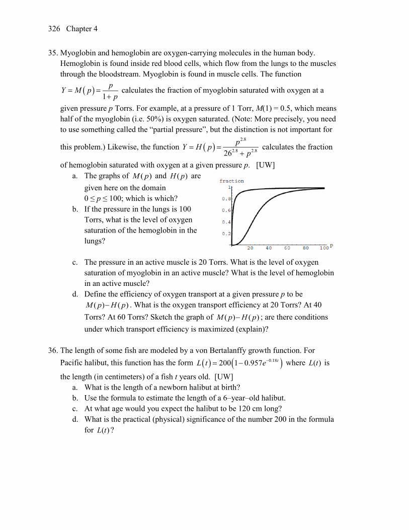
Chapter 4 326

35. Myoglobin and hemoglobin are oxygen-carrying molecules in the human body. Hemoglobin is found inside red blood cells, which flow from the lungs to the muscles through the bloodstream. Myoglobin is found in muscle cells. The function

( )1

pY M pp

= =+

calculates the fraction of myoglobin saturated with oxygen at a

given pressure p Torrs. For example, at a pressure of 1 Torr, M(1) = 0.5, which means half of the myoglobin (i.e. 50%) is oxygen saturated. (Note: More precisely, you need to use something called the “partial pressure”, but the distinction is not important for

this problem.) Likewise, the function ( )2.8

2.8 2.826pY H p

p= =

+ calculates the fraction

of hemoglobin saturated with oxygen at a given pressure p. [UW] a. The graphs of ( )M p and ( )H p are

given here on the domain 0 ≤ p ≤ 100; which is which?

b. If the pressure in the lungs is 100 Torrs, what is the level of oxygen saturation of the hemoglobin in the lungs?

c. The pressure in an active muscle is 20 Torrs. What is the level of oxygen saturation of myoglobin in an active muscle? What is the level of hemoglobin in an active muscle?

d. Define the efficiency of oxygen transport at a given pressure p to be ( ) ( )M p H p− . What is the oxygen transport efficiency at 20 Torrs? At 40

Torrs? At 60 Torrs? Sketch the graph of ( ) ( )M p H p− ; are there conditions under which transport efficiency is maximized (explain)?

36. The length of some fish are modeled by a von Bertalanffy growth function. For

Pacific halibut, this function has the form ( ) ( )0.18200 1 0.957 tL t e−= − where ( )L t is

the length (in centimeters) of a fish t years old. [UW] a. What is the length of a newborn halibut at birth? b. Use the formula to estimate the length of a 6–year–old halibut. c. At what age would you expect the halibut to be 120 cm long? d. What is the practical (physical) significance of the number 200 in the formula

for ( )L t ?


37. A cancer cell lacks normal biological growth regulation and can divide continuously. Suppose a single mouse skin cell is cancerous and its mitotic cell cycle (the time for the cell to divide once) is 20 hours. The number of cells at time t grows according to an exponential model. [UW]

a. Find a formula ( )C t for the number of cancerous skin cells after t hours. b. Assume a typical mouse skin cell is spherical of radius 50×10−4 cm. Find the

combined volume of all cancerous skin cells after t hours. When will the volume of cancerous cells be 1 cm3?

38. A ship embarked on a long voyage. At the start of the voyage, there were 500 ants in

the cargo hold of the ship. One week into the voyage, there were 800 ants. Suppose the population of ants is an exponential function of time. [UW]

a. How long did it take the population to double? b. How long did it take the population to triple? c. When were there be 10,000 ants on board? d. There also was an exponentially growing population of anteaters on board. At

the start of the voyage there were 17 anteaters, and the population of anteaters doubled every 2.8 weeks. How long into the voyage were there 200 ants per anteater?

39. The populations of termites and spiders in a certain house are growing exponentially. The house contains 100 termites the day you move in. After 4 days, the house contains 200 termites. Three days after moving in, there are two times as many termites as spiders. Eight days after moving in, there were four times as many termites as spiders. How long (in days) does it take the population of spiders to triple? [UW]

Chapter 4 328

Section 4.7 Fitting Exponential Models to Data In the previous section, we saw number lines using logarithmic scales. It is also common to see two dimensional graphs with one or both axes using a logarithmic scale. One common use of a logarithmic scale on the vertical axis is to graph quantities that are changing exponentially, since it helps reveal relative differences. This is commonly used in stock charts, since values historically have grown exponentially over time. Both stock charts below show the Dow Jones Industrial Average, from 1928 to 2010.

Both charts have a linear horizontal scale, but the first graph has a linear vertical scale, while the second has a logarithmic vertical scale. The first scale is the one we are more familiar with, and shows what appears to be a strong exponential trend, at least up until the year 2000.

Section 4.7 Fitting Exponential Models to Data 329

Example 1 There were stock market drops in 1929 and 2008. Which was larger? In the first graph, the stock market drop around 2008 looks very large, and in terms of dollar values, it was indeed a large drop. However, the second graph shows relative changes, and the drop in 2009 seems less major on this graph, and in fact the drop starting in 1929 was, percentage-wise, much more significant. Specifically, in 2008, the Dow value dropped from about 14,000 to 8,000, a drop of 6,000. This is obviously a large value drop, and amounts to about a 43% drop. In 1929, the Dow value dropped from a high of around 380 to a low of 42 by July of 1932. While value-wise this drop of 338 is much smaller than the 2008 drop, it corresponds to a 89% drop, a much larger relative drop than in 2008. The logarithmic scale shows these relative changes.

The second graph above, in which one axis uses a linear scale and the other axis uses a logarithmic scale, is an example of a semi-log graph.

Semi-log and Log-log Graphs A semi-log graph is a graph with one axis using a linear scale and one axis using a logarithmic scale. A log-log graph is a graph with both axes using logarithmic scales.

Example 2

Plot 5 points on the graph of xxf )2(3)( = on a semi-log graph with a logarithmic scale on the vertical axis. To do this, we need to find 5 points on the graph, then calculate the logarithm of the output value. Arbitrarily choosing 5 input values,

x f(x) log(f(x))

-3 83)2(3 3 =−

-0.426

-1 23)2(3 1 =−

0.176

0 3)2(3 0 = 0.477 2 12)2(3 2 = 1.079 5 96)2(3 5 = 1.982

Chapter 4 330

Plotting these values on a semi-log graph,

Notice that on this semi-log scale, values from the exponential function appear linear. We can show this behavior is expected by utilizing logarithmic properties. For the function xabxf =)( , finding log(f(x)) gives

( ) ( )xabxf log)(log = Utilizing the sum property of logs, ( ) ( ) ( )xbaxf loglog)(log += Now utilizing the exponent property, ( ) ( ) ( )bxaxf loglog)(log +=

This relationship is linear, with log(a) as the vertical intercept, and log(b) as the slope. This relationship can also be utilized in reverse. Example 3

An exponential graph is plotted on semi-log axes. Find a formula for the exponential function g(x) that generated this graph.

The graph is linear, with vertical intercept at (0, 1). Looking at the change between the

points (0, 1) and (4, 4), we can determine the slope of the line is 43 . Since the output is

log(g(x)), this leads to the equation ( ) xxg431)(log += .


We can solve this formula for g(x) by rewriting in exponential form and simplifying:

( ) xxg431)(log += Rewriting as an exponential,

xxg 4

3110)(

+= Breaking this apart using exponent rules,

xxg 4

31 1010)( ⋅= Using exponent rules to group the second factor,

x

xg

⋅= 4

31 1010)( Evaluating the powers of 10,

( )xxg 623.510)( = Try it Now 1. An exponential graph is plotted on a semi-log graph below. Find a formula for the

exponential function g(x) that generated this graph.

Fitting Exponential Functions to Data Some technology options provide dedicated functions for finding exponential functions that fit data, but many only provide functions for fitting linear functions to data. The semi-log scale provides us with a method to fit an exponential function to data by building upon the techniques we have for fitting linear functions to data.

To fit an exponential function to a set of data using linearization 1. Find the log of the data output values 2. Find the linear equation that fits the (input, log(output)) pairs. This equation will

be of the form log(f(x)) = b + mx. 3. Solve this equation for the exponential function f(x)

Chapter 4 332

Example 4 The table below shows the cost in dollars per megabyte of storage space on computer hard drives from 1980 to 2004, and the data is shown on a standard graph to the right, with the input changed to years after 1980.

This data appears to be decreasing exponentially. To find a function that models this decay, we would start by finding the log of the costs.

As hoped, the graph of the log of costs appears fairly linear, suggesting an exponential function will fit the original data will fit reasonably well. Using technology, we can find a linear equation to fit the log(Cost) values. Using t as years after 1980, linear regression gives the equation:

ttC 231.0794.2))(log( −= Solving for C(t),

ttC 231.0794.210)( −= ttC 231.0794.2 1010)( −⋅=

( )ttC 231.0794.2 1010)( −⋅= ( )ttC 5877.0622)( ⋅=

This equation suggests that the cost per megabyte for storage on computer hard drives is decreasing by about 41% each year. Using this function, we could predict the cost of storage in the future. Predicting the cost in the year 2020 (t = 40):

Year Cost per MB 1980 192.31 1984 87.86 1988 15.98 1992 4 1996 0.173 2000 0.006849 2004 0.001149

Year t Cost per MB log(Cost) 1980 0 192.31 2.284002 1984 4 87.86 1.943791 1988 8 15.98 1.203577 1992 12 4 0.60206 1996 16 0.173 -0.76195 2000 20 0.006849 -2.16437 2004 24 0.001149 -2.93952


( ) 000000364.05877.0622)40( 40 ≈=C dollars per megabyte, a really small number. That is equivalent to $0.36 per terabyte of hard drive storage. Comparing the values predicted by this model to the actual data, we see the model matches the original data in order of magnitude, but the specific values appear quite different. This is, unfortunately, the best exponential model that can fit the data. It is possible that a non-exponential model would fit the data better, or there could just be wide enough variability in the data that no relatively simple model would fit the data any better.

Try it Now 2. The table below shows the value V, in billions of dollars, of US imports from China t

years after 2000.

This data appears to be growing exponentially. Linearize this data and build a model

to predict how many billions of dollars of imports were expected in 2011.

Important Topics of this Section Semi-log graph Log-log graph Linearizing exponential functions Fitting an exponential equation to data

Try it Now Answers 1. ( )xxxg 5.025.02 101010)( =− == . xxf )3162.0(100)( = 2. ttV )2078.1(545.90)( = . Predicting in 2011, 45.722)11( =V billion dollars

Year Actual Cost per MB

Cost predicted by model

1980 192.31 622.3 1984 87.86 74.3 1988 15.98 8.9 1992 4 1.1 1996 0.173 0.13 2000 0.006849 0.015 2004 0.001149 0.0018

year 2000 2001 2002 2003 2004 2005 t 0 1 2 3 4 5 V 100 102.3 125.2 152.4 196.7 243.5

Chapter 4 334

Section 4.7 Exercises Graph each function on a semi-log scale, then find a formula for the linearized function in the form ( )( )log f x mx b= + .

1. ( ) ( )4 1.3 xf x = 2. ( ) ( )2 1.5 xf x =

3. ( ) ( )10 0.2 xf x = 4. ( ) ( )30 0.7 xf x = The graph below is on a semi-log scale, as indicated. Find a formula for the exponential function

( )y x .

5. 6.

7. 8.


Use regression to find an exponential function that best fits the data given. 9. x 1 2 3 4 5 6

y 1125 1495 2310 3294 4650 6361

10. x 1 2 3 4 5 6 y 643 829 920 1073 1330 1631

11. x 1 2 3 4 5 6 y 555 383 307 210 158 122

12. x 1 2 3 4 5 6 y 699 701 695 668 683 712

13. Total expenditures (in billions of dollars) in the US for nursing home care are shown below.

Use regression to find an exponential function that models the data. What does the model predict expenditures will be in 2015?

Year 1990 1995 2000 2003 2005 2008 Expenditure 53 74 95 110 121 138

14. Light intensity as it passes through water decreases exponentially with depth. The data

below shows the light intensity (in lumens) at various depths. Use regression to find an function that models the data. What does the model predict the intensity will be at 25 feet?

Depth (ft) 3 6 9 12 15 18 Lumen 11.5 8.6 6.7 5.2 3.8 2.9

15. The average price of electricity (in cents per kilowatt hour) from 1990 through 2008 is given

below. Determine if a linear or exponential model better fits the data, and use the better model to predict the price of electricity in 2014.

Year 1990 1992 1994 1996 1998 2000 2002 2004 2006 2008 Cost 7.83 8.21 8.38 8.36 8.26 8.24 8.44 8.95 10.40 11.26

16. The average cost of a loaf of white bread from 1986 through 2008 is given below. Determine

if a linear or exponential model better fits the data, and use the better model to predict the price of a loaf of bread in 2016.

Year 1986 1988 1990 1995 1997 2000 2002 2004 2006 2008 Cost 0.57 0.66 0.70 0.84 0.88 0.99 1.03 0.97 1.14 1.42

Chapter 4 336

Chapter 4: Exponential and Logarithmic Functions 4.pdf · Write an exponential function for...

Documents

Transcript of Chapter 4: Exponential and Logarithmic Functions 4.pdf · Write an exponential function for...