Chapter 4: Elliptic Generation Systems - Freeebrary.free.fr/Mesh Generation/Handbook_of_Grid_...

4Elliptic Generation

Systems

4.1 Introduction4.2 Two-Dimensional Grid Generation

Harmonic Maps, Grid Control Maps, and Poisson Systems • Discretization and Solution Method • Construction of Grid Control Maps • Best Practices

4.3 Surface Grid Generation 4.4 Volume Grid Generation 4.5 Research Issues and Summary 4.6 Further Information

4.1 Introduction

Since the pioneering work of Thompson on elliptic grid generation, it is known that systems of ellipticsecond-order partial differential equations produce the best possible grids in the sense of smoothnessand grid point distribution. The grid generation systems of elliptic quasi-linear second-order partialdifferential equations are so-called Poisson systems with control functions to be specified. The secret ofeach “good” elliptic grid is the method to compute the control functions [3].

Originally Thompson and Warsi introduced the Poisson systems by considering a curvilinear coordi-nate system that satisfies a system of Laplace equations and is transformed to another coordinate system[30,35]. Then this new coordinate system satisfies a system of Poisson equations with control functionscompletely specified by the transformation between the two coordinate systems. However, Thompsondid not advocate to use this approach for grid generation. Instead he proposed to use the Poisson systemwith control functions specified directly rather than through a transformation [30]. Since then, the generalapproach is to compute the control functions at the boundary and to interpolate them from the bound-aries into the field [5,29]. The standard approach used to achieve grid orthogonality and specified cellheight on boundaries has been the iterative adjustment of the control functions in the Poisson systems(Chapter 6), first introduced by Sorenson of NASA Ames in the GRAPE code in the 1980s [24]. Variousmodifications of this basic concept have been introduced in several codes, and the general approach isnow common [23,5,29]. Although successful, it appears that the method is not easy to apply in practice[14]. Even today, new modifications are proposed to improve the grid quality and to overcome numericaldifficulties in solving the Poisson grid generation equations [23,16,12].

In this chapter we describe a useful alternative approach to specify the control functions. It is basedon Thompson’s and Warsi’s original idea to define the control functions by a transformation. Thetransformation, which we call a grid control map, is a differentiable one-to-one mapping from compu-tational space to parameter space. The independent variables of the parameter space are harmonicfunctions in physical space. The map from physical space to parameter space is called the harmonic map

Stefan P. Spekreijse

©1999 CRC Press LLC

(Chapter 8). The composition of the grid control map and the inverse of the harmonic map obeys thefamiliar Poisson systems with control functions completely defined by the grid control map. The con-


struction of appropriate grid control maps such that the corresponding grid in physical space has desiredproperties is the main issue of this chapter.

One of the main advantages of this approach is that the method is noniterative. If an appropriate gridcontrol map has been constructed, then the corresponding grid control functions of the Poisson system arecomputed and their values remain unchanged during the solution of the Poisson system. Picard iterationappears to be a simple and robust method to solve the Poisson system with fixed control functions.

Another advantage is that the construction of an appropriate grid control map can be considered asa numerical implementation of the constructive proof for the existence of the desired grid in physicalspace. If the grid control map is one-to-one, then the composition of the grid control map and the inverseof the harmonic maps exist so that the solution of the Poisson system is well-defined.

This chapter is organized as follows. Section 4.2 concerns the two-dimensional case. Although pub-lished earlier [25], the 2D Poisson system together with the expressions to compute the control functionsfrom the grid control map are given for completeness. The solution of the Poisson system by Picarditeration is shortly described. Section 4.2.3 describes methods to construct appropriate grid control maps.Boundary orthogonality is obtained by applying Dirichlet–Neumann boundary conditions for the har-monic map and by applying cubic Hermite interpolation in parameter space. In that case, the harmonicmap is quasi-conformal. This observation leads to the construction of appropriate grid control maps suchthat the solution of the Poisson system generates an orthogonal grid in physical space with boundary gridpoints fixed on two adjacent edges but moved along the other two opposite edges (see Chapter 7). Thisresult is similar to that reported by Kang and Leal [13], although they used the Ryskin–Leal grid generationequations [19] instead of the Poisson grid generation equations. Section 4.2.4 shows generated grids inphysical space for well-defined geometries so that the reader is able to recompute the grids (by themethods presented in this chapter or by his/her own favorite methods for comparison). The correspond-ing constructed grid control maps are shown as grids in parameter space.

Section 4.3 briefly describes how the same methods to construct appropriate grid control maps for2D grids can also be used for grid generation on surfaces in 3D physical space (see Chapter 9). It is shownthat surface grid generation on minimal surfaces (soap films) is in fact the same as 2D grid generation.Conceptually, the same methods can also be used for parametrically defined surfaces, although thenumerical implementation is completely different.

The extension to volume grid generation is described in Section 4.4. The construction of appropriategrid control maps for 3D domains is less well developed than for 2D domains. However, a method toconstruct a grid control map has been proposed which works surprisingly well for many applications.

The now-standard procedure in multi-block structured grid generation codes is to first generate surfacegrids on block faces, both boundary and interior block interfaces, from grid point distributions placedon the face edges by distribution functions. Then volume grids are generated within the blocks. For thisreason, the elliptic grid generation methods described in this chapter assume fixed position of theprescribed boundary grid points.

4.2 Two-Dimensional Grid Generation

4.2.1 Harmonic Maps, Grid Control Maps and Poisson SystemsConsider a simply connected bounded domain D in two-dimensional space with Cartesian coordinates

(x, y)T. Suppose that D is bounded by four edges E1, E2, E3, E4. Let (E1, E2) and let (E3, E4) be the twopairs of opposite edges as shown in Figure 4.1.

A harmonic map is defined as a differentiable one-to-one map from D onto a unit square such that

1. The boundary of D is mapped onto the boundary of the unit square,2. The vertices of D are mapped, in the proper sequence, onto the corners of the unit square,3. The two components of the map are harmonic functions in the interior of D.

rx


Let : D a P be a harmonic map where the parameter space P is the unit square in a two-dimensionalspace with Cartesian coordinates = (s, t)T. Assume that

• at edge E1 and at edge E2,

• at edge E3 and at edge E4.

The problem of generating an appropriate grid in the physical domain D can be effectively reducedto a simpler problem of generating an appropriate grid in the parameter space P, which can after that bemapped into D, by using the inverse of the harmonic map : P a D.

Define the computational space C as the unit square in a two-dimensional space with Cartesiancoordinates . A grid control map : C a P is defined as a differentiable one-to-one map fromC onto P and maps a uniform grid in C to a nonuniform (in general) grid in P. Assume that

• and ,

• and .

Then the computational coordinates also fulfill



The composition of a grid control map : C a P and the inverse of the harmonic map : P a Ddefine a map : C a D which transforms a uniform grid in C to a nonuniform (in general) grid in D.The composite map obeys a quasi-linear system of elliptic partial differential equations, known as thePoisson grid generation equations, with control functions completely defined by the grid control map. Thesecret of each “good” elliptic grid generation method is the method of computing appropriate controlfunctions, which is thus equivalent to constructing appropriate grid control maps.

We will now derive the quasi-linear system of elliptic partial differential equations which the compositemapping = ( (ξ)) has to fulfill. Suppose that the harmonic map and the grid control map are definedso that the composite map exists. Introduce the two covariant base vectors (see Chapter 2)

(4.1)

and define the covariant metric tensor components as the inner product of the covariant base vectors

(4.2)

The two contravariant base vectors 1 = ∇ ξ = (ξx, ξy)T and 2 = ∇ η = (ηx, ηy)T obey

(4.3)

FIGURE 4.1 Composite map from computational (ξ,η) space to a domain D in Cartesian (x,y) space.

rs

rs

s 0≡ s 1≡t 0≡ t 1≡

rx

rξ x h,( )T=

rs

s 0 h,( ) 0≡ s 1 h,( ) 1≡t x 0,( ) 0≡ t x 1,( ) 1≡

x 0≡ x 1≡h 0≡ h 1≡

rs

rx

rx

rx

rx

rs

rr

r rr

ra

xx a

xx1 2= ∂

∂= = ∂

∂=

ξ ηξ η,

r r ra a a i ji j i j, , { , } { , }= ( ) = = 1 2 1 2

ra

ra

r ra a i ji

j ji,( )δ = { , } = { , }1 2 1 2

with

δ

ji

the Kronecker symbol. Define the contravariant metric tensor components

r r


(4.4)

so that

(4.5)

and

(4.6)

Introduce the determinant J2 of the covariant metric tensor: J 2 = a11a22 – a212 .

Now consider an arbitrary function φ = φ (ξ, η). Then φ is also defined in domain D, and the Laplacianof φ is expressed as

(4.7)

which may be found in Chapter 2 and in every textbook on tensor analysis and differential geometry(for example, see [15]). Take as special cases respectively and . Then Eq. 4.7 yields

(4.8)

Thus the Laplacian of φ can also be expressed as

(4.9)

Substitution of respectively and in this equation yields

(4.10)

(4.11)

Using these equations and the property that s and t are harmonic in domain D, thus ∆s = 0 and∆t = 0, we find the following expressions for the Laplacian of ξ and η:

(4.12)

where

(4.13)

a a a i jij i j= ( ) = =, { , } { , } 1 2 1 2

a a

a a

a a

a a

11 12

12 22

11 12

12 22

1

0

0

1

=

r r r r r r

r r r r r ra a a a a a a a a a

a a a a a a a a a a

1 111

122

121

222

1 111

122

2 121

222

= + = +

= + = +

2

∆φ φ φ φ φ φ φξ η ξ ξ η η= + − +( ) + +( )xx yy J

Ja Ja Ja Ja1 11 12 12 22{ }

f x≡ f h≡

∆ ∆ξ ηξ η ξ η

= ( ) + ( ) = ( ) + ( )1 111 12 12 22

JJa Ja

JJa Ja{ } { }

∆ ∆ ∆φ φ φ φ ξφ ηφξξ ξη ηη ξ η= + + + +a a a11 12 222

f s≡ f t≡

∆ ∆ ∆s a s a s a s s s= + + + +11 12 222ξξ ξη ηη ξ ηξ η

∆ ∆ ∆t a t a t a t t t= + + + +11 12 222ξξ ξη ηη ξ ηξ η

∆∆

ξη

= + +a P a P a P1111

1212

22222

r r r

r r rP T

s

tP T

s

tP T

s

t111

121

221= −

= −

= −

− − −ξξ

ξξ

ξη

ξη

ηη

ηη

and the matrix T is defined as


(4.14)

The six coefficients of the vectors 11 = (P111 , P2

11 ) T, 12 = (P112 , P2

12 ) T and 22 = (P122 , P2

22 ) T are the so-called control functions. The six control functions are completely defined and easily computed for a givengrid control map = ( ). Different and less useful expressions of these control functions can also befound in [30,35].

Finally, substitution of φ ≡ in Eq. 4.9 yields

(4.15)

Substituting Eq. 4.12 into this equation and using the fact that ∆ ≡ 0, we arrive at the familiar Poissongrid generation system:

(4.16)

Using Eqs. 4.2, and 4.5 we find the following well-known expressions for the contravariant metrictensor components:

(4.17)

Thus the Poisson grid generation system defined by Eq. 4.16 can be simplified by multiplication with J2.Then we obtain:

(4.18)

This equation, together with the expressions for the control functions Pkij given by Eq. 4.13, is the two-

dimensional grid generation system. For a given grid control map, so that the six control functions inEq. 4.18 are given functions of ξ and η, boundary conforming grids in the interior of domain D arecomputed by solving this quasi-linear system of elliptic partial differential equations with prescribedboundary grid points as Dirichlet boundary conditions. The discretization and solution method of thisPoisson system is discussed in the next section. The construction of appropriate grid control maps suchthat the corresponding grid in physical space has desired properties is discussed in the remaining sections.

4.2.2 Discretization and Solution Method

Consider a uniform rectangular grid of (N + 1) × (M + 1) points in computational space C defined as

(4.19)

Assume that i, j is prescribed on the boundary of this grid and consider the computation of i, j in theinterior of the computational grid based on the solution of the Poisson system defined by Eq. 4.18.

Ts s

t t=

ξ η

ξ η

rP

rP

rP

rs

rs

rξ

rx

∆ ∆ ∆

r r r r r rx a x a x a x x x= + + + +11 12 222ξξ ξη ηη ξ ηξ η

rx

a x a x a x a P a P a P x

a P a P a P x

11 12 22 11111 12

121 22

221

11112 12

122 22

222

2 2

2 0

r r r r

rξξ ξη ηη ξ

η

+ + + + +( )+ + +( ) =

J a a x x J a a x x J a a x x2 11

222 12

122 22

11= = ( ) = − = −( ) = = ( )r r r r r rη η ξ η ξ ξ, , ,

a x a x a x a P a P a P x

a P a P a P x

22 12 11 22 111

12 121

11 221

22 112

12 122

11 222

2 2

2 0

r r r r

rξξ ξη ηη ξ

η

− + + − +( )+ − +( ) =

ξ ξ η ηij i i j ji N j M i N j M= = = = = =/ /, ... ... 0 0

rx

rx


Assume that a grid control map : C a P has been constructed. Thus the values sij and tij are knownat each grid point. At each interior grid point (i, j) ∈ (1… N – 1, 1… M – 1), the six control functionsP1

ll, P2l1, P1

12, P212, P1

22, P222 defined by Eq. 4.13 are now easily computed using central differences for the

discretization of sξξ , sξη , sηη , sξ , sη and tξξ , tξη , tηη , tξ , tη.The iterative solution process of the nonlinear elliptic Poisson grid generation system defined by

Eq. 4.18 can be simply obtained by Picard iteration. Rewrite the Poisson system as

(4.20)

with

(4.21)

The iterative solution by Picard iteration can be written as

(4.22)

where k is the Picard index and

(4.23)

Thus, a current approximate solution

(4.24)

FIGURE 4.2 Boundary conditions for both control of orthogonality and first grid cell height.

rs

Px Qx Rx Sx Txr r r r rξξ ξη ηη ξ η− + + + =2 0

P x x Q x x R x x

S PP QP RP

T PP QP RP

= ( ) = ( ) = ( )= − +

= − +

r r r r r rη η ξ η ξ ξ. . .

111

121

221

112

122

222

2

2

P x Q x R x S x T xk k k k k k k k k k− − − − −− + + + =1 1 1 1 12 0

r r r r rξξ ξη ηη ξ η

P x x Q x x R x x

S P P Q P R P

T P P Q P R

k k k k k k k k k

k k k k

k k k k

− − − − − − − − −

− − − −

− − − −

= ( ) = ( ) ≈ ( )= − +

= − +

1 1 1 1 1 1 1 1 1

1 1111 1

121 1

221

1 1112 1

122

2

2

r r r r r rη η ξ η ξ ξ, , ,

11222P

r rx x i N j Mk

ijk− −= = =1 1 0 0{ }, ... , ...


is improved by the following steps:

• Compute at interior grid points the coefficients Pk-1,Qk–1,Rk-1,Sk-1,Tk-1 by applying central differ-ences for the discretization of and . Note that the six control functions remain unchangedduring the iterative procedure.

• Discretize at interior grid points , , , , using central differences.

• After the discretization of , , , , we arrive at a linear system of equations for theunknowns i = 1… N – 1, j = … M – 1. At each interior grid point we have a nine-point stencil.Boundary grid points are prescribed and remain unchanged. This linear system can be solved bya black-box multigrid solver. Such a multigrid solver is called twice to compute the two componentsx k

ij and ykij of . The solution of the linear system provides a better approximate solution .

The following algorithm describes the computation of an interior grid in domain D with prescribedboundary grid points and a given grid control map.

Algorithm 1. Grid Generation.

1. Compute the six control functions from the grid control map.2. Compute an initial grid in the interior of domain D by a simple algebraic grid generation method

(see Chapter 3). The quality of the initial grid is unimportant, and severe grid folding is allowed.The initial grid is used as starting solution for the Picard iteration process. The final grid will beindependent of the initial grid.

3. Solve the quasi-linear Poisson grid generation equations iteratively by Picard iteration. The fixedposition of the boundary grid points define Dirichlet boundary conditions. In general, a sufficientlyconverged grid is obtained in about 10 Picard iterations. The residual is then typically decreasedby a factor 1000.

4.2.3 Construction of Grid Control Maps

4.2.3.1 Laplace Grids

The simplest grid control map is the identity map = . The six control functions are identical zero andthe Poisson grid generation system defined by Eq. 4.18 simplifies to a22 ξξ – 2a12 ξη + a11 ηη = 0, whichis equivalent with ∆ξ = 0 and ∆η = 0, according to Eq. 4.12.

Grids based on this equation are the so-called Laplace (or Harmonic) grids, which were first introducedby Winslow [34]. The inherent smoothness of the Laplace operator makes the grid evenly spaced in theinterior. Therefore, the quality of a Laplace grid will be acceptable only as long as the boundary gridpoints are evenly spaced along the edges.

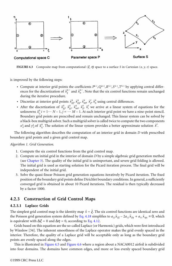
This is illustrated in Figure 4.5 and Figure 4.6 where a region about a NACA0012 airfoil is subdividedinto four domains. The domains have common edges, and more or less evenly spaced boundary grid

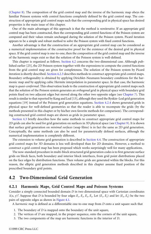
FIGURE 4.3 Composite map from computational (ξ, η) space to a surface S in Cartesian (x, y, z) space.

rxk

ξ−1 r

xkη

−1

rxk

ξξrxk

ξηrxk

ηηrxk

ξrxk

ηrxk

ξξrxk

ξηrxk

ηηrxk

ξrxk

ηrxij

k

rxij

k rxk

rs

rξ r

xrx

rx


points are prescribed. Figure 4.6 shows Laplace grids in each domain. The result is not bad for this O-type Euler mesh. (Only smooth grids are required for the solution of the Euler equations for nonviscousflow, where strong gradients near boundaries do not occur.) Laplace grids provide no control about theangle distribution between internal grid lines and the boundary. This causes slope discontinuity of thegrid lines across internal domain boundaries, as shown in Figure 4.6.

The situation is completely different for Navier–Stokes type of meshes where the grid must contain aboundary layer grid. Highly stretched grids are required for solutions of the Navier–Stokes equations forviscous flow, where large gradients occur near boundaries. Figure 4.9 shows a region about a RAE2822airfoil also subdivided into four domains. The boundary grid point distribution is highly dense near theleading and trailing edge of the airfoil. Figure 4.10 shows the Laplace grids in the four domains. Thesegrids are unacceptable because the inherent smoothness of the Laplace operator causes evenly spacedgrids so that the interior grid contains no boundary layer at all. Therefore, Laplace grids are in generalunusable in most practice.

FIGURE 4.4 Composite mapping from computational (ξ, η, ζ ) space to a domain D in Cartesian (x, y, z) space.

FIGURE 4.5 Domain boundaries near NACA0012 airfoil. The location of grid points on the domain boundariesis prescribed and fixed.


4.2.3.2 Arc Length Based Grids

Consider domain D as shown in Figure 4.1. Assume that the boundary grid points are prescribed at thefour edges of D. A boundary-conforming grid in the interior of domain D with an interior grid pointdistribution which is a good reflection of the prescribed boundary grid point distribution can be obtainedby constructing a grid control map based on normalized arc length. In order to construct such a gridcontrol, we define


• s is the normalized arc length along edges E3 and E4,


• t is the normalized arc length along edges E1 and E2.

For example, this means that along edge E3 we define s(u) = where a

is a parametrization of edge E3 in the right direction. Thus : ∂D a∂P is defined by these

requirements. The two Laplace equations ∆s = 0 and ∆t = 0, together with the above-specified Dirichlet

boundary conditions, define the harmonic map : D a P. Note that this map depends only on the shapeof domain D and is independent of the prescribed boundary grid point distribution.

The boundary grid points are prescribed at the four edges of D. Thus : ∂C a ∂D is prescribed.Because : ∂C a ∂D is prescribed and : ∂D a∂P is defined as described above, it follows that : ∂C a∂Pis also defined.

From the preceding requirements it follows that

(4.25)

where the functions saE3

, s aE4

are monotonically increasing, and

(4.26)

FIGURE 4.6 Laplace grid. Grid control map is the identity map.

s 0≡ s 1≡

t 0≡ t 1≡

r rx du x duu

o

u

u∫ ∫0

1 rx: u 0 1,[ ]Œ

x y,( ) R2Œrs

rs

rx

rx

rs

rs

s s s s s sEa

Ea0 0 1 1 0 1

3 4, , , ,η η ξ ξ ξ ξ( ) = ( ) = ( ) = ( ) ( ) = ( )

t t t t t tEa

Eaξ ξ η η η η, , , ,0 0 1 1 0 1

1 2( ) = ( ) = ( ) = ( ) ( ) = ( )

where the functions taEl, ta

E2are also monotonically increasing. The superscript a is used to indicate that

these functions measure the normalized arc length at the boundary grid points.r


The grid control map : C a P is now defined by the following two algebraic equations:

(4.27)

(4.28)

Eq. 4.27 implies that a coordinate line ξ = const. is mapped to the parameter space P as a straight line:s is a linear function of t, and Eq. 4.28 implies that a grid line η = const. is also mapped to P as a straightline: t is a linear function of s. For given values of ξ and η, the corresponding s and t values are foundas the intersection point of the two straight lines. It can be easily verified that the grid control map is adifferentiable and one-to-one because of the positiveness of the Jacobian: sξ tη – sηtξ > 0.

The discrete computation of the grid control map is straightforward. For a grid of (N + 1) × (M + 1)points, the distance between succeeding grid points at the boundary are computed as

(4.29)

(4.30)

Define the length of edges E1, E2 E3, E4 by

(4.31)

and the normalized distances as

(4.32)

(4.33)

The discrete components si,j and ti,j of the grid control map are computed at the boundary by

(4.34)

(4.35)

and

(4.36)

(4.37)

The interior values are defined according to Eq. 4.27 and Eq. 4.28 and are thus found by solvingsimultaneously the two linear algebraic equations,

s

s s t s tEa

Ea= ( ) −( ) + ( )

3 41ξ ξ

t t s t sEa

Ea= ( ) −( ) + ( )

1 21η η

d x x d x x j Mj j j N j N j N j, , , , , ,0 0 0 1 1 1= − = −− −

r r r r = ...

d x x d x x i Ni i i i M i M i M, , , , , , ,0 0 1 0 1 1= − = −− −r r r r

= ...

L d L d L d L dE jj

M

E N jj

M

E ii

N

E i Mi

N

1 2 3 401 1

01 1

= = = == = = =∑ ∑ ∑ ∑, , , ,

d d L d d L j Mo j o j E N j N j E, , , ,/ / ...= = =1 2

1

d d L d d L i Ni i E i M i M E, , , ,/ / ...0 0 3 41= = =

s s j Mo j N j, , ...= = =0 1 0

t t i Ni i M, , ...0 0 1 0= = =

s s d s s d i Ni i i i M i M i M, , , , , ,0 1 0 0 1 1= + = +− − = ...

t t d t t d j Mo j j N j i M N j N j, , , , , ,= + = +− −0 1 1 1 = ...


(4.38)

(4.39)

for each pair (i, j) ∈ (1…N – 1, 1…M – 1).The next algorithm summarizes the computation of arc length-based grid in the interior of D.

Algorithm 2. Arc length-based grids

1. Compute the four edge functions taEl, ta

E2, sa

E3and sa

E4from the boundary grid point distribution.

2. Compute the grid control map according to Eq. 4.27 and Eq. 4.28.3. Compute the corresponding interior grid in D as described in Algorithm 1.

Illustrations of boundary conforming grids obtained with this grid control map are shown in Figure 4.7and Figure 4.11. As opposed to Laplace grids, the interior grid point distribution is always a goodreflection of the prescribed boundary grid point distribution. Grid folding hardly ever occurs, becauseboth the grid control map and the harmonic map are one-to-one. When grid folding occurs, then itmust be caused by discretization errors [18]. Hence, grid folding will always disappear when the grid issufficiently refined.

A shortcoming of this grid control map is that there is no control about the angle distribution betweeninterior grid lines and the boundary edges of the domain. It is often desired that the interior grid linesare orthogonal at the boundary edges. For example, viscous flow simulations often require orthogonalityof the grid in a boundary layer. This can be achieved with a grid control map as constructed below.

4.2.3.3 Grid Orthogonality at the Boundary

Consider domain D with prescribed boundary grid points. Suppose that it is desired to generate aboundary-conforming grid in the interior of D which is orthogonal at all four edges of domain D. Thiscan be achieved by imposing Dirichlet–Neumann boundary conditions for the harmonic map:

FIGURE 4.7 Arc length-based grid.

s s t s ti j i i j i M i j, , , , ,= −( ) +0 1

t t s t si j j i j N j i j, , , , ,= −( ) +0 1


• along edges E3 and E4, where n is the outward normal direction,

s 0≡ s 1≡∂s ∂n⁄



• along edges E1 and E2, where n is the outward normal direction.

The two Laplace equations ∆s = 0 and ∆t = 0, together with the above specified boundary conditions,define the harmonic map : D a P. Again this map depends only on the shape of domain D and isindependent of the prescribed boundary grid point distribution.

The Neumann boundary conditions ∂s/∂n = 0 along edges E3 and E4 imply that a parameter line s =const. in P will be mapped into domain D by the inverse of the harmonic map as a curve which isorthogonal at those edges. Similarly, a parameter line t = const. in P will be mapped as a curve in Dwhich is orthogonal at edge E1 and edge E2. These properties can be used to construct a grid control mapsuch that the interior grid in D will be orthogonal at the boundary.

The boundary grid points are prescribed at the four edges of D. Thus : ∂C a ∂D is prescribed.Because : ∂C a ∂D is prescribed and : ∂D a ∂P is also defined, it follows that : ∂C a ∂P is also defined.

From the preceding requirements it follows that

(4.40)

where the functions s0E3

, s0E4

are monotonically increasing, and

(4.41)

where the functions t0E1

, t0E2

are also monotonically increasing. The superscript 0 is used to indicate thatthese functions are constructed in a way to obtain grid orthogonality at the boundary.

The grid control map : C a P is now defined by

(4.42)

(4.43)

where H0 and H1 are cubic Hermite interpolation functions defined as

(4.44)

Note that H0 (0) = 1, H0′ (0) = 0, H0 (1) = 0, H0

′(1) = 0 and H1(0) = 0, H ′1 (0) = 0, H1(1) = 1, H ′

1 (1) =0. It follows from Eq. 4.42 that a coordinate line ξ = const. in C is mapped to parameter space P as acubic curve (with t as dependent variable) which is orthogonal at both edge E3 and edge E4 in P. Such acurve in parameter space P will thus be mapped by the inverse of the harmonic map : P a D as a curvewhich is orthogonal at both edge E3 and edge E4 in D. Similar observations can be made for coordinatelines η = const. Thus the grid will be orthogonal at all four edges in domain D.

Grid orthogonality at boundaries may introduce grid folding. Fortunately, grid folding will not easilyarise. From Eq. 4.42 it follows that two different coordinate lines ξ = ξ1, ξ = ξ2, ξ1 ≠ ξ2 are mapped toparameter space P as two disjunct cubic curves which are orthogonal at both edge E3 and edge E4 in P.This is due to the fact that s0

E3(ξ) and s0

E4(ξ) are monotonically increasing functions. The same holds for

different coordinate lines η = η1, η = η2, η1≠ η2. For given values of ξ and η, the corresponding s andt values are found as intersection point of two cubic curves. However, such two cubic curves may have

t 0≡ t 1≡∂t ∂n⁄

rs

rx

rx

rs

rs

s s s s s sE E0 0 1 1 0 13 4

0 0, , , ,η η ξ ξ ξ ξ( ) = ( ) = ( ) = ( ) ( ) = ( )

t t t t tE Eξ ξ η η η η, , , ,0 0 1 1 0 11 2

0 0( ) = ( ) = ( ) = ( ) ( ) = ( ) t

rs

s s H t s H tE E= ( ) ( ) + ( ) ( )3 4

00

01ξ ξ

t t H s t H sE E= ( ) ( ) + ( ) ( )1 2

00

01η η

H s s s H s s s02

121 2 1 3 2( ) = +( ) −( ) ( ) = −( ) ≤ ≤ 0 s 1

rx

more than one intersection point. In that case, grid folding will occur. However, in practice we hardlyever encounter grid folding due to orthogonalization of the grid at the boundary.


We have described a method to obtain an orthogonal grid at all four edges of domain D. In practice,orthogonality of the grid is often only desired at less than four edges. Suppose for example that it is onlydesired to have an orthogonal grid at edge E3. Then take tE1

(η) = t0E1(η), tE2

(η) = t0E2

(η), sE4(ξ) = s0

E4(ξ)

and sE3(ξ) = s0E3

(ξ). Furthermore, the grid control map : C a P is such that a coordinate line η = const.is mapped to P as a straight line and a coordinate line ξ = const. is mapped to P as a parabolic curve(with t as dependent variable) which is only orthogonal at edge E3 in P. For given values of ξ and η, thecorresponding s and t values are then found as intersection point of a straight line and a parabolic curve.

The discrete computation of the grid control map is more complicated when grid orthogonality isrequired. We have seen that for a grid control map based on normalized arc length, thefunctions t0El

, t0E2

, s0E3

and s0E4

can be directly computed from the prescribed boundary grid points only.However, when grid orthogonality is required, the functions t0

E1, t0

E2, s0

E3 and s0

E4 can only be found by

solving the Laplace equations ∆s = 0 and ∆t = 0 supplied with the above mentioned Dirichlet–Neumannboundary conditions. The solution of the Laplace equations ∆s = 0 and ∆t = 0 supplied with the boundaryconditions requires an initial folding-free grid in the interior of domain D. Therefore, an orthogonal gridat the boundary is in general obtained in three steps:

Algorithm 3. Grid orthogonality at boundary

1. Compute an initial boundary conforming grid in the interior of D without grid folding. Such agrid can be computed using the grid control map based on normalized arc length as described inAlgorithm 2.

2. Solve on this mesh ∆s = 0 and ∆t = 0 supplied with the above specified Dirichlet–Neumannboundary conditions. A solution method is described in [19]. The solution at the boundary definesthe edge functions t0

E1, t 0E2

, s 0E3 and s 0

E4.

3. Compute the grid control map according to Eq. 4.42 and Eq. 4.43.4. Compute the corresponding interior grid in D as described in Algorithm 1.

Illustrations of boundary conforming grids obtained with this grid control map are shown in Figure 4.8and Figure 4.19. The common interior boundary edges of the four domains can hardly be recognizedany more because of the excellent grid orthogonality at these edges. The grid spacing of the interior gridis also good in both cases. For more information on grid orthogonality at the boundary, see Chapter 6.

In the next section we will prove that the harmonic map : D a P supplied with Dirichlet–Neumannboundary conditions is quasi-conformal. This observation leads to the construction of appropriate gridcontrol maps such that the corresponding grid is orthogonal, not only at the boundary but also in theinterior of D.

4.2.3.4 Orthogonal Grids

There is a famous theorem in conformal mapping theory which states that each simply connected domainD can be mapped conformally to a rectangle R in such a way that the vertices of domain D are mapped,in the proper sequence, onto the corners of the rectangle [8,11]. The ratio of the length of two adjacentsides of the rectangle is called the conformal module M, which is a characteristic and fundamentalproperty of each domain.

Let : D a R be the conformal map where R is the rectangle [0, 1] × [0, M] in a two-dimensionalspace with Cartesian coordinates = (u, v)T. The components of the conformal map obey theCauchy–Riemann relations:

(4.45)

rs

rs

ru

ru

u

u

v

v

x

y

y

x

=−


Hence ∆u = 0 and ∆v = 0 in the interior of domain D. Furthermore, we may assume that the map :D a R obeys



From these boundary conditions and using the Cauchy–Riemann relations we can also conclude that

• ∂u/∂n = 0 along edges E3 and E4, where n is the outward normal direction,

• ∂v/∂n = 0 along edges E1 and E2, where n is the outward normal direction.

Thus the conformal map : D a R is harmonic and obeys the same set of Dirichlet–Neumann boundaryconditions as the harmonic map : D a P. Therefore the two maps are related to each other according to

(4.46)

This means that the harmonic map is quasi-conformal and obeys

(4.47)

Thus the two contravariant vectors are orthogonal but have different lengths. It is not difficult to show,using the relations between covariant and contravariant vectors given by Eq. 4.6, that the covariant vectorsfulfill

(4.48)

FIGURE 4.8 Grid with boundary orthogonality. Boundary orthogonality makes the grid smooth across internaldomain boundaries.

ru

u 0≡ u 1≡v 0≡ v M≡

ru

rs

s u tv

M= =

s

sM

t

t

x

y

y

x

=−

x

y M

y

xs

s

t

t

=−

1


so that the inverse mapping obeys

(4.49)

which is the well-known partial differential equation for quasi-conformal maps [14, page 96]. It can alsobe easily verified that the conformal module can be computed from

(4.50)

where n is the outward normal direction and σ a line element along edge E2 in D [11]. Conformal maps are angle preserving. The inverse of the conformal map : D a R is also conformal

and maps an orthogonal grid in the rectangle R to an orthogonal grid in D. Therefore, an algorithm tocompute an orthogonal grid in the interior of D with a prescribed boundary grid point distribution atall four edges may consist of the following steps:

1. Compute an initial boundary conforming grid in the interior of D without grid folding. This canbe achieved using the grid control map based on normalized arc length.

2. Solve on this mesh ∆s = 0 and ∆t = 0 supplied with Dirichlet–Neumann boundary conditions.Compute the edge functions t0

E1, t0

E2, s0

E3, and s0

E4and the conformal module M according to

Eq. 4.50.3. Map the edge functions in P to the rectangle R, using Eq. 4.46, and compute an orthogonal

boundary conforming grid in R.4. Map the orthogonal grid in R to P, again using Eq. 4.46. This grid in P defines a grid control map

that will create an orthogonal grid in the interior of D.

Thus, a difficult problem of generating an orthogonal grid in a domain D can be effectively reducedto a simpler problem of generating an orthogonal grid in the rectangle R. Unfortunately, there is nosimple algorithm available to generate an orthogonal grid in the interior of a rectangle

FIGURE 4.9 Region about RAE2822 airfoil subdivided into four domains.

M x xss tt2 0r r

+ =

Ms

ndE= ∂

∂∫ 2σ

ru


with prescribed boundary grid points at all four sides. The question of an existence proof for this problemstill remains unanswered [17]. Numerical experiments indicate that even for a rectangle it is probablynot possible to generate an orthogonal grid for all kinds of boundary grid point distributions [9].

However, if the boundary grid points have fixed positions on two adjacent edges of domain D but areallowed to move along the boundary of the other two edges, then a simple algorithm does exist to generatean orthogonal grid in D. This result is similar to that reported by Kang and Leal [13], although they usedthe Ryskin–Leal grid generation equations [19] instead of the Poisson grid generation equations. Forexample, suppose that the boundary grid points are fixed at edges E1 and E3 and are allowed to movealong edges E2 and E4. Then the algorithm becomes the following.

Algorithm 4. Grid orthogonality

1. Compute an initial boundary conforming grid in the interior of D without grid folding. Such agrid can be computed using the grid control map based on normalized arc length as described inAlgorithm 2.

2. Solve on this mesh ∆s = 0 and ∆t = 0 supplied with Dirichlet–Neumann boundary conditionsand compute the edge functions t0

E1, t 0

E2, s 0

E3, and s 0

E4.

3. The initial position of the boundary grid points at edge E2 corresponds with the edge functiont0

E2. Move the boundary grid points along edge E2 in such a way that the new position corresponds

with t0E1

. This is simply a matter of interpolation. The points along edge E4 should be moved suchthat their new position corresponds with s0

E3.

4. Define the grid control map as s(ξ,η) = s0E3

(ξ) and t(ξ,η) = t0E1

(η).5. Compute the corresponding orthogonal grid in D as described in Algorithm 1.

The grid in parameter space P is a simple nonuniform rectangular mesh. Such a mesh also correspondsto a nonuniform rectangular grid in the rectangle R so that the corresponding grid in D will indeed beorthogonal.

An illustration of this algorithm is shown in Figure 4.13, which consists of two grids in a channel witha circular arc. The lower part shows a grid obtained with Algorithm 3. The grid points are prescribedand their position is fixed while grid orthogonality is obtained at all four edges. The upper part shows

FIGURE 4.10 Laplace grid near airfoil. Grid control map is the identity map.


an orthogonal grid obtained by Algorithm 4. The figure clearly demonstrates how the boundary gridpoints have to move in order to obtain an orthogonal grid. For more information on orthogonal grids,see Chapter 7.

4.2.3.5 Complete Grid Control at the Boundary

In Section 4.2.3.3 we described the construction of a grid control map such that grid orthogonality isobtained at the boundary of D. However, the method provides no precise control of the height of the

FIGURE 4.11 Arc length-based grid.

FIGURE 4.12 Grid with boundary orthogonality.

first grid cells along the boundary. In general, the cell height distributions of the first grid cell along theboundary in D is fairly good, as illustrated in Figure 4.8 and Figure 4.12. However, there are applications,


especially in grid boundary layers for viscous flows, where not only grid orthogonality but also gridspacing should be precisely controlled. For example, it may be required that the first grid cell height isconstant in the complete grid boundary layer, in spite of convex or concave parts of the boundary shape.

In order to have precise control about both grid orthogonality and grid cell height, we have to considermore general grid control maps. Both the grid control map based on normalized arc length, defined byEq. 4.27 and Eq. 4.28, and the one based on Dirichlet–Neumann boundary conditions, defined by Eq. 4.42and Eq. 4.43, have the form

(4.51)

Grid control maps of this type have the advantage that the two families of grid lines are independent: agrid line ξ = const. in C is mapped to parameter space P as a curve defined by s = (ξ,t), which will bemapped by the inverse of a harmonic map to a curve in domain D. For given values of ξ and η, thecorresponding grid point in P is found as the intersection point of the two curves s = (ξ,t), t = (s,η).When the boundary grid point distribution is changed in one set of opposite edges and remainsunchanged in the other set, then one family of grid lines remains unchanged in both P and D.

Suppose that grid orthogonality and first-cell height specification are required at all four edges. Thenthe boundary conditions for the grid control map defined by Eq. 4.51 are shown in Figure 4.11. Theboundary condition ∂ /∂t = 0 at E3 and E4 in (ξ, t)-space is needed for grid orthogonality at E3 and E4

in D. The values of ∂ /∂ξ at E1 and E2 in (ξ, t)-space control the cell height of the first grid cells at E1

and E2 in D. Similarly, the boundary condition ∂ /∂s = 0 at E1 and E2 in (s, η)-space is needed for gridorthogonality at E1 and E2 in D. The values of ∂ /∂η at E3 and E4 in (s, η)-space control the cell heightof the first grid cells at E3 and E4 in D.

The algorithm for complete control of both grid orthogonality and cell height along the four edgesbecomes the following.

Algorithm 5. Complete grid control at boundary

1. Use Algorithm 3 to compute an initial boundary conforming grid in the interior of D which isorthogonal at the boundary. The corresponding grid control map is based on Eq. 4.42 and Eq. 4.43.

2. Compute ∂ /∂ξ at E1 and E2 in (ξ, t)-space from Eq. 4.42. Compute ∂ /∂η at E3 and E4 in (s, η)-space from Eq. 4.43. Adapt ∂ /∂ξ and ∂ /∂η so that the grid in domain D gets the desired gridcell height distribution along the corresponding edges. Note that the harmonic map and its inversedepend only on the shape of domain D. Therefore it is possible to compute how a change, in forexample ∂ /∂ξ at E1 in (ξ, t)-space will change the cell height along edge E1 in D.

3. Compute s = (ξ, t) in (ξ, t)-space so that all boundary conditions are satisfied. Also computet = (s, η) in (s, η)-space such that all boundary conditions are satisfied. Compute the corre-sponding grid control map : C a P for given values of ξ and η. The corresponding grid pointin P is found as the intersection point of the two curves s = (ξ, t), t = (s, η).

4. Compute the corresponding interior grid in D as described in Algorithm 1.

The question remains how to compute s = (ξ, t) and t = (s, η) such that all boundary conditions arefulfilled. The boundary data (0, t), (1,t), (ξ,0), (ξ,1) and ∂ /∂ξ (0,t), ∂ /∂ξ (1,t), ∂ /∂t (ξ,0),∂ /∂t (ξ,1), can be interpolated by using a bicubically blended Coon’s patch [10,36]. However, the useof such an algebraic interpolation method has a severe shortcoming because twist vectors have to bespecified at the four corners.In general, the tangent boundary conditions ∂ /∂ξ, ∂ /∂t, are conflictingat a corner when the two edges of domain D are not orthogonal at the corresponding vertex. In thatcase, the twist vector is not well-defined at the corner. Because of the conflicting tangent boundaryconditions at the corners, we prefer to apply an elliptic partial differential equation to interpolate theboundary data. A fourth-order elliptic operator is needed to satisfy all boundary conditions. Therefore,the biharmonic equations

s s t t t s h= ( ) ( )ξ , = ,

s

s t

ss

tt

s ts t

ss

ts

s t

s ts s s s s s s

s

s s


(4.52)

where ∆ = ∂2/∂ξ2 + ∂2/∂t2, and

(4.53)

where ∆ = ∂2/∂s2 + ∂2/∂η2 is a proper choice. The advantage of the use of the biharmonic equation tointerpolate the boundary data is that the solution is always a smooth function even when the tangentboundary conditions are conflicting at the corners. A disadvantage is that the biharmonic operator doesnot fulfill a maximum principle. When there is a grid boundary layer along for example edge E1 in Dthen the monotonic boundary functions s0

E3(ξ) and s0

E4(ξ) have very small values in a large part of the

interval 0 << ξ << 1. In that case, the solution of the biharmonic equation may have small negativevalues in the interior, which is of course unacceptable. This problem is solved by applying a change invariables. In fact, we solve ∆∆f = 0 where f: : ∈ [0, 1] a [0, 1] is a monotonic function which maps aunit interval onto a unit interval. The boundary conditions for are transferred to correspondingboundary conditions for f. After solving ∆∆f = 0, we find f values at interior grid points and thecorresponding values are found using f–1. In practice, we define f: ∈ [0, 1] a [0, 1] sothat f( (s0

E3 (ξ) + s0

E4(ξ)) . A similar change in variable is used for the grid control function t = (s, η).

The biharmonic equations are solved by the black-box biharmonic solver BIHAR [3], which is availableon the electronic mathematical NETLIB library.

Algorithm 5 describes complete boundary control for both grid orthogonality and grid spacing. It isalso possible to have only grid spacing control without boundary grid orthogonality. In that case,

FIGURE 4.13 Orthogonal grid generation by boundary grid point movement along an edge. The grid in the lowerpart is orthogonal only at the boundary. The grid in the upper part is also orthogonal in the interior.

∆∆s = 0

∆∆t = 0

ss

s s12--- x≡ t


Algorithm 2 must be used instead of Algorithm 3 in the first step of Algorithm 5. An illustration of theresult of grid spacing control is shown in Figure 4.14 through Figure 4.17. The same test case was alsoused by Eiseman [28]. The upper side of the domain is convex; the lower side is concave. The boundarygrid points are prescribed and evenly distributed. Figure 4.14 shows a Laplace grid with the typicalbehavior near the convex and concave parts of the boundary. Figure 4.15 shows the grid with meshspacing control at the upper and lower side. Clearly, the cell height becomes constant at both the convexand concave sides. Figure 4.16 shows the grid with grid orthogonality only at the convex and concavesides and Figure 4.17 shows the grid with combined control of both mesh spacing and grid orthogonalityat the convex and concave sides.

4.2.4 Best Practices

In this section we show how the previously discussed algorithms work in practice. The chosen examplesmainly concern simple well-defined geometries so that the reader is able to recompute the generatedgrids. In all cases, the boundary grid points are predefined and their location is fixed.

Example 1. Triangular domainThis example illustrates Algorithm 3 to obtain grid orthogonality at the boundary. Figure 4.19 shows

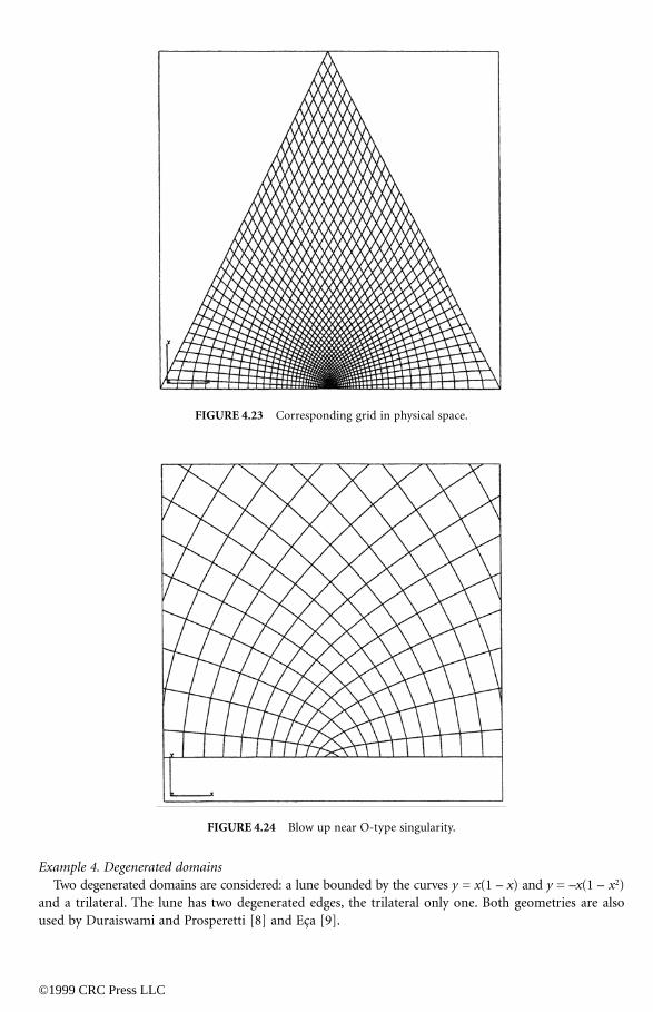
the grid obtained with Algorithm 2. The corresponding grid control map, based on Eq. 4.27 and Eq. 4.28,is shown in Figure 4.18 as a grid in parameter space P. Notice that the grid lines are straight in P. Figure 4.21shows the grid in parameter space obtained by solving ∆s = 0 and ∆t = 0 on the grid shown in Figure 4.19supplied with Neumann boundary conditions on the two bottom edges of the triangle. It should benoticed that although this grid control map is completely different from the grid control map shown inFigure 4.18, the corresponding grid in the interior of the triangle will still be the same. Figure 4.22 showsthe new grid control map based on Eq. 4.42, 4.43. Thus the position of the boundary grid points is thesame in both Figure 4.22 and Figure 4.21. Notice that the grid is orthogonal at the left and bottom edgeof P. These two edges in P correspond with the two bottom edges of the triangle. The corresponding gridis shown in Figure 4.23. The grid is clearly orthogonal at the two bottom edges of the triangle. Figure 4.23shows the nice behavior of the grid near the 0-type singularity.

FIGURE 4.14 Laplace grid.


Example 2. Circular domainThis example illustrates Algorithm 5 for complete grid control at the boundary. The prescribed

boundary grid points are evenly spaced as shown in Figure 4.26. The grid in parameter space P, basedon Eq. 4.27 and Eq. 4.28, is shown in Figure 4.25 and is thus uniform so that the corresponding grid inFigure 4.26 is a Laplace grid. Figure 4.27 shows the grid in parameter space obtained by solving ∆s = 0and ∆t = 0 supplied with Neumann boundary conditions at all four sides. Figure 4.28 shows the new

FIGURE 4.15 Grid with cell height control at upper and lower side.

FIGURE 4.16 Grid with boundary orthogonality at upper and lower side.


grid control map based on Eq. 4.42 and Eq. 4.43. This grid in parameter space is no longer uniform butremains rectangular because of the symmetry in both geometry and boundary grid. The correspondinggrid in physical space, shown in Figure 4.29, is thus orthogonal as explained in Section 4.2.3.4. Noticethe bad mesh spacing along the boundary of this orthogonal grid. The adapted grid in parameter spaceto obtain also a good mesh spacing is shown in Figure 4.30. This adapted grid is obtained by the methoddescribed in Section 4.2.3.5. Figure 4.31 shows the corresponding grid in physical space and demonstratesthe successful combination of boundary grid orthogonality and good mesh spacing.

FIGURE 4.17 Grid with both cell height control and boundary orthogonality at upper and lower side.

FIGURE 4.18 Initial grid in parameter space based on normalized arc length.


Example 3. Domain bounded by semicircles on the four sides of the unit squareThis geometry is also used by Duraiswami and Prosperetti [8] and Eça [9]. The prescribed boundary

grid points are no longer evenly spaced but dense near the four corners of the domain. Figure 4.32 showsthe grid in parameter space based on Eq. 4.27 and Eq. 4.28. Figure 4.33 shows the corresponding grid inphysical space. Figure 4.34 shows the grid in parameter space obtained by solving ∆s = 0 and ∆t = 0supplied with Neumann boundary conditions at all four sides. Figure 4.35 shows the new grid controlmap based on Eq. 4.42 and Eq. 4.43. This grid in parameter space is rectangular because of the symmetry

FIGURE 4.19 Corresponding grid in physical space.

FIGURE 4.20 Blow up near O-type singularity.


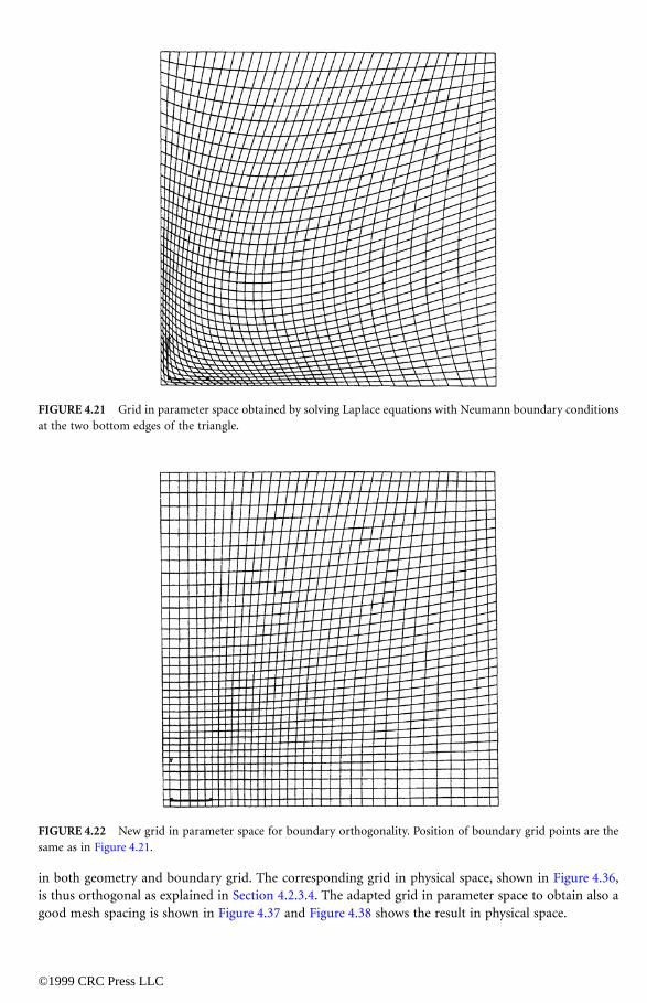
in both geometry and boundary grid. The corresponding grid in physical space, shown in Figure 4.36,is thus orthogonal as explained in Section 4.2.3.4. The adapted grid in parameter space to obtain also agood mesh spacing is shown in Figure 4.37 and Figure 4.38 shows the result in physical space.

FIGURE 4.21 Grid in parameter space obtained by solving Laplace equations with Neumann boundary conditionsat the two bottom edges of the triangle.

FIGURE 4.22 New grid in parameter space for boundary orthogonality. Position of boundary grid points are thesame as in Figure 4.21.


Example 4. Degenerated domainsTwo degenerated domains are considered: a lune bounded by the curves y = x(1 – x) and y = –x(1 – x2)

and a trilateral. The lune has two degenerated edges, the trilateral only one. Both geometries are alsoused by Duraiswami and Prosperetti [8] and Eça [9].


FIGURE 4.24 Blow up near O-type singularity.


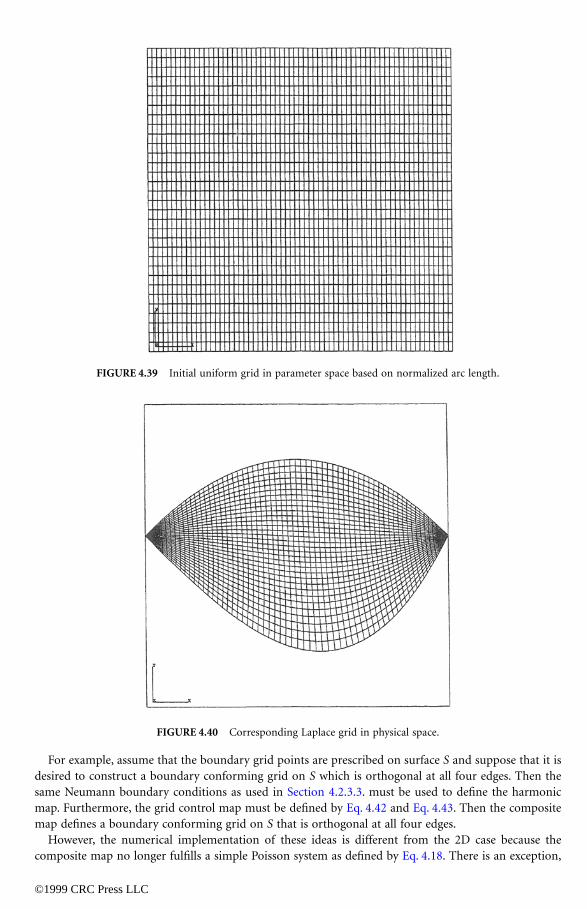
In case of the lune, an evenly spaced boundary grid point distribution is used so that the grid inparameter space based on Eq. 4.27 and Eq. 4.28 is uniform and the corresponding grid in physical spaceis harmonic. See Figure 4.39 and Figure 4.40. Figure 4.41 shows the grid in parameter space obtained bysolving ∆s = 0 and ∆t = 0 supplied with Neumann boundary conditions at the two nondegenerated edges.Notice the large change in the position of the boundary grid points in parameter space compared to theinitial uniform grid. Figure 4.42 shows the new grid control map based on Eq. 4.42 and Eq. 4.43. This

FIGURE 4.25 Initial uniform grid in parameter space based on normalized arc length.

FIGURE 4.26 Corresponding Laplace grid in physical space.


grid in parameter space is almost rectangular. The corresponding grid in physical space, shown inFigure 4.43, is therefore almost orthogonal.

For the trilateral, we show only the final grid in parameter space, obtained by Algorithm 5, and thecorresponding grid in physical space. See Figure 4.44 and Figure 4.45.

FIGURE 4.27 Grid in parameter space obtained by solving the Laplace equations with Neumann boundary con-ditions at all four sides.

FIGURE 4.28 New grid in parameter space for boundary orthogonality at all four sides. Position of boundarypoints is the same as in Figure 4.27.


Example 5. Navier–Stokes grid around a complex artificial boundaryThis example is used to demonstrate the robustness of the proposed algorithms. Figure 4.46 shows

the grid in parameter space based on Eq. 4.27 and Eq. 4.28, and Figure 4.47 shows the corresponding C-type Navier–Stokes grid in physical space. Figure 4.49 shows the grid in parameter space obtained bysolving ∆s = 0 and ∆t = 0 with Neumann boundary conditions at the lower boundary of the domain(three edges). Figure 4.50 shows the new grid in parameter space based on Eq. 4.42 and Eq. 4.43. Thegrid is orthogonal at the left, right, and lower side of the parameter space. The corresponding grid inphysical space is shown in Figure 4.51 and Figure 4.52.

FIGURE 4.29 Corresponding grid in physical space. Interior grid is also orthogonal.

FIGURE 4.30 Adapted grid in parameter space for complete boundary control.


4.3 Surface Grid Generation

The concepts of harmonic maps and grid control maps as used for grid generation in 2D domains canalso be used for grid generation on surfaces in 3D.

Consider a surface S bounded by four edges E1, E2, E3, E4. Let (E1, E2) and (E3, E4) be the two pairs ofopposite edges as shown in Figure 4.3.


FIGURE 4.32 Initial grid in parameter space based on normalized arc length.


A harmonic map is defined as a differentiable one-to-one map from S onto a unit square such that

1. The boundary of S is mapped onto the boundary of the unit square,2. The vertices of S are mapped, in the proper sequence, onto the corners of the unit square,3. The two components of the map are harmonic functions on S. This means that the two components

obey the Laplace–Beltrami equations for surfaces (see Part II of Section 2.5 in Chapter 2).


FIGURE 4.34 Grid in parameter space obtained by solving the Laplace equations with Neumann boundary con-ditions at all four sides.


Let : S a P be a harmonic map where the parameter space P is the unit square in a two-dimensionalspace with Cartesian coordinates = (s, t)T. Thus ∆s = 0 and ∆t = 0 where ∆ is the Laplace–Beltramioperator for surfaces [15].

The problem of generating an appropriate grid on surface S can be effectively reduced to a simplerproblem of generating an appropriate grid in the parameter space P, which can after that be mapped onS, by using the inverse of the harmonic map : P a S.

FIGURE 4.35 New grid in parameter space for boundary orthogonality. Position of boundary grid points are thesame as in Figure 4.34

FIGURE 4.36 Corresponding grid in physical space. Interior grid is also orthogonal.

rs

rs

rx


Define the computational space C as the unit square in a two-dimensional space with Cartesiancoordinates = (ξ, η)T A grid control map : C a P is defined as a differentiable one-to-one map fromC onto P and maps a uniform grid in C to a, in general, nonuniform grid in P.

The composition of a grid control map : C a P and the inverse of the harmonic map : P a Sdefines a map : C a S which transforms a uniform grid in C to a, in general, nonuniform grid onsurface S. The same ideas as used for 2D domains can be applied to construct appropriate grid controlmaps such that the corresponding surface grid has desired properties.

FIGURE 4.37 Adapted grid in parameter space for complete boundary control.


rξ

rs

rs

rx

rx


For example, assume that the boundary grid points are prescribed on surface S and suppose that it isdesired to construct a boundary conforming grid on S which is orthogonal at all four edges. Then thesame Neumann boundary conditions as used in Section 4.2.3.3. must be used to define the harmonicmap. Furthermore, the grid control map must be defined by Eq. 4.42 and Eq. 4.43. Then the compositemap defines a boundary conforming grid on S that is orthogonal at all four edges.

However, the numerical implementation of these ideas is different from the 2D case because thecomposite map no longer fulfills a simple Poisson system as defined by Eq. 4.18. There is an exception,

FIGURE 4.39 Initial uniform grid in parameter space based on normalized arc length.

FIGURE 4.40 Corresponding Laplace grid in physical space.


namely when S is a minimal surface. A minimal surface has zero mean curvature, and its shape is a soapfilm bounded by its four edges. There is a famous theorem in differential geometry which states that theLaplace–Beltrami operator applied on the position vector of an arbitrary surface S obeys

(4.54)

FIGURE 4.41 Grid in parameter space obtained by solving Laplace equations with Neumann boundary conditionsat the two nondegenerated edges.

FIGURE 4.42 New grid in parameter space for boundary orthogonality at the two nondegenerated edges. Positionof boundary grid points are the same as in Figure 4.41.

∆r rx Hn= 2


where is the unit vector normal to the surface and H is the mean curvature. (See Part II of Section 2.5in Chapter 2, or Theorem 1 in Dierkes, et al. [7]). The requirement of zero mean curvature implies

(4.55)

Thus for minimal surfaces we also have ∆s = 0, ∆t = 0 and ∆ = 0. Following the same derivation asin Section 4.2.1 for 2D domains, we find that the composite map obeys the same Poisson system given


FIGURE 4.44 Constructed grid in parameter space for both grid orthogonality and mesh spacing control at theboundary of a trilateral.

rn

∆rx = 0

rx


by Eq. 4.18 (for more details see [25]). Thus an interior grid point distribution on a minimal surface isfound by solving Eq. 4.18 with the prescribed boundary grid points as Dirichlet boundary conditions.The only difference compared with the two-dimensional case is that now = (x, y, z)T instead of = (x, y)T.The same ideas to construct appropriate grid control maps and their corresponding grids in 2Ddomains can also be directly applied to minimal surfaces. In fact, all previously discussed 2D examplesare generated as minimal surface grids where the four boundary edges are lying in a plane in three-dimensional space.

FIGURE 4.45 Corresponding grid in trilateral.

FIGURE 4.46 Initial grid in parameter space map based on normalized arc length.

rx

rx


Examples of characteristic minimal surface grids are shown in Figures 4.53–4.57. Figure 4.53 is a so-calledsquare Scherk surface [7]. Figure 4.54 shows what happens when the boundary edges of the Scherk surfaceare replaced by semicircular arcs. Figure 4.55 and Figure 4.56 show the change in the shape of the minimalsurface when these semicircular arcs are bent together. Boundary orthogonality is imposed at all four sidesfor all these three cases. Because of the symmetry in both geometry and boundary grid point distribution,the generated surface grids are not only orthogonal at the boundary but also in the interior. Finally, Figure 4.57is Schwarz’s P-surface [7], which is in fact constructed as a collection of connected minimal surfaces.


FIGURE 4.48 Blow up.


In general, surface S is not a minimal surface but a parametrically defined surface with a prescribedgeometrical shape given by a map : Q a S where Q is some parameter space defined as a unit squarein 2D. In order to construct, for example, a boundary conforming grid on S which is orthogonal at allfour edges, we solve on an initial surface grid on S the Laplace–Beltrami equations with the same Neumannboundary conditions as used in Section 4.2.3.3. The solution can be written as a map : Q a P. Theappropriate grid control map, defined by Eq. 4.42 and Eq. 4.43, defines a nonuniform grid in P. Thecorresponding grid in Q can then be found by using the inverse map –1: P a Q. This is done numerically

FIGURE 4.49 Solution of Laplace equations with Neumann boundary conditions at the three bottom edges of thedomain.

FIGURE 4.50 New grid in parameter space for boundary orthogonality at the three bottom edges of the domain.Position of the boundary grid points is the same as in Figure 4.49.

rx

rs

rs


in a way described in [25]. Once the corresponding grid in Q is found, then the corresponding surfacegrid on S is computed using the parametrization : Q a S. This new surface grid on S differs from theinitial surface grid S. The complete process should be repeated until the surface grid on S (and thecorresponding grids in parameter space P and Q) do not change anymore. In practice, only a few(Eq. 4.2–4.5) iterations appear to be sufficient. After convergence, the final surface grid not only isor-thogonal at the boundary but is also independent of the parametrization and depends only on the shapeof the surface and the position of the boundary grid points.


FIGURE 4.52 Blow up.

rx


4.4 Volume Grid Generation

Consider a simply connected bounded domain D in three-dimensional space with Cartesian coordinates = (x, y, z)T. Suppose that D is bounded by six faces Fl, F2, F3, F4, F5, F6. Let (F1, F2), (F3, F4), and (F5,

F6) be the three pairs of opposite faces. Furthermore, consider the 12 edges {Ei, i = 1 … 12} and assumethat these edges are related to the six faces as shown in Figure 4.4.

FIGURE 4.53 Minimal surface grid (Scherk surface). Surface grid is orthogonal.

FIGURE 4.54 Minimal surface grid bounded by four orthogonal circular arcs. Surface grid is orthogonal.

rx


In 3D, a harmonic map is defined as a differentiable one-to-one map from D onto a unit cube such that

1. The boundary of D is mapped onto the boundary of the unit cube,2. The vertices, edges, and faces of D are mapped onto the corresponding vertices, edges, and faces

of the unit cube,3. The three components of the map are harmonic functions in the interior of D.

FIGURE 4.55 Change in shape by bending opposite circular arcs together.

FIGURE 4.56 Projection on xy-plane.


Let : D a P be a harmonic map where the parameter space P is the unit cube in a three-dimensionalspace with Cartesian coordinates = (s, t, u)T. Inside D the components obey

(4.56)

Define the computational space C as the unit cube in a three-dimensional space with Cartesian coordi-nates = (ξ, η, ζ )T. A grid control map : C a P is defined as a differentiable one-to-one map from Conto P and maps a uniform grid in C to a, in general, nonuniform grid in P.

The composition of a grid control map : C a P and the inverse of the harmonic map : P a Ddefines a map : C a D that transforms a uniform grid in C to a, in general, nonuniform grid in D. Asin 2D, the composite map obeys a quasi-linear system of elliptic partial differential equations, known asthe Poisson grid generation equations, with control functions completely defined by the grid control map.

The derivation of the Poisson grid generation equations can be done along the same lines as for the2D case. Suppose that the harmonic map and grid control map are defined so that the composite mapexists. Introduce the three covariant base vectors

(4.57)

and the covariant metric tensor components

(4.58)

The three contravariant base vectors 1 , 2 , and3 obey

FIGURE 4.57 Schwarz’s P-minimal surface.

rs

rs

∆ ∆ ∆s s s s t t t t u u u uxx yy zz xx yy zz xx yy zz= + + = = + + = = + + =0 0 0

rξ

rs

rs

rx

rx

r r r r rx a x a x1 2 3= = =ξ η ζ

a a aij i j= ( )r r

, i = {1,2,3} j = {1,2,3}

ra ∇ x xx xy xz, ,( )T= =

ra ∇ h hx hy hz, ,( )T= =

ra ∇ z zx zy zz, ,( )T= =

(4.59)

r ra a i ji

j ji, { , , } { , , }( ) = = =δ 1 2 3 1 2 3


Define the contravariant metric tensor components

(4.60)

so that

(4.61)

Define J2 as the determinant of the covariant metric tensor.Consider an arbitrary function . Then is also defined in domain D and the Laplacian

of can be expressed as

(4.62)

As in the two-dimensional case, substitution of and φ≡ζ into this equation yieldsexpressions for ∆ξ, ∆η, and ∆ζ. Combining these expressions with Eq. 4.62 gives

(4.63)

Substitute = (s, t, u)T in Eq. 4.63 and use the property that s, t, and u are harmonic in domain D, i.e.,∆s = 0, ∆t = 0, and ∆u = 0. Then the following expressions for the Laplacian of ξ, η, and ζ are found:

(4.64)

where

(4.65)

a a a i jij i jr r

, { , , } { , , }( ) = = 1 2 3 1 2 3

a a a

a a a

a a a

a a a

a a a

a a a

11 12 13

12 22 23

13 23 33

11 12 13

12 22 23

13 23 33

1

0

0

0 0

1 0

0 1

=

f f x h z, ,( )= ff

∆φ φ φ φ φ φ φ

φ φ φ

ξ η ζ ξ ξ η ζ η

ξ η ζ ζ

= + +( ) + + +( )+ + +( )

1 11 12 13 12 22 23

13 23 33

JJa Ja Ja Ja Ja Ja

Ja Ja Ja

{ }

}

f x f h≡,≡

∆ ∆ ∆ ∆φ φ φ φ φ φ φ ξφ ηφ ζφξξ ξη ξζ ηη ηζ ζζ ξ η ζ= + + + + + + + +a a a a a a11 12 13 22 23 332 2 2

f

∆∆∆

ξηζ

= + + + + +a P a P a P a P a P a P1111

1212

1313

2222

2323

33332 2 2

r r r r r r

r r r

r r

P T

s

t

u

P T

s

t

u

P T

s

t

u

P T

s

t

u

P

111

121

131

221

23

= −

= −

= −

= −

= −

− − −

−

ξξ

ξξ

ξξ

ξη

ξη

ξη

ξζ

ξζ

ξζ

ηη

ηη

ηη

TT

s

t

u

P T

s

t

u

− −

= −

133

1ηζ

ηζ

ηζ

ζζ

ζζ

ζζ

r

and the matrix T is defined as


(4.66)

The 18 coefficients of the six vectors 11, 12, 13, 22, 23, 33, are so-called control functions. Thus the18 control functions are completely defined and easily computed for a given grid control map = ( ).

Finally, substituting φ ≡ in Eq. 4.63 and using the fact that ∆ ≡ 0, we arrive at the following equation:

(4.67)

The final form of the Poisson grid generation system can now be derived from this equation by substitu-tion of Eq. 4.64, by multiplication with J2, and by expressing the contravariant tensor components in thecovariant tensor components according to Eq. 4.61. The result can be written as

(4.68)

with

(4.69)

and

(4.70)

This equation, together with the expressions for the control functions Pkij given by Eq. 4.65, forms the

3D grid generation system. For a given grid control map, so that the 18 control functions in Eq. 4.68 aregiven functions of (ξ, η, ζ ), boundary conforming grids in the interior of domain D are computed bysolving this quasi-linear system of elliptic partial differential equations with prescribed boundary gridpoints as Dirichlet boundary conditions.

The construction of appropriate grid control maps for 3D domains is less well developed than for 2Ddomains. In [25], a grid control map has been proposed which works surprisingly well for manyapplications. The grid control map is the 3D extension of the 2D grid control map defined by Eq. 4.27and Eq. 4.28. The map : C a P is defined by

(4.71)

T

s s s

t t t

u u u

ξ η ζ

ξ η ζ

ξ η ζ

rP

rP

rP

rP

rP

rP

rs

rs

rξr

xrx

a x a x a x a x a x a x x x x11 12 13 22 23 332 2 2 0

r r r r r r r r rξξ ξη ξζ ηη ηζ ζζ ξ η ζξ η ζ+ + + + + + + + =∆ ∆ ∆

a x a x a x a x a x a x

a P a P a P a P a P a P x

a P a P a P a

11 12 13 22 23 33

11111 12

121 13

131 22

221 23

231 33

331

11112 12

122 13

132 22

2 2 2

2 2 2

2 2

r r r r r r

rξξ ξη ξζ ηη ηζ ζζ

ξ

+ + + + +

+ + + + + = + + =( )+ + + + + = PP a P a P x

a P a P a P a P a P a P x

222 23

232 33

332

11113 12

123 13

133 22

223 23

233 33

333

2

2 2 2 0

+ + =( )+ + + + + = + + =( ) =

r

r

η

ζ

a a a a a a a a a a a a a a

a a a a a a a a a a a a a

1122 33 23

2 1213 23 12 33

1312 23 13 22

2211 33 13

2 2313 12 11 23

3311 22 12

2

= − = − = −

= − = − = −

a x x a x x a x x

a x x a x x a x x

11 12 13

22 23 33

= ( ) = ( ) = ( )= ( ) = ( ) = ( )

r r r r r r

r r r r r r

ξ ξ ξ η ξ ζ

η η η ζ ζ ζ

, , ,

, , ,

rs

s s t u s t u s t u s tuE E E E= ( ) −( ) −( ) + ( ) −( ) + ( ) −( ) + ( )1 2 3 4

1 1 1 1ξ ξ ξ ξ


(4.72)

(4.73)

where the twelve edge functions sE1, …, uE12

measure the normalized arc length along the correspondingtwelve edges of domain D (see Figure 4.4).

Equation 4.71 implies that a grid plane ξ = const. is mapped to the parameter space P as a bilinearsurface: s is a bilinear function of t and u. Similarly, Eq. 4.72 and Eq. 4.73 imply that grid planes η =const. and ζ = const. are also mapped to the parameter space P as bilinear surfaces. For a givencomputational coordinate (ξ, η, ζ ) the corresponding (s, t, u) value is found as the intersection pointof three bilinear surfaces. Newton iteration is used to compute the intersection points. It can be easilyverified that two bilinear surfaces corresponding to two different ξ-values will never intersect in parameterspace P. The same is true for two different η or ζ values. This observation indicates that the grid controlmap is a differentiable one-to-one mapping.

An illustration of a volume grid computed by solving Eq. 4.68, with the grid control map defined byEq. 4.71–4.73, is shown in Figures 4.58–4.61. The domain is a semi-torus. The prescribed boundary gridpoints on the surface of the semi-torus are shown in Figure 4.58. Figure 4.59 shows the surface grid onthe two exterior circular grid planes. Figure 4.60 shows the computed interior grid depicted on someinternal circular planes. Figure 4.61 shows the computed interior grid on the circular plane exactly halfwayinside the torus. The mesh spacing of the interior grid is excellent despite the concave boundary. Theangles between the interior grid lines and the boundary surface are reasonable but no longer orthogonal.This is not surprising, because the grid control map provides no control about the angle distributionbetween interior grid lines and the boundary of the domain.

FIGURE 4.58 Boundary surface grid of a semi-torus.

t t s u t s u t s u t suE E E E= ( ) −( ) −( ) + ( ) −( ) + ( ) −( ) + ( )5 6 7 8

1 1 1 1η η η η

u u s t u s t u s t u stE E E E= ( ) −( ) −( ) + ( ) −( ) + ( ) −( ) + ( )9 10 11 12

1 1 1 1ζ ζ ζ η


4.5 Research Issues and Summary

The grid generation systems of elliptic quasi-linear second-order partial differential equations are thefamiliar so-called Poisson systems with control functions to be specified. In this chapter, a Poisson systemis considered as a system of partial differential equations that the composition of a grid control map andthe inverse of a harmonic map has to obey. The control functions in the Poisson system are thencompletely defined by the grid control map. Boundary conforming grids in physical space are computedby solving the Poisson system with control functions specified by a grid control map.

FIGURE 4.59 Surface grid on the two exterior circular planes.

FIGURE 4.60 Interior grid planes inside the torus.


One of the main advantages of this approach is that the method is noniterative. If an appropriate gridcontrol map has been constructed, then the corresponding grid control functions of the Poisson systemare computed and their values remain unchanged during the solution of the Poisson system. Anotheradvantage is that the construction of an appropriate grid control map can be considered as a numericalimplementation of the constructive proof for the existence of the desired grid in physical space. If thegrid control map is one-to-one, then the composition of the grid control map and the inverse of theharmonic maps exist so that the solution of the Poisson system is well-defined.

In two dimensions, boundary orthogonality is obtained by applying Dirichlet–Neumann boundaryconditions for the harmonic map. In that case, the harmonic map is quasi-conformal. This propertyshows the relation with orthogonal grid generation.

The use of harmonic maps and grid control maps for surface grid generation is also shortly described.The two-dimensional Poisson systems can be directly extended to surface grid generation on minimalsurfaces (soap films). The extension to volume grid generation is also given.

The construction of appropriate grid control maps such that the corresponding grid in physical spacehas desired properties is the main issue of this chapter. The chosen examples concern mainly simple well-defined geometries so that the reader is able to recompute the grids. However, the elliptic grid generationmethods described in this chapter have been implemented in ENGRID, NLR’s multi-block grid generationcode [26,27,2], and are nowadays used on a routine basis to construct Euler or Navier–Stokes grids inblocks and block-faces with complex geometrical shapes. The construction of appropriate grid controlmaps for 3D domains is less well developed than for 2D domains and surfaces. Further investigation isexpected in this direction.

4.6 Further Information

The book of Thompson, Warsi, and Mastin [30] is still the best introduction to elliptic grid generationsystems. A more recent book is Carey [4]. Also the book of Knupp and Steinberg [14] is a valuable sourceabout the fundamentals of structured grid generation and related topics, like tensor analysis and differ-ential geometry. The book of Kreyszig [15] and Dierkes, et.al. [7] are excellent textbooks about differentialgeometry and tensor analysis.

FIGURE 4.61 Interior grid inside the torus on a circular plane halfway between the two exterior circular planes.

The proceedings of the grid generation conferences [1,22,33], the VKI lecture series about grid gen-eration [31,32], and the NASA conference publications [5,6] contain a lot of useful information about


the application of elliptic grid generation systems, often embedded in multiblock grid generation systems.The Journal of Computational Physics provides many good more or less fundamental articles about

elliptic grid generation systems.

References

1. Arcilla, A. S., (Ed.) et al., Numerical grid generation in computational fluid dynamics and relatedfields, Proceedings of the 3rd International Conference, Barcelona, Spain, North-Holland, 1991.

2. Boerstoel, J. W., Kassies, A., Kok, J. C., and Spekreijse, S. P., ENFLOW — a full-functionalitysystem of CFD codes for industrial Euler/Navier–Stokes flow computations, Proceedings of 2ndInternational Symposium on Aeronautical Science and Technology, IASTTI’96, Jakarta, Indonesia,1996.

3. Bjorstad, P. E., Numerical solution of the biharmonic equation, Ph.D. thesis, Stanford University,1980.

4. Carey, G. F., Computational Grids, Taylor & Francis, 1997.5. Chawner, J. R. and Steinbrenner, J. P., Automatic Structured Grid Generation using GRIDGEN,

Surface Modeling, Grid Generation, and Related Issues in Computational Fluid Dynamic (CFD)Solutions, Choo, Y. K., (Ed.), NASA-CP-3291, 1995, pp. 463–476.

6. Choo, Y. K., (Ed.), Surface Modeling, Grid Generation, and Related Issues in Computational FluidDynamic (CFD) Solutions, NASA-CP-329 1, Proceedings of a workshop held at NASA Lewis,Cleveland, Ohio, 1995.

7. Dierkes, U., Hildebrandt, S., Kuster, A., and Wohlrab, O., Minimal surfaces I, Grundlehren derMathematischen Wissenschaffen 295, Springer Verlag, Berlin, 1991.

8. Duraiswami, R. and Prosperetti, A., Orthogonal mapping in two dimensions, J.Comput. Phys.,98, pp. 254–268, 1992.

9. Eça, L., 2D orthogonal grid generation with boundary point distribution control, J. Comput. Phys.,125, pp. 440–453, 1996.

10. Farin, G., Curves and Surfaces for Computer Aided Geometric Design — A Practical Guide. AcademicPress, San Diego, 1990.

11. Henrici, P., Applied and Computational Complex Analysis, Vol. 3, Wiley, New York, 1986.12. Hsu, K. and Lee, S.L., A numerical technique for two-dimensional grid generation with grid control

at all of the boundaries, J.Comput. Phys., 96, pp. 451–469, 1991.13. Kang, I.S. and Leal, L.G., Orthogonal grid generation in a 2D domain via the boundary integral

technique, J. Comput. Phys., 102, pp. 78–87, 1992.14. Knupp, P. and Steinberg, S., Fundamentals of Grid Generation, CRC Press, Boca Raton, FL, 1993.15. Kreyszig, E., Differential Geometry, Dover, New York, 1991.16. Mastin, C. W., Multilevel elliptic smoothing of large three-dimensional grids, Surface Modeling,

Grid Generation, and Related Issues in Computational Fluid Dynamic (CFD) Solutions, Choo, Y. K,(Ed.), NASA-CP-3291, pp. 689–696, 1995.

17. Oh, H. J. and Kang, I. S., A non-iterative scheme for orthogonal grid generation with controlfunction and specified boundary correspondence on three sides, J. Comput. Phys., 112, pp. 138–148, 1994.

18. Roache, P. J. and Steinberg, S., A new approach to grid generation using a variational formulation,AIAA 7th Computational Fluid Dynamics Conference, AIAA paper 85-1527, pp. 360–370, 1985.

19. Ryskin, G. and Leal, L. G., Orthogonal mapping, J. Comput. Phys., 50, pp. 71–100, 1983.20. Smith, R. E., (Ed.), Software systems for surface modeling and grid generation, NASA-CP-3143,

Proceedings of a workshop held at NASA Langley, Hampton, VA, 1992.21. Sonar, T., Grid generation using elliptic partial differential equations, DFVLR Forschungsbericht

89–15, 1989.

22. Soni, B. K., (Ed.), et al., Numerical grid generation in computational field simulations, Proceedingsof the 5th International Conference, Mississippi State University, NSF Engineering Research Center


for Computational Field Simulation, 1996.23. Sorenson, R. L. and Alter, S. J., 3D GRAPE/AL: The Ames/Langley technology update, Surface

Modeling, Grid Generation, and Related Issues in Computational Fluid Dynamic (CFD) Solutions,Choo, Y. K., (Ed.), NASA-CP-3291, pp 447–462, 1995.

24. Sorenson, R. L. and Steger, J. L., Numerical Generation of Two-Dimensional Grids by Use ofPoisson Equations with Grid Control, Numerical Grid Generation Techniques, Smith, R. E., (Ed.),NASA-CP-2166, pp. 449–461, 1980.

25. Spekreijse, S. P., Elliptic grid generation based on Laplace equations and algebraic transformations,J. Comput. Phys., 118, pp. 38–61, 1995.

26. Spekreijse, S. P. and Boerstoel, J. W., Multiblock grid generation, Part 1: Elliptic grid generationmethods for structured grids, Computational Fluid Dynamics, VKI-Lecture-Series 1996-06, Decon-inck, H., (Ed.), Von Karman Institute for Fluid Dynamics, pp. 1–39, 1996.

27. Spekreijse, S. P. and Boerstoel, J. W., Multiblock Grid Generation, Part 2: Multiblock Aspects,Computational Fluid Dynamics, VKI-Lecture-Series 1996-06, Deconinck, H., (Ed.), Von KarmanInstitute for Fluid Dynamics, pp. 1–48, 1996.

28. Takahashi, S. and Eiseman P. R., Adaptive grid movement with respect to boundary curvature,Numerical Grid Generation in Computational Fluid Dynamics and Related Fields, 4th InternationalGrid Conference, Weatherill N. P., et al. (Eds.), Pineridge Press Limited, Swansea, Wales (UK),1994,p. 563.

29. Thompson, J. E., A composite grid generation code for general 3D regions — the EAGLE code,AIAA Journal, 1988, 26, Vol.3, p 271.

30. Thompson, J. F., Warsi, Z.U.A., and Mastin, C.W., Numerical Grid Generation: Foundations andApplications, Elsevier, New York, 1985.

31. Weatherill, N. P., (Ed.), Grid generation, VKI-Lecture-Series 1994-02, Von Karman Institute forFluid Dynamics, 1994.

32. Weatherill, N. P., (Ed.), Numerical grid generation, VKI-Lecture-Series 1990-06, Von KarmanInstitute for Fluid Dynamics, 1990.

33. Weatherill, N. P., (Ed.), et al., Numerical Grid Generation in Computational Fluid Dynamics andRelated Fields, Proceedings of the 4th International Conference, Swansea, Wales, Pineridge Press,1994.

34. Winslow, A., Numerical solution of the quasilinear poisson equations in a nonuniform trianglemesh, J. Comput. Phys., 2, pp. 149–172, 1967.

35. Warsi, Z. U. A., Basic differential models for coordinate generation, Proceedings Numerical GridGeneration. Thompson, J. F. (Ed.), North-Holland, Amsterdam, pp. 41–77, 1982.

36. Yamaguchi, F., Curves and Surfaces in Computer Aided Geometric Design, Springer Verlag, Berlin,1988.

Chapter 4: Elliptic Generation Systems - Freeebrary.free.fr/Mesh Generation/Handbook_of_Grid_...

Documents

Transcript of Chapter 4: Elliptic Generation Systems - Freeebrary.free.fr/Mesh Generation/Handbook_of_Grid_...