CHAPTER 4 COMPARING MEANS USING THE...

Chapter 5: Comparing two means using the t-test

1

CCChhhaaapppttteeerrr 555:::

CCCOOOMMMPPPAAARRRIIINNNGGG TTTWWWOOO MMMEEEAAANNNSSS UUUSSSIIINNNGGG TTTHHHEEE TTT---TTTEEESSSTTT

Upon completion of this chapter, you should be able to:

explain what is the t-Test and its use in hypothesis testing

demonstrate using the t-Test for INDEPENDENT MEANS

identify the assumptions for using the t-test

demonstrate the use of the t-Test for DEPENDENT MEANS

CHAPTER OVERVIEW

What is the t-test?

The hypothesis tested using the t-

test

Using the t-test for independent

means

Assumptions that must be observed

when using the t-test

Summary

Key Terms

References

Chapter 1: Introduction

Chapter 2: Descriptive Statistics

Chapter 3: The Normal Distribution

Chapter 4: Hypothesis Testing

Chapter 5: T-test

Chapter 6: Oneway Analysis of Variance

Chapter 7: Correlation

Chapter 8: Chi-Square

This chapter introduces you to the t-test which is statistical tool used to test the significant

differences between the means of two groups. The independent t-test is used when the

means of two groups when the sample is drawn from two different or independent

samples. The dependent or pairwise t-test is used when the sample is tested twice the

means are compared.


2

What is the T-Test?

The t-test was developed by a statistician, W.S.

Gossett (1878-1937) who worked in a brewery in Dublin,

Ireland. His pen name was ‘student’ and hence the term

‘student’s t-test’ which was published in the scientific

journal, Biometrika in 1908. The t-test is a statistical tool

used to infer differences between small samples based on

the mean and standard deviation.

In many educational studies, the researcher is

interested in testing the differences between means on

some variable. The researcher is keen to determine

whether the differences observed between two samples

represents a real difference between the populations from

which the samples were drawn. In other words, did the observed difference just

happen by chance when, in reality, the two populations do not differ at all on the

variable studies.

or example, a teacher wanted to find out whether the Discovery method of

teaching science to primary school children was more effective than the Lecture

method. She conducted an experiment among 70 primary school children of which 35

pupils were taught using the Discovery method and 35 children were taught using the

Lecture method. The results of the study showed that subjects in the Discovery group

scored 43.0 marks while subjects in the Lecture method group score 38.0 marks on a

the science test. Yes, the Discovery group did better than the Lecture group. Does the

difference between the two groups represent a real difference or was it due to

chance? To answer this question, the t-test is often used by researchers.


3

The Hypothesis Tested Using the T-Test

How do we go about establishing whether the differences in the two means are

statistically significant or due to chance? You begin by formulating a hypothesis

about the difference. This hypothesis states that the two means are equal or the

difference between the two means is zero and is called the null hypothesis.

Using the null hypothesis, you begin testing the significance by saying:

"There is no difference in the score obtained in science between subjects in the

Discovery group and the Lecture group".

More commonly the null hypothesis may be stated as follows:

a) Ho : U1 = U2 which translates into 43.0 = 38.0

b) Ho : U1 ─ U2 = 0 which translate into 43.0 ─ 38.0 = 0

If you reject the null hypothesis, it means that the difference between the two

means have statistical significance

If you do not reject the null hypothesis, it means that the difference between

the two means are NOT statistically significant and the difference is due to

chance.

Note:

For a null hypothesis to be accepted, the difference between the two means need not

be equal to zero since sampling may account for the departure from zero. Thus, you

can accept the null hypothesis even if the difference between the two means is not

zero provided the difference is likely to be due to chance. However, if the difference

between the two means appears too large to have been brought about by chance, you

reject the null hypothesis and conclude that a real difference exists.

LEARNING ACTIVITY

a) State TWO null hypothesis in your area of interest

that can be tested using the t-test.

b) What do you mean when you reject or do not reject

the null hypothesis?


4

Using the T-Test for INDEPEDENT MEANS

The t-test is a powerful statistic that enables you to determine that the

differences obtained between two groups is statistically significant. When two groups

are INDEPENDENT of each other; it means that the sample drawn came from two

populations. Other words used to mean that the two groups are independent are

"unpaired" groups and "unpooled” groups.

a) What is meant by Independent Means or Unpaired Means?

Say for example you conduct a study to determine the spatial reasoning ability

of 70 ten-year old children in Malaysia. The sample consisted of 35 males and 35

females. See figure 5.1. The sample of 35 males was drawn from the population of ten

year old males in Malaysia and the sample of 35 females was drawn from the

population of ten year olds females in Malaysia.

Note that they are independent samples because they come from two completely

different populations.

Figure 5.1 Samples drawn from two independent populations

Population of ten year old

MALES in Malaysia

Population of ten year old

FEMALES in Malaysia

Sample of 35 MALES

Sample of 35 FEMALES

Research Question:

"Is there a significant difference in spatial reasoning between male and female ten

year old children?"

Null Hypothesis or Ho:

"There is no significant difference in spatial reasoning between male and female

ten year old children"


5

b) Formula for the Independent T-Test

Note that the formula for the t-test shown below is a ratio. It is Group 1 mean (i.e.

males) minus Group 2 mean (i.e. females) divided by the Standard Error multiplied by

Group 1 mean minus Group 2 mean.

Computation of the Standard Error

Use the formula below. To compute the standard error (SE), you take the variance

(i.e. standard deviation squared) for Group 1 and divide it by the number of subjects

in that group minus "1". Do the same for Group 2. Than add these two values and take

the square root.

The top part of the equation is the

difference between the two means

The bottom part of the equation is

the Standard Error (SE) which is a

measure of the variability of

dispersion of the scores.

This is the formula for the

Standard Error:

Combine the two

formulas and you get

this version of the t-test

formula:


6

b) Example:

The results of the study are as follow:

Let's try using the formula:

t =

2

= ------------- = 4.124

0.485

Note: The t-value will be positive if the mean for Group I is larger or more than (>) the

mean of Group 2 and negative if it is smaller or less than (<).

c) What do you do after computing the t-value?

Once you compute the t-value (which is 4.124) you look up the t-value in The

Student's t-test Probabilities or The Table of Critical Values for Student’s T-Test

which tells us whether the ratio is large enough to say that the difference between the

groups is significant. In other words the difference observed is not likely due to

chance or sampling error.

Alpha Level: As with any test of significance, you need to set the alpha level.

In most educational and social research, the "rule of thumb" is to set the alpha

level at .05. This means that 5% of the time (five times out of a hundred) you

would find a statistically significant difference between the means even if

there is none ("chance").

Degrees of Freedom: The t-test also requires that we determine the degrees of

freedom (df) for the test. In the t-test, the degrees of freedom is the sum of the

subjects or persons in both groups minus 2. Given the alpha level, the df, and

the t-value, you look up in the Table (available as an appendix in the back of

12 -10

4.0 1

0.1177 + 0.1177

4.0 2

(35-1)

(35-1)

2

=

+


7

most statistics texts) to determine whether the t-value is large enough to be

significant.

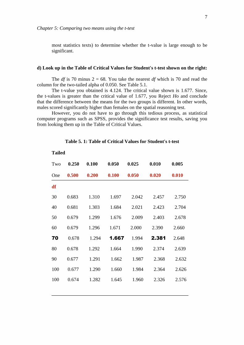
d) Look up in the Table of Critical Values for Student's t-test shown on the right:

The df is 70 minus 2 = 68. You take the nearest df which is 70 and read the

column for the two-tailed alpha of 0.050. See Table 5.1.

The t-value you obtained is 4.124. The critical value shown is 1.677. Since,

the t-values is greater than the critical value of 1.677, you Reject Ho and conclude

that the difference between the means for the two groups is different. In other words,

males scored significantly higher than females on the spatial reasoning test.

However, you do not have to go through this tedious process, as statistical

computer programs such as SPSS, provides the significance test results, saving you

from looking them up in the Table of Critical Values.

Table 5. 1: Table of Critical Values for Student's t-test

Tailed

Two 0.250 0.100 0.050 0.025 0.010 0.005

One 0.500 0.200 0.100 0.050 0.020 0.010

df

30 0.683 1.310 1.697 2.042 2.457 2.750

40 0.681 1.303 1.684 2.021 2.423 2.704

50 0.679 1.299 1.676 2.009 2.403 2.678

60 0.679 1.296 1.671 2.000 2.390 2.660

70 0.678 1.294 1.667 1.994 2.381 2.648

80 0.678 1.292 1.664 1.990 2.374 2.639

90 0.677 1.291 1.662 1.987 2.368 2.632

100 0.677 1.290 1.660 1.984 2.364 2.626

100 0.674 1.282 1.645 1.960 2.326 2.576


8

Assumptions that Must be Observed when Using the T-Test

While the t-test has been described as a robust statistical tool, it is based on a

model that makes several assumptions about the data that must be met prior to

analysis. Unfortunately, students conducting research tend not to report whether their

data meet the assumptions of the t-test. These assumptions need are be observed,

because the accuracy of your interpretation of the data depends on whether

assumptions are violated. The following are three main assumptions that are generic

to all t-tests.

Instrumentation (Scale of Measurement) The data that you collect for the dependent variable should be based on an

instrument or scale that is continuous or ordinal. For example, scores that

you obtain from a 5-point Likert scale; 1,2,3,4,5 or marks obtained in a

mathematics test, the score obtained on an IQ test or the score obtained on

an aptitude test.

Random Sampling The sample of subjects should be randomly sampled from the population

of interest.

Normality The data come from a distribution that has one of those nice bell-shaped

curves known as a normal distribution. Refer to Chapter 3: The Normal

Distribution which provides both graphical and statistical methods for

assessing normality of a sample or samples.

Sample Size

Fortunately, it has been shown that if the sample size is reasonably large,

quite severe departures from normality do not seem to affect the

LEARNING ACTIVITY

a) Would you reject Ho if you had set the alpha at 0.01 for a

two-tailed test?

b) When do you use the one-tailed test and two-tailed t-test?


9

conclusions reached. Then again what is a reasonable sample size? It has

been argued that as long as you have enough people in each group

(typically greater or equal to 30 cases) and the groups are close to equal in

size, you can be confident that the t-test will be a good, strong tool for

getting the correct conclusions. Statisticians say that the t-test is a "robust"

test. Departure from normality is most serious when sample sizes are

small. As sample sizes increase, the sampling distribution of the mean

approaches a normal distribution regardless of the shape of the original

population.

Homogeneity of Variance.

It has often been suggested by some researchers that homogeneity of

variance or equality of variance is actually more important than the

assumption of normality. In other words, are the standard deviations of the

two groups pretty close to equal? Most statistical software packages

provide a "test of equality of variances" along with the results of the t-test

and the most common being Levene's test of homogeneity of variance

(see Table 5.2).

Levene's Test 95% Confidence

of Equality Interval

of Variances

F Sig t d Sign. Mean Std. Error Upper Lower

Two-tail Difference Difference

Equal

Variances 3.39 .080 .848 20 .047 1.00 1.18 -1.46 3.46

Assumed

Unequal

Variances .848 16.70 .049 1.00 1.18 -1.49 3.40

Assumed

Table 5.2 Levene’s Test of Equality of Variances

Begin by putting forward the null hypothesis that:

"There are no significant differences between the variances of the two

groups" and you set the significant level at .05.


10

If the Levene statistic is significant, i.e. LESS than .05 level (p < .05), then the null

hypothesis is:

REJECTED and one accepts the alternative hypothesis and conclude that

the VARIANCES ARE UNEQUAL. [The unequal variances in the SPSS

output is used]

If the Levene statistic is not significant, i.e. MORE than .05 level (p > .05),

then you DO NOT REJECT (or Accept) the null hypothesis and conclude

that the VARIANCES ARE EQUAL. [The equal variances in the SPSS

output is used]

The Levene test is robust in the face of departures from normality. The Levene's test

is based on deviations from the group mean.

SPSS provides two options'; i.e. "homogeneity of variance assumed" and

"homogeneity of variance not assumed" (see Table below).

The Levene test is more robust in the face of non-normality than more

traditional tests like Bartlett's test.

Let’s examine an EXAMPLE:

In the CoPs Project, an Inductive Reasoning scale consisting of 11 items was

administered to 946 eighteen year. One of the research questions put forward is:

"Is there a significant difference between in inductive reasoning between

male and female subjects"?

To establish the statistical significance of the means of these two groups, the t-

test was used. Using SPSS.

LEARNING ACTIVITY

Refer to the table above. Based on the Levene’s Test of

Homogeneity of variance, what is your conclusion. Explain.


11

THE SPSS STEPS to answer the Research Question.

SPSS OUTPUTS:

Output #1:

The ‘Group statistics’ table above reports that the mean values on the variable

(inductive reasoning) for the two different groups (males and females). Here, we see

that the 495 females in the sample scored 8.99 while the 451 males had a mean score

of 7.95 on inductive reasoning. The standard deviation for the males is 3.46 while

that for the females is 3.14. The scores for the females are less dispersed compared to

the males.

SPSS PROCEDURES for the independent groups t-test: 1. Select the Analyze menu.

2. Click on Compare Means and then Independent- Samples T Test ....to open the Independent Samples T Test dialogue box.

3. Select the test variable(s). [i.e. Inductive Reasoning] and then click on the button to move the variables into the Test Variables(s): box 4. Select the grouping variables [i.e. gender] and click on the button to move the variable into the Grouping Variable: box

5. Click on the Define Groups ....command pushbutton to open the Define Groups sub-dialogue box.

6. In the Group 1: box, type the lowest value for the variable [i.e. 1 for 'males'], then tab. Enter the second value for the variables [i.e. 2 for 'females'] in the Group 2: box.

7. Click on Continue and then OK.


12

GROUP STATISTICS

The question remains: Is this sample difference in inductive reasoning large

enough to convince us that there it is a real significant difference in inductive

reasoning ability between the population 18 year old females and the population of 18

year-old males?

Output #2: Let’s examine this output in two parts:

First is to determine that the data meet the "Homogeneity of Variance" assumption

you can use the Levene's Test and set the alpha at 0.05. The alpha obtained is 0.054

which is greater (>) than 0.05 and you do not Reject the Ho: and conclude that the

variances are equal. Hence, you have not violated the "Homogeneity of Variance"

assumption.

Levene's Test 95% Confidence

of Equality Interval

of Variances

F Sig t d Sign. Mean Std. Error Upper Lower

Two-tail Difference Difference

Equal

Variances 4.720 .030 -4.875 944 .000 -1.0468 -2.147 -1.4682 -.6254

Assumed

Unequal

Variances -4.853 911.4 .049 -1.0468 -2.146 -1.4701 -.6234

Assumed

INDUCTIVE N Mean Std. Deviation Std. Error Mean

GENDER Male 451 7.9512 3.4618 2.345

Female 495 8.9980 3.1427 3.879


13

SECOND is to examine the following:

The SPSS output below displays the results of the t-test to test whether or not

the difference between the two sample means is significantly different from

zero.

Remember the null hypothesis states that there is no real difference between

the means (Ho: X1 = X2).

Any observed difference just occurred by chance.

Interpretation:

t-value

This "t" value tells you how far away from 0, in terms of the number of standard

errors, the observed difference between the two sample means falls. The "t" value is

obtained by dividing the difference in the Means ( - 1.0468) by the Std. Error (-.2147)

which is equal to - 4.875

p-value

If the p-value as shown in the "sig (2 tailed) column is smaller than your chosen alpha

level you do not reject the null hypothesis and argue that there is a real difference

between the populations. In other words, we can conclude, that the observed

difference between the samples is statistically significant.

Mean Difference

This is the difference between the means (labelled "Mean Difference"); i.e. 7.9512 –

8.9980 = – 1.0468.


14

Using the T-Test for Dependent Means

The Dependent means t-test or the Paired t-test or the Repeated measures

t-test is used when you have data from only one group of subjects. i.e. each subject

obtains two scores under different conditions. For example, when you give a pre-test

and after a particular treatment or intervention you give the same subjects a post-test.

In this form of design, the same subjects obtain a score on the pretest and, after some

intervention or manipulation obtain a score on the posttest. Your objective is to

determine whether the difference between means for the two sets of scores is the same

or different.

You want to find answers to the following:

Research Questions:

Is there a significant difference in pretest and posttest scores in mathematics

for subjects taught using visualisation techniques?

Null Hypotheses:

There is no significant difference between the pretest and the posttest scores in

mathematics for subjects taught using visualisation techniques.

Treatment: Students taught using

Visualisation techniques

Note: The pretest and posttest should be similar or equivalent

PRETEST

POSTTEST


15

The top part of the equation is the sum of the

difference between the two means divided by ‘n’

or the number of subjects

FORMULA OF THE DEPENDENT t-TEST

d

t = sd

n

Let’s look at an EXAMPLE where the formula is applied: A researcher wanted to determine if teaching 12 year children memory techniques

improved their performance in science. Randomly selected 12 year olds were trained

in memory techniques for two weeks and the results of the study is shown in the table

below:

Student Science

Pretest

Science

Posttest

Paired

difference

d

d ² 1 12 18 6 36

2 10 14 4 16

3 15 19 4 16

4 9 15 6 36

5 11 14 3 9

6 13 17 4 16

7 14 16 2 4

8 11 13 2 4

9 10 16 4 16

10 9 12 3 9

Ʃd = 38 Ʃ d ² = 162

Standard deviation = 0.443

Ʃ d = 38

Ʃ d ² = 162

The 4

th column in the table above shows the difference, d, between the science pretest

and the science posttest scores for each of the 10 students sampled. You refer to each

The bottom part of the equation is the

Standard Deviation (sd) which is a measure of

the variability of dispersion of the scores divided

by the square root of ‘n’ or the number of

subjects.


16

difference as a paired difference because it is the difference of a pair of observations.

For example, student #1 got 12 on the pretest and 18 on the posttest, giving a paired

difference of d = 18 – 12 = 6 marks, an increase in 6 marks as a result of the memory

techniques training.

If the null hypothesis is true, the paired differences between the pretest and

the posttest for the 10 students sampled should average about 0 (zero).

If the paired differences is greater than zero, the null hypothesis is false.

STEPS IN THE COMPUTATION OF THE T-VALUE

Step 1:

You begin by computing the d

d = Ʃ (posttest score – pretest score ) = 38 = 3.80

number of students 10

Step 2:

Next is to compute the value of sd.

sd = = 1.399

Step 3:

Applying the t-test for Dependent Means formula:

d 3.80

t = = = 8.589

sd 1.399 √ 10

√ n

Ʃd² ─ (Ʃd)² ∕ n

n – 1

162 ─ (38)² ∕ n

n – 1


17

Excerpt of the Table of Critical Values for Student's t-test

Tailed

Two 0.100 0.050 0.025 0.010 0.005

One 0.200 0.100 0.050 0.020 0.010

df

9 1.383 1.833 2.262 2.821 3.250

10 1.372 1.812 2.228 2.764 3.169

11 1.363 1.796 2.201 2.718 3.106

12 1.356 1.782 2.179 2.681 3.055

Step 4:

Having computed the t-value (which is 8.589) you look up the t-value in The Table

of Critical Values for Student's t-test or The Table of Significance which tells us

whether the ratio is large enough to say that the difference between the groups is

significant. In other words the difference observed is not likely due to chance or

sampling error.

Alpha Level: The researcher set the alpha level at 0.05. This means that 5% of the time (five out of

a hundred) you would find a statistically significant difference between the means

even if there is none ("chance").

Degrees of Freedom: The t-test also requires that we determine the degrees of freedom (df) for the test. In

the t-test, the degrees of freedom is the sum of the subjects or persons which is 10

minus 1 = 9. Given the alpha level, the df, and the t-value, you look up in the Table

(available as an appendix in the back of most statistics texts) to determine whether the

t-value is large enough to be significant.

Step 5: The t-value obtained is 8.589 which is greater than the critical value shown which is

1.833 (one tailed). Hence, the null hypothesis [Ho:] is Rejected and Ha: is accepted


18

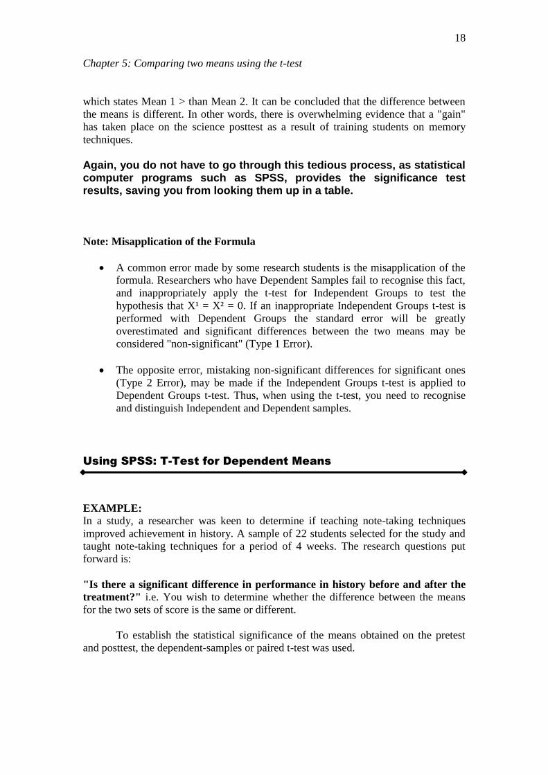
which states Mean 1 > than Mean 2. It can be concluded that the difference between

the means is different. In other words, there is overwhelming evidence that a "gain"

has taken place on the science posttest as a result of training students on memory

techniques.

Again, you do not have to go through this tedious process, as statistical computer programs such as SPSS, provides the significance test results, saving you from looking them up in a table.

Note: Misapplication of the Formula

A common error made by some research students is the misapplication of the

formula. Researchers who have Dependent Samples fail to recognise this fact,

and inappropriately apply the t-test for Independent Groups to test the

hypothesis that X¹ = X² = 0. If an inappropriate Independent Groups t-test is

performed with Dependent Groups the standard error will be greatly

overestimated and significant differences between the two means may be

considered "non-significant" (Type 1 Error).

The opposite error, mistaking non-significant differences for significant ones

(Type 2 Error), may be made if the Independent Groups t-test is applied to

Dependent Groups t-test. Thus, when using the t-test, you need to recognise

and distinguish Independent and Dependent samples.

Using SPSS: T-Test for Dependent Means

EXAMPLE:

In a study, a researcher was keen to determine if teaching note-taking techniques

improved achievement in history. A sample of 22 students selected for the study and

taught note-taking techniques for a period of 4 weeks. The research questions put

forward is:

"Is there a significant difference in performance in history before and after the

treatment?" i.e. You wish to determine whether the difference between the means

for the two sets of score is the same or different.

To establish the statistical significance of the means obtained on the pretest

and posttest, the dependent-samples or paired t-test was used.


19

Data was collected from the same group of subjects on both conditions and

each subject obtains a score on the pretest, and after the treatment (or intervention or

manipulation), a score on the posttest.

Ho: U1 = U2 or Ha: U1 = U2

You will notice that the syntax for the Independent Groups t-test is different from that

of the Dependent groups t-test. In the case of the Independent Groups t-test you have

a grouping variable so you can distinguish between Group 1 and Group 2 whereas

this is not found with the Dependent groups t -test.

The following are the SPSS OUTPUTS: Paired Sample Statistics

HISTORY TEST N Mean Std. Deviation Std. Error Mean

Pair Pretest 40 43.15 12.97 2.05

Posttest 40 63.98 13.16 2.08 The ‘Paired sample statistics’ table above reports that the mean values on the variable

(history test) for the pretest and posttest. The posttest mean is higher (63.98) than the

posttest mean (43.15) indicating improved performance in the history test after the

SPSS PROCEDURES for the dependent groups t-test:

1. Select the Analyze menu.

2. Click on Compare Means and then Paired-Samples T Test ....to open the Paired-Sample T Test dialogue box.

3. Select the test variable(s). [i.e. History Test] and then press the button to move the variables into the Paired Variables: box 4. Click on Continue and then OK.


20

treatment. The standard deviation for the pretest 2.05 and is very close to the standard

deviation for the posttest which is 2.08.

The question remains: Is this mean difference large enough to convince us that there

it is a real significant difference in performance in history a consequence of teaching

note taking techniques)?

Paired Differences

Mean Std . Std. Error t df Sig. (2 tailed) Difference Deviation Mean Lower Upper

Pair Pretest -20.83 15.65 2.47 -25.83 -15.82 -8.43 39 .000 Posttest

t-Value

This "t" value tells you how far away from 0, in terms of the number of standard

errors, the observed difference between the two sample means falls. The "t" value is

obtained by dividing the Mean difference ( - 20.83) by the Std. Error (2.47) which is

equal to – 8.43.

p-value

The p-value shown in the "sig (2 tailed) column is smaller than your chosen alpha

level (0.05) and so you Reject the null hypothesis and argue that there is a real

difference between the pretest and posttest.

In other words, we can conclude, that the observed difference between the two

means is statistically significant.

Mean Difference

This is the difference between the means 43.15 – 63.98 = – 20.83 which students did

significantly better on the posttest.


21

ATTITUDE N Mean Std. Deviation Std. Error Mean

Pair Pretest 22 8.50 3.33 .71

Posttest 22 13.86 2.75 .59

Paired Differences

Mean Std . Std. Error t df Sig.

Deviation Mean Lower Upper (2 tailed)

Pair Pretest -5.36 2.90 .62 -6.65 -4.08 -8.66 21 .000

1 Posttest

LEARNING ACTIVITY

t-Test for Dependent Means or Groups

T-test

Page 3 of 5

CASE STUDY 1: In a study, a researcher was interested in finding out

whether attitude towards science would be enhanced when

students are taught science using the Inquiry Method. A

sample of 22 students were administered an attitude toward

science scale before the experiment. The treatment was

conducted for one semester and after which the same

attitude scale was administered to the same group of

students.


22

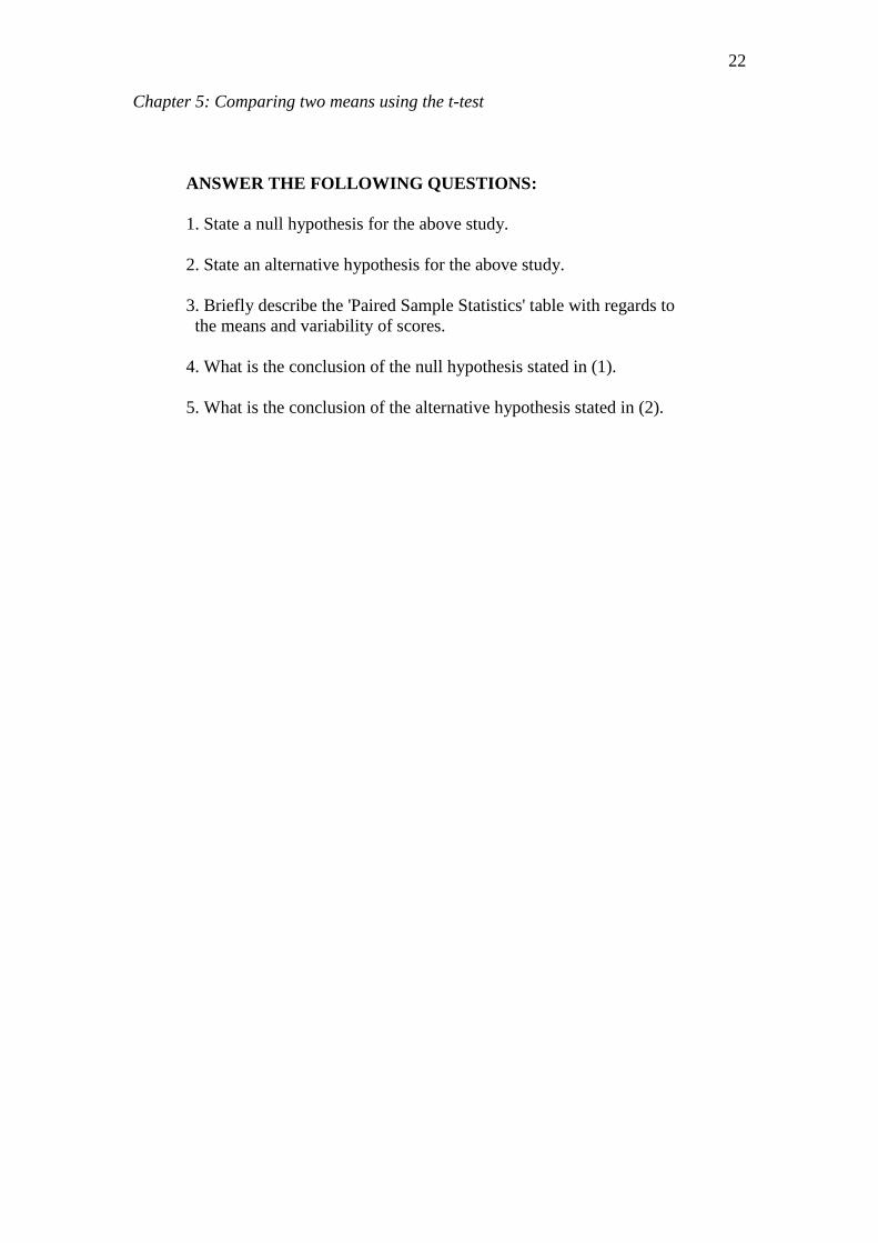
ANSWER THE FOLLOWING QUESTIONS:

1. State a null hypothesis for the above study.

2. State an alternative hypothesis for the above study.

3. Briefly describe the 'Paired Sample Statistics' table with regards to

the means and variability of scores.

4. What is the conclusion of the null hypothesis stated in (1).

5. What is the conclusion of the alternative hypothesis stated in (2).


23

GENDER N Mean Std. Deviation Std. Error Mean

Male 1966 6.9410 2.2858 5.155E-02

Female 2438 6.8351 2.4862 5.035E-02

Levene's Test t-test for for Equality Equality of of Variances Means

F Sig. t df Sig. Mean Std. Error

2-tailed Difference Difference

Equal 19.408 .000 1.456 4402 .145 .1059 7.271E-02

Equal 1.469 4327 .142 .1059 7.206E-02

LEARNING ACTIVITY

t-Test for Independent Means or Groups

T-test

CASE STUDY 2:

A researcher was interested in finding out about the

creative thinking skills of secondary school students. He

administered a 10 item creative thinking to a sample of

4400 sixteen year old students drawn from all over

Malaysia

e 3 of 5


24

ANSWER THE FOLLOWING QUESTIONSE:

1. State a null hypothesis for the above study.

2. State an alternative hypothesis for the above study.

3. Briefly describe the 'Group Statistics' table with regards to

the means and variability of scores.

4. Is there evidence for homogeneity of variance? Explain.

5. What would you do if the significance level is 0.053?

6. What is the conclusion of the null hypothesis stated in (1).

7. What is the conclusion of the alternative hypothesis stated in (2).

SUMMARY

The t-test was developed by a statistician, W.S. Gossett (1878-1937) who

worked in a brewery in Dublin, Ireland.

Researchers are keen to determine whether the differences observed between

two samples represents a real difference between the populations from which

the samples were drawn.

The t-test is a powerful statistic that enables you to determine that the

differences obtained between two groups is statistically significant.

When two groups are INDEPENDENT of each other; it means that the sample

drawn came from two populations. Other words used to mean that the two

groups are independent are "unpaired" groups and "unpooled” groups..

In most educational and social research, the "rule of thumb" is to set the alpha

level at .05. This means that 5% of the time (five times out of a hundred) you

would find a statistically significant difference between the means even if

there is none ("chance").


25

This "t" value tells you how far away from 0, in terms of the number of

standard errors, the observed difference between the two sample means falls.

The Dependent means t-test or the Paired t-test or the Repeated measures t-test

is used when you have data from only one group of subjects. i.e. each subject

obtains two scores under different conditions.

KEY WORDS:

T-test

Independent groups

Dependent groups

Paired groups

t-value

Levene’s test

Critical values

Alpha level

Degress of freedom

One tailed

Two tailed

Null hypothesis

Alternative hypothesis

CHAPTER 4 COMPARING MEANS USING THE...

Documents

Transcript of CHAPTER 4 COMPARING MEANS USING THE...