Chapter 4 · Chapter 4 Decision Trees: Theory and Algorithms Victor E. Lee ... Kent State...

Chapter 4Decision Trees: Theory and Algorithms

Victor E. LeeJohn Carroll UniversityUniversity Heights, [email protected]

Lin LiuKent State UniversityKent, [email protected]

Ruoming JinKent State UniversityKent, [email protected]

4.1 Introduction . . . . . . . . . . . . . . . . . . . . . . . . . . . . . . . . . . . . . . . . . . . . . . . . . . . . . . . . . . . . . . . . . . . . . . 874.2 Top-Down Decision Tree Induction . . . . . . . . . . . . . . . . . . . . . . . . . . . . . . . . . . . . . . . . . . . . . . . . 91

4.2.1 Node Splitting . . . . . . . . . . . . . . . . . . . . . . . . . . . . . . . . . . . . . . . . . . . . . . . . . . . . . . . . . . . . 924.2.2 Tree Pruning . . . . . . . . . . . . . . . . . . . . . . . . . . . . . . . . . . . . . . . . . . . . . . . . . . . . . . . . . . . . . 97

4.3 Case Studies with C4.5 and CART . . . . . . . . . . . . . . . . . . . . . . . . . . . . . . . . . . . . . . . . . . . . . . . . 994.3.1 Splitting Criteria . . . . . . . . . . . . . . . . . . . . . . . . . . . . . . . . . . . . . . . . . . . . . . . . . . . . . . . . . 1004.3.2 Stopping Conditions . . . . . . . . . . . . . . . . . . . . . . . . . . . . . . . . . . . . . . . . . . . . . . . . . . . . . . 1004.3.3 Pruning Strategy . . . . . . . . . . . . . . . . . . . . . . . . . . . . . . . . . . . . . . . . . . . . . . . . . . . . . . . . . 1014.3.4 Handling Unknown Values: Induction and Prediction . . . . . . . . . . . . . . . . . . . . . . 1014.3.5 Other Issues: Windowing and Multivariate Criteria . . . . . . . . . . . . . . . . . . . . . . . . 102

4.4 Scalable Decision Tree Construction . . . . . . . . . . . . . . . . . . . . . . . . . . . . . . . . . . . . . . . . . . . . . . . 1034.4.1 RainForest-Based Approach . . . . . . . . . . . . . . . . . . . . . . . . . . . . . . . . . . . . . . . . . . . . . . 1044.4.2 SPIES Approach . . . . . . . . . . . . . . . . . . . . . . . . . . . . . . . . . . . . . . . . . . . . . . . . . . . . . . . . . 1054.4.3 Parallel Decision Tree Construction . . . . . . . . . . . . . . . . . . . . . . . . . . . . . . . . . . . . . . . 107

4.5 Incremental Decision Tree Induction . . . . . . . . . . . . . . . . . . . . . . . . . . . . . . . . . . . . . . . . . . . . . . 1084.5.1 ID3 Family . . . . . . . . . . . . . . . . . . . . . . . . . . . . . . . . . . . . . . . . . . . . . . . . . . . . . . . . . . . . . . . 1084.5.2 VFDT Family . . . . . . . . . . . . . . . . . . . . . . . . . . . . . . . . . . . . . . . . . . . . . . . . . . . . . . . . . . . . 1104.5.3 Ensemble Method for Streaming Data . . . . . . . . . . . . . . . . . . . . . . . . . . . . . . . . . . . . . 113

4.6 Summary . . . . . . . . . . . . . . . . . . . . . . . . . . . . . . . . . . . . . . . . . . . . . . . . . . . . . . . . . . . . . . . . . . . . . . . . . 114Bibliography . . . . . . . . . . . . . . . . . . . . . . . . . . . . . . . . . . . . . . . . . . . . . . . . . . . . . . . . . . . . . . . . . . . . . 115

4.1 IntroductionOne of the most intuitive tools for data classification is the decision tree. It hierarchically par-

titions the input space until it reaches a subspace associated with a class label. Decision trees areappreciated for being easy to interpret and easy to use. They are enthusiastically used in a range of

87

Copyrighted Material - Taylor and Francis

88 Data Classification: Algorithms and Applications

business, scientific, and health care applications [12,15,71] because they provide an intuitive meansof solving complex decision-making tasks. For example, in business, decision trees are used foreverything from codifying how employees should deal with customer needs to making high-valueinvestments. In medicine, decision trees are used for diagnosing illnesses and making treatmentdecisions for individuals or for communities.

A decision tree is a rooted, directed tree akin to a flowchart. Each internal node correspondsto a partitioning decision, and each leaf node is mapped to a class label prediction. To classify adata item, we imagine the data item to be traversing the tree, beginning at the root. Each internalnode is programmed with a splitting rule, which partitions the domain of one (or more) of the data’sattributes. Based on the splitting rule, the data item is sent forward to one of the node’s children.This testing and forwarding is repeated until the data item reaches a leaf node.

Decision trees are nonparametric in the statistical sense: they are not modeled on a probabil-ity distribution for which parameters must be learned. Moreover, decision tree induction is almostalways nonparametric in the algorithmic sense: there are no weight parameters which affect theresults.

Each directed edge of the tree can be translated to a Boolean expression (e.g., x1 > 5); therefore,a decision tree can easily be converted to a set of production rules. Each path from root to leafgenerates one rule as follows: form the conjunction (logical AND) of all the decisions from parentto child.

Decision trees can be used with both numerical (ordered) and categorical (unordered) attributes.There are also techniques to deal with missing or uncertain values. Typically, the decision rules areunivariate. That is, each partitioning rule considers a single attribute. Multivariate decision ruleshave also been studied [8,9]. They sometimes yield better results, but the added complexity is oftennot justified. Many decision trees are binary, with each partitioning rule dividing its subspace intotwo parts. Even binary trees can be used to choose among several class labels. Multiway splitsare also common, but if the partitioning is into more than a handful of subdivisions, then both theinterpretability and the stability of the tree suffers. Regression trees are a generalization of decisiontrees, where the output is a real value over a continuous range, instead of a categorical value. Forthe remainder of the chapter, we will assume binary, univariate trees, unless otherwise stated.

Table 4.1 shows a set of training data to answer the classification question, “What sort of contactlenses are suitable for the patient?” This data was derived from a public dataset available from theUCI Machine Learning Repository [3]. In the original data, the age attribute was categorical withthree age groups. We have modified it to be a numerical attribute with age in years. The next threeattributes are binary-valued. The last attribute is the class label. It is shown with three values (lensestypes): {hard, soft, no}. Some decision tree methods support only binary decisions. In this case, wecan combine hard and soft to be simply yes.

Next, we show four different decision trees, all induced from the same data. Figure 4.1(a) showsthe tree generated by using the Gini index [8] to select split rules when the classifier is targetingall three class values. This tree classifies the training data exactly, with no errors. In the leaf nodes,the number in parentheses indicates how many records from the training dataset were classified intothis bin. Some leaf nodes indicate a single data item. In real applications, it may be unwise to permitthe tree to branch based on a single training item because we expect the data to have some noiseor uncertainty. Figure 4.1(b) is the result of pruning the previous tree, in order to achieve a smallertree while maintaining nearly the same classification accuracy. Some leaf nodes now have a pair ofnumber: (record count, classification errors).

Figure 4.2(a) shows a 2-class classifier (yes, no) and uses the C4.5 algorithm for selecting thesplits [66]. A very aggressively pruned tree is shown in Figure 4.2(b). It misclassifies 3 out of 24training records.


Decision Trees: Theory and Algorithms 89

TABLE 4.1: Example: Contact Lens Recommendations

Age Near-/Far-sightedness Astigmatic Tears Contacts Recommended13 nearsighted no reduced no18 nearsighted no normal soft14 nearsighted yes reduced no16 nearsighted yes normal hard11 farsighted no reduced no18 farsighted no normal soft8 farsighted yes reduced no8 farsighted yes normal hard

26 nearsighted no reduced no35 nearsighted no normal soft39 nearsighted yes reduced no23 nearsighted yes normal hard23 farsighted no reduced no36 farsighted no normal soft35 farsighted yes reduced no32 farsighted yes normal no55 nearsighted no reduced no64 nearsighted no normal no63 nearsighted yes reduced no51 nearsighted yes normal hard47 farsighted no reduced no44 farsighted no normal soft52 farsighted yes reduced no46 farsighted yes normal no

(a) CART algorithm (b) Pruned version

FIGURE 4.1 (See color insert.): 3-class decision trees for contact lenses recommendation.



(a) C4.5 algorithm (b) Pruned version

FIGURE 4.2 (See color insert.): 2-class decision trees for contact lenses recommendation.

Optimality and ComplexityConstructing a decision tree that correctly classifies a consistent1 data set is not difficult. Our prob-lem, then, is to construct an optimal tree, but what does optimal mean? Ideally, we would like amethod with fast tree construction, fast predictions (shallow tree depth), accurate predictions, androbustness with respect to noise, missing values, or concept drift. Should it treat all errors the same,or it is more important to avoid certain types of false positives or false negatives? For example, ifthis were a medical diagnostic test, it may be better for a screening test to incorrectly predict that afew individuals have an illness than to incorrectly decide that some other individuals are healthy.

Regardless of the chosen measure of goodness, finding a globally optimal result is not feasiblefor large data sets. The number of possible trees grows exponentially with the number of attributesand with the number of distinct values for each attribute. For example, if one path in the tree fromroot to leaf tests d attributes, there are d! different ways to order the tests. Hyafil and Rivest [35]proved that constructing a binary decision tree that correctly classifies a set of N data items suchthat the expected number of steps to classify an item is minimal is NP-complete. Even for moreesoteric schemes, namely randomized decision trees and quantum decision trees, the complexity isstill NP-complete [10].

In most real applications, however, we know we cannot make a perfect predictor anyway (dueto unknown differences between training data and test data, noise and missing values, and conceptdrift over time). Instead, we favor a tree that is efficient to construct and/or update and that matchesthe training set “well enough.”

Notation We will use the following notation (further summarized for data and partition in Table4.2) to describe the data, its attributes, the class labels, and the tree structure. A data item x isa vector of d attribute values with an optional class label y. We denote the set of attributes as A ={A1,A2, . . . ,Ad}. Thus, we can characterize x as {x1,x2, . . . ,xd}, where x1 ∈A1,x2 ∈ A2, . . . ,xd ∈Ad .Let Y = {y1,y2, . . . ,ym} be the set of class labels. Each training item x is mapped to a class value ywhere y ∈ Y. Together they constitute a data tuple 〈x,y〉. The complete set of training data is X.

1A training set is inconsistent if two items have different class values but are identical in all other attribute values.



TABLE 4.2: Summary of Notation for Data and Partitions

Symbol DefinitionX set of all training data = {x1, . . . ,xn}A set of attributes = {A1, . . . ,Ad}Y domain of class values = {y1, . . . ,ym}Xi a subset of XS a splitting rule

XS a partitioning of X into {X1, . . . ,Xk}

A partitioning rule S subdivides data set X into a set of subsets collectively known as XS; that is,XS = {X1,X2, . . . ,Xk} where

⋃i Xi = X. A decision tree is a rooted tree in which each set of children

of each parent node corresponds to a partitioning (XS) of the parent’s data set, with the full data setassociated with the root. The number of items in Xi that belong to class y j is |Xi j|. The probability

that a randomly selected member of Xi is of class y j is pi j =|Xi j ||Xi| .

The remainder of the chapter is organized as follows. Section 4.2 describes the operation ofclassical top-down decision tree induction. We break the task down into several subtasks, examin-ing and comparing specific splitting and pruning algorithms that have been proposed. Section 4.3features case studies of two influential decision tree algorithms, C4.5 [66] and CART [8]. Here wedelve into the details of start-to-finish decision tree induction and prediction. In Section 4.4, wedescribe how data summarization and parallelism can be used to achieve scalability with very largedatasets. Then, in Section 4.5, we introduce techniques and algorithms that enable incremental treeinduction, especially in the case of streaming data. We conclude with a review of the advantagesand disadvantages of decision trees compared to other classification methods.

4.2 Top-Down Decision Tree InductionThe process of learning the structure of a decision tree, to construct the classifier, is called deci-

sion tree induction [63]. We first describe the classical approach, top-down selection of partitioningrules on a static dataset. We introduce a high-level generic algorithm to convey the basic idea, andthen look deeper at various steps and subfunctions within the algorithm.

The decision tree concept and algorithm can be tracked back to two independent sources: AID(Morgan and Sonquist, 1963) [56] and CLS in Experiments in Induction (Hunt, Marin, and Stone,1966) [34]. The algorithm can be written almost entirely as a single recursive function, as shownin Algorithm 4.1. Given a set of data items, which are each described by their attribute values, thefunction builds and returns a subtree. The key subfunctions are shown in small capital letters. First,the function checks if it should stop further refinement of this branch of the decision tree (line 3,subfunction STOP). If so, it returns a leaf node, labeled with the class that occurs most frequentlyin the current data subset X ′. Otherwise, it procedes to try all feasible splitting options and selectsthe best one (line 6, FINDBESTSPLITTINGRULE). A splitting rule partitions the dataset into subsets.What constitutes the “best” rule is perhaps the most distinctive aspect of one tree induction algorithmversus another. The algorithm creates a tree node for the chosen rule (line 8).

If a splitting rule draws all the classification information out of its attribute, then the attributeis exhausted and is ineligible to be used for splitting in any subtree (lines 9–11). For example, if adiscrete attribute with k different values is used to create k subsets, then the attribute is “exhausted.”



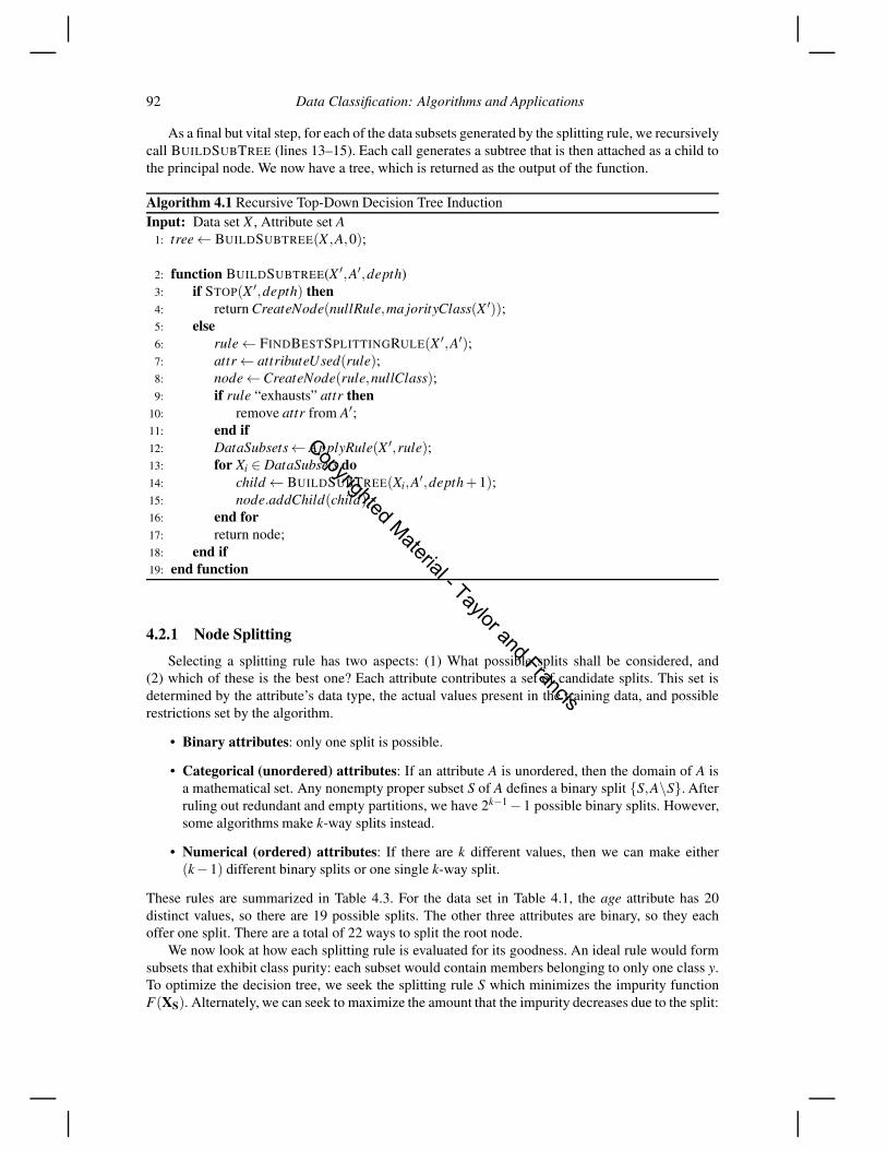
As a final but vital step, for each of the data subsets generated by the splitting rule, we recursivelycall BUILDSUBTREE (lines 13–15). Each call generates a subtree that is then attached as a child tothe principal node. We now have a tree, which is returned as the output of the function.

Algorithm 4.1 Recursive Top-Down Decision Tree InductionInput: Data set X , Attribute set A

1: tree← BUILDSUBTREE(X ,A,0);

2: function BUILDSUBTREE(X ′,A′,depth)3: if STOP(X ′,depth) then4: return CreateNode(nullRule,ma jorityClass(X ′));5: else6: rule← FINDBESTSPLITTINGRULE(X ′,A′);7: attr← attributeUsed(rule);8: node←CreateNode(rule,nullClass);9: if rule “exhausts” attr then

10: remove attr from A′;11: end if12: DataSubsets← ApplyRule(X ′,rule);13: for Xi ∈ DataSubsets do14: child ← BUILDSUBTREE(Xi,A′,depth+1);15: node.addChild(child);16: end for17: return node;18: end if19: end function

4.2.1 Node Splitting

Selecting a splitting rule has two aspects: (1) What possible splits shall be considered, and(2) which of these is the best one? Each attribute contributes a set of candidate splits. This set isdetermined by the attribute’s data type, the actual values present in the training data, and possiblerestrictions set by the algorithm.

• Binary attributes: only one split is possible.

• Categorical (unordered) attributes: If an attribute A is unordered, then the domain of A isa mathematical set. Any nonempty proper subset S of A defines a binary split {S,A\S}. Afterruling out redundant and empty partitions, we have 2k−1−1 possible binary splits. However,some algorithms make k-way splits instead.

• Numerical (ordered) attributes: If there are k different values, then we can make either(k− 1) different binary splits or one single k-way split.

These rules are summarized in Table 4.3. For the data set in Table 4.1, the age attribute has 20distinct values, so there are 19 possible splits. The other three attributes are binary, so they eachoffer one split. There are a total of 22 ways to split the root node.

We now look at how each splitting rule is evaluated for its goodness. An ideal rule would formsubsets that exhibit class purity: each subset would contain members belonging to only one class y.To optimize the decision tree, we seek the splitting rule S which minimizes the impurity functionF(XS). Alternately, we can seek to maximize the amount that the impurity decreases due to the split:



TABLE 4.3: Number of Possible Splits Based on Attribute Type

Attribute Type Binary Split Multiway SplitBinary 1 1 (same as binary)

Categorical (unordered) 2k−22 = 2k−1−1 one k-way split

Numerical (ordered) k−1 one k-way split

ΔF(S) = F(X)−F(XS). The authors of CART [8] provide an axiomatic definition of an impurityfunction F :

Definition 4.1 An impurity function F for a m-state discrete variable Y is a function defined on theset of all m-tuple discrete probability vectors (p1, p2, . . . , pm) such that

1. F is maximum only at ( 1m ,

1m , . . . ,

1m),

2. F is minimum only at the “purity points” (1,0, . . . ,0),(0,1, . . . ,0), . . . ,(0,0, . . . ,1),

3. F is symmetric with respect to p1, p2, . . . , pm.

We now consider several basic impurity functions that meet this definition.

1. Error RateA simple measure is the percentage of misclassified items. If y j is the class value that appears

most frequently in partition Xi, then the error rate for Xi is E(Xi) =|{y=y j :(x,y)∈Xi}|

|Xi| = 1− pi j.The error rate for the entire split XS is the weighted sum of the error rates for each subset.This equals the total number of misclassifications, normalized by the size of X.

ΔFerror(S) = E(X)−∑i∈S

|Xi||X |E(Xi). (4.1)

This measure does not have good discriminating power. Suppose we have a two-class system,in which y is the majority class not only in X , but in every available partitioning of X . Errorrate will consider all such partitions equal in preference.

2. Entropy and Information Gain (ID3)Quinlan’s first decision tree algorithm, ID3 [62], uses information gain, or equivalently, en-

tropy loss, as the goodness function for dataset partitions. In his seminal work on informationtheory, Shannnon [70] defined information entropy as the degree of uncertainty of a (discrete)random variable Y , formulated as

HX (Y ) =−∑y∈Y

py log py (4.2)

where py is the probability that a random selection would have state y. We add a subscript(e.g., X ) when it is necessary to indicate the dataset being measured. Information entropy canbe interpreted at the expected amount of information, measured in bits, needed to describe thestate of a system. Pure systems require the least information. If all objects in the system arein the same state k, then pk = 1, log pk = 0, so entropy H = 0. There is no randomness in thesystem; no additional classification information is needed. At the other extreme is maximaluncertainty, when there are an equal number of objects in each of the |Y | states, so py =

1|Y | ,

for all y. Then, H(Y ) = −|Y |( 1|Y | log 1

|Y | ) = log |Y |. To describe the system we have to fullyspecify all the possible states using log |Y | bits. If the system is pre-partitioned into subsets



according to another variable (or splitting rule) S, then the information entropy of the overallsystem is the weighted sum of the entropies for each partition, HXi(Y ). This is equivalent tothe conditional entropy HX(Y |S).

ΔFin f oGain(S) =−∑y∈Y

py log py +∑i∈S

|Xi||X | ∑y∈Y

piy log piy (4.3)

=HX(Y ) −∑i∈S

piHXi(Y )

=HX(Y ) −HX(Y |S).

We know limp→0 p log p goes to 0, so if a particular class value y is not represented in adataset, then it does not contribute to the system’s entropy.

A shortcoming of the information gain criterion is that it is biased towards splits with largerk. Given a candidate split, if subdividing any subset provides additional class differentiation,then the information gain score will always be better. That is, there is no cost to making asplit. In practice, making splits into many small subsets increases the sensitivity to individualtraining data items, leading to overfit. If the split’s cardinality k is greater than the number ofclass values m, then we might be “overclassifying” the data.

For example, suppose we want to decide whether conditions are suitable for holding a sem-inar, and one of the attributes is day of the week. The “correct” answer is Monday throughFriday are candidates for a seminar, while Saturday and Sunday are not. This is naturally abinary split, but ID3 would select a 7-way split.

3. Gini Criterion (CART)Another influential and popular decision tree program, CART [8], uses the Gini index for asplitting criterion. This can be interpreted as the expected error if each individual item wererandomly classified according to the probability distribution of class membership within eachsubset. Like ID3, the Gini index is biased towards splits with larger k.

Gini(Xi) = ∑y∈Y

piy(1− piy) = 1−∑y∈Y

p2iy (4.4)

ΔFGini(S) = Gini(X)−∑i∈S

|Xi||X |Gini(Xi). (4.5)

4. Normalized Measures — Gain Ratio (C4.5)To remedy ID3’s bias towards higher k splits, Quinlan normalized the information gain tocreate a new measure called gain ratio [63]. Gain ratio is featured in Quinlan’s well-knowndecision tree tool, C4.5 [66].

splitIn f o(S) =−∑i∈S

|Xi||X | log

|Xi||X | = H(S) (4.6)

ΔFgainRatio(S) =ΔFin f oGain(S)splitIn f o(S)

=H(Y )−H(Y |S)

H(S). (4.7)

SplitInfo considers only the number of subdivisions and their relative sizes, not their purity. Itis higher when there are more subdivisions and when they are more balanced in size. In fact,splitInfo is the entropy of the split where S is the random variable of interest, not Y . Thus, the



gain ratio seeks to factor out the information gained from the type of partitioning as opposedto what classes were contained in the partitions.

The gain ratio still has a drawback. A very imbalanced partitioning will yield a low value forH(S) and thus a high value for ΔFgainRatio, even if the information gain is not very good. Toovercome this, C4.5 only considers splits whose information gain scores are better than theaverage value [66].

5. Normalized Measures — Information DistanceLopez de Mantaras has proposed using normalized information distance as a splitting crite-rion [51]. The distance between a target attribute Y and a splitting rule S is the sum of the twoconditional entropies, which is then normalized by dividing by their joint entropy:

dN(Y,S) =H(Y |S)+H(S|Y)

H(Y,S)(4.8)

=

∑i∈S

pi ∑y∈Y

piy log piy + ∑y∈Y

pi ∑i∈S

pyi log pyi

∑i∈S

∑y∈Y

piy log piy.

This function is a distance metric; that is, it meets the nonnegative, symmetry, and triangleinequality properties, and dN(Y,S) = 0 when Y = S. Moreover its range is normalized to [0,1].Due to its construction, it solves both the high-k bias and the imbalanced partition problemsof information gain (ID3) and gain ratio (C4.5).

6. DKM Criterion for Binary ClassesIn cases where the class attribute is binary, the DKM splitting criterion, named after Diet-terich, Kearns, and Mansour [17, 43] offers some advantages. The authors have proven thatfor a given level of prediction accuracy, the expected size of a DKM-based tree is smaller thanfor those constructed using C4.5 or Gini.

DKM(Xi) = 2√

pi(1− pi) (4.9)

ΔFDKM(S) = DKM(X)−∑i∈S

|Xi||X |DKM(Xi).

7. Binary Splitting CriteriaBinary decision trees as often used, for a variety of reasons. Many attributes are naturallybinary, binary trees are easy to interpret, and binary architecture avails itself of additionalmathematical properties. Below are a few splitting criteria especially for binary splits. Thetwo partitions are designated 0 and 1.

(a) Twoing CriterionThis criterion is presented in CART [8] as an alternative to the Gini index. Its valuecoincides with the Gini index value for two-way splits.

ΔFtwoing(S) =p0 · p1

4(∑

y∈Y|py0− py1|)2. (4.10)

(b) Orthogonality MeasureFayyad and Irani measure the cosine angle between the class probability vectors fromthe two partitions [22]. (Recall the use of probability vectors in Definition 4.1 for animpurity function.) If the split puts all instances of a given class in one partition but



not the other, then the two vectors are orthogonal, and the cosine is 0. The measure isformulated as (1− cosθ) so that we seek a maximum value.

ORT (S) = 1− cos(P0,P1) = 1−∑

y∈Ypy0 py1

||P0|| · ||P1||. (4.11)

(c) Other Vector Distance MeasuresOnce we see that a vector representation and cosine distance can be used, many otherdistance or divergence criteria come to mind, such as Jensen-Shannon divergence [75],Kolmogorov-Smirmov distance [24], and Hellinger distance [13].

8. Minimum Description LengthQuinlan and Rivest [65] use the Minimum Description Length (MDL) approach to simulta-neous work towards the best splits and the most compact tree. A description of a solutionconsists of an encoded classification model (tree) plus discrepancies between the model andthe actual data (misclassifications). To find the minimum description, we must find the bestbalance between a small tree with relatively high errors and a more expansive tree with littleor no misclassifications. Improved algorithms are offered in [83] and [82].

9. Comparing Splitting CriteriaWhen a new splitting criterion is introduced, it is compared to others for tree size and accu-racy, and sometimes for robustness, training time, or performance with specific types of data.The baselines for comparison are often C4.5(Gain ratio), CART(Gini), and sometimes DKM.For example, Shannon entropy is compared to Renyi and Tsallis entropies in [50]. While onemight not be too concerned about tree size, perhaps because one does not have a large numberof attributes, a smaller (but equally accurate) tree implies that each decision is accomplishingmore classification work. In that sense, a smaller tree is a better tree.

In 1999, Lim and Loh compared 22 decision tree, nine statistical, and two neural networkalgorithms [49]. A key result was that there was no statistically significant difference in clas-sification accuracy among the top 21 algorithms. However, there were large differences intraining time. The most accurate algorithm, POLYCAST, required hours while similarly ac-curate algorithms took seconds. It is also good to remember that if high quality training dataare not available, then algorithms do not have the opportunity to perform at their best. Thebest strategy may be to pick a fast, robust, and competitively accurate algorithm. In Lim andLoh’s tests, C4.5 and an implementation of CART were among the best in terms of balancedspeed and accuracy.

Weighted error penaltiesAll of the above criteria have assumed that all errors have equal significance. However, for manyappliations this is not the case. For a binary classifier (class is either Yes or No), there are fourpossible prediction results, two correct results and two errors:

1. Actual class = Yes; Predicted class = Yes: True Positive

2. Actual class = Yes; Predicted class = No: False Negative

3. Actual class = No; Predicted class = Yes: False Positive

4. Actual class = No; Predicted class = No: True Negative

If there are k different class values, then there are k(k−1) different types of errors. We can assigneach type of error a weight and then modify the split goodness criterion to include these weights.For example, a binary classifier could have wFP and wFN for False Positive and False Negative,



respectively. More generally, we can say the weight is wp,t , where p is the predicted class and t isthe true class. wtt = 0 because this represents a correct classification, hence no error.

Let us look at a few examples of weights being incorporated into an impurity function. Let Ti bethe class predicted for partition Xi, which would be the most populous class value in Xi.

Weighted Error Rate: Instead of simply counting all the misclassifications, we count how manyof each type of classification occurs, multiplied by its weight.

Ferror,wt =∑i∈S∑y∈Y wTi ,y|Xiy|

|X | =∑i∈S∑y∈Y

wTi,y piy. (4.12)

Weighted Entropy: The modified entropy can be incorporated into the information gain, gainratio, or information distance criterion.

H(Y )wt =−∑y∈Y

wTi ,y py log py. (4.13)

4.2.2 Tree Pruning

Using the splitting rules presented above, the recursive decision tree induction procedure willkeep splitting nodes as long as the goodness function indicates some improvement. However, thisgreedy strategy can lead to overfitting, a phenomenon where a more precise model decreases theerror rate for the training dataset but increases the error rate for the testing dataset. Additionally, alarge tree might offer only a slight accuracy improvement over a smaller tree. Overfit and tree sizecan be reduced by pruning, replacing subtrees with leaf nodes or simpler subtrees that have the sameor nearly the same classification accuracy as the unpruned tree. As Breiman et al. have observed,pruning algorithms affect the final tree much more than the splitting rule.

Pruning is basically tree growth in reverse. However, the splitting criteria must be different thanwhat was used during the growth phase; otherwise, the criteria would indicate that no pruning isneeded. Mingers (1989) [55] lists five different pruning algorithms. Most of them require using adifferent data sample for pruning than for the initial tree growth, and most of them introduce a newimpurity function. We describe each of them below.

1. Cost Complexity Pruning, also called Error Complexity Pruning (CART) [8]This multi-step pruning process aims to replace subtrees with a single node. First, we definea cost-benefit ratio for a subtree: the number of misclassification errors it removes divided bythe number of leaf nodes it adds. If LX is the set of leaf node data subsets of X , then

error complexity =E(X)−∑Li∈LX E(Li)

|LX |− 1. (4.14)

Compute error complexity for each internal node, and convert the one with the smallest value(least increase in error per leaf) to a leaf node. Recompute values and repeat pruning until onlythe root remains, but save each intermediate tree. Now, compute new (estimated) error ratesfor every pruned tree, using a new test dataset, different than the original training set. Let T0be the pruned tree with the lowest error rate. For the final selection, pick the smallest tree T ′whose error rate is within one standard error of T0’s error rate, where standard error is defined

as SE =

√E(T0)(1−E(T0))

N .

For example, in Figure 4.2(a), the [age> 55?] decision node receives 6 training items: 5 itemshave age ≤ 55, and 1 item has age > 55. The subtree has no misclassification errors and 2leaves. If we replace the subtree with a single node, it will have an error rate of 1/6. Thus,error complexity(age55) = 1/6−0

2−1 = 0.167. This is better than the [age > 18?] node, whichhas an error complexity of 0.333.



2. Critical Value Pruning [54]This pruning strategy follows the same progressive pruning approach as cost-complexitypruning, but rather than defining a new goodness measure just for pruning, it reuses the samecriterion that was used for tree growth. It records the splitting criteria values for each nodeduring the growth phase. After tree growth is finished, it goes back in search of interior nodeswhose splitting criteria values fall below some threshold. If all the splitting criteria valuesin a node’s subtree are also below the threshold, then the subtree is replaced with a singleleaf node. However, due to the difficulty of selecting the right threshold value, the practicalapproach is to prune the weakest subtree, remember this pruned tree, prune the next weakestsubtree, remember the new tree, and so on, until only the root remains. Finally, among theseseveral pruned trees, the one with the lowest error rate is selected.

3. Minimum Error Pruning [58]The error rate defined in Equation 4.1 is the actual error rate for the sample (training) data.Assuming that all classes are in fact equally likely, Niblett and Bratko [58] prove that theexpected error rate is

E ′(Xi) =|Xi| ·E(Xi)+m−1

|Xi|+m, (4.15)

where m is the number of different classes. Using this as an impurity criterion, this pruningmethod works just like the tree growth step, except it merges instead of splits. Starting fromthe parent of a leaf node, it compares its expected error rate with the size-weighted sum of theerror rates of its children. If the parent has a lower expected error rate, the subtree is convertedto a leaf. The process is repeated for all parents of leaves until the tree has been optimized.Mingers [54] notes a few flaws with this approach: 1) the assumption of equally likely classesis unreasonable, and 2) the number of classes strongly affects the degree of pruning.

Looking at the [age > 55?] node in Figure 4.2(a) again, the current subtree has a scoreE ′(subtree) = (5/6) 5(0)+2−1

5+2 + (1/6) 1(0)+2−11+2 = (5/6)(1/7)+ (1/6)(1/3) = 0.175. If we

change the node to a leaf, we get E ′(lea f ) = 6(1/6)+2−16+2 = 2/8 = 0.250. The pruned ver-

sion has a higher expected error, so the subtree is not pruned.

4. Reduced Error Pruning (ID3) [64]This method uses the same goodness criteria for both tree growth and pruning, but uses dif-ferent data samples for the two phases. Before the initial tree induction, the training dataset isdivided into a growth dataset and a pruning dataset. Initial tree induction is performed usingthe growth dataset. Then, just as in minimum error pruning, we work bottom-to-top, but thistime the pruning dataset is used. We retest each parent of children to see if the split is stilladvantageous, when a different data sample is used. One weakness of this method is that itrequires a larger quantity of training data. Furthermore, using the same criteria for growingand pruning will tend to under-prune.

5. Pessimistic Error Pruning (ID3, C4.5) [63, 66]This method eliminates the need for a second dataset by estimating the training set bias andcompensating for it. A modified error function is created (as in minimum error pruning),which is used for bottom-up retesting of splits. In Quinlan’s original version, the adjustederror is estimated to be 1

2 per leaf in a subtree. Given tree node v, let T (v) be the subtree



rooted at v, and L(v) be the leaf nodes under v. Then,

not pruned: Epess(T (v)) = ∑l∈L(v)

E(l)+|L(v)|

2(4.16)

if pruned: Epess(v) = E(v)+12.

(4.17)

Because this adjustment alone might still be too optimistic, the actual rule is that a subtreewill be pruned if the decrease in error is larger than the Standard Error.

In C4.5, Quinlan modified pessimistic error pruning to be more pessimistic. The new esti-mated error is the upper bound of the binomial distribution confidence interval, UCF(E , |Xi|).C4.5 uses 25% confidence by default. Note that the binomial distribution should not be ap-proximated by the normal distribution, because the approximation is not good for small errorrates.

For our [age > 55?] example in Figure 4.2(a), C4.5 would assign the subtree an error score of(5/6)UCF(0,5)+ (1/6)UCF(0,1) = (0.833)0.242+(0.166).750= 0.327. If we prune, thenthe new root has a score of UCF(1,6) = 0.390. The original split has a better error score, sowe retain the split.

6. Additional Pruning MethodsMansour [52] has computed a different upper bound for pessimistic error pruning, based onthe Chernoff bound. The formula is simpler than Quinlan’s but requires setting two param-eters. Kearns and Mansour [44] describe an algorithm with good theoretical guarantees fornear- optimal tree size. Mehta et al. present an MDL-based method that offers a better com-bination of tree size and speed than C4.5 or CART on their test data.

Esposito et al. [20] have compared the five earlier pruning techniques. They find that cost-complexity pruning and reduced error pruning tend to overprune, i.e., create smaller but less accuratedecision trees. Other methods (error-based pruning, pessimistic error pruning, and minimum errorpruning) tend to underprune. However, no method clearly outperforms others on all measures. Thewisest strategy for the user seems to be to try several methods, in order to have a choice.

4.3 Case Studies with C4.5 and CARTTo illustrate how a complete decision tree classifier works, we look at the two most prominent

algorithms: CART and C4.5. Interestingly, both are listed among the top 10 algorithms in all of datamining, as chosen at the 2006 International Conference on Data Mining [85].

CART was developed by Breiman, Friedman, Olshen, and Stone, as a research work. The deci-sion tree induction problem and their solution is described in detail in their 1984 book, Classificationand Regression Trees [8]. C4.5 gradually evolved out of ID3 during the late 1980s and early 1990s.Both were developed by J. Ross Quinlan. Early on C4.5 was put to industrial use, so there has been asteady stream of enhancements and added features. We focus on the version described in Quinlan’s1993 book, C4.5: Programs for Machine Learning [66].



4.3.1 Splitting Criteria

CART: CART was designed to construct binary trees only. It introduced both the Gini and twoingcriteria. Numerical attributes are first sorted, and then the k−1 midpoints between adjacent numer-ical values are used as candidate split points. Categorical attributes with large domains must try all2k−1−1 possible binary splits. To avoid excessive computation, the authors recommend not havinga large number of different categories.

C4.5: In default mode, C4.5 makes binary splits for numerical attributes and k-way splits for cate-gorical attributes. ID3 used the Information Gain criterion. C4.5 normally uses the Gain Ratio, withthe caveat that the chosen splitting rule must also have an Information Gain that is stronger thanthe average Information Gain. Numerical attributes are first sorted. However, instead of selectingthe midpoints, C4.5 considers each of the values themselves as the split points. If the sorted valuesare (x1,x2, . . . ,xn), then the candidate rules are {x > x1,x > x2, . . . ,x > xn−1}. Optionally, insteadof splitting categorical attributes into k branches, one branch for each different attribute value, theycan be split into b branches, where b is a user-designated number. To implement this, C4.5 first per-forms the k-way split and then greedily merges the most similar children until there are b childrenremaining.

4.3.2 Stopping Conditions

In top-down tree induction, each split produces new nodes that recursively become the startingpoints for new splits. Splitting continues as long as it is possible to continue and to achieve a netimprovement, as measured by the particular algorithm. Any algorithm will naturally stop trying tosplit a node when either the node achieves class purity or the node contain only a single item. Thenode is then designated a leaf node, and the algorithm chooses a class label for it.

However, stopping only under these absolute conditions tends to form very large trees that areoverfit to the training data. Therefore, additional stopping conditions that apply pre-pruning maybe used. Below are several possible conditions. Each is independent of the other and employs somethreshold parameter.

• Data set size reaches a minimum.

• Splitting the data set would make children that are below the minimize size.

• Splitting criteria improvement is too small.

• Tree depth reaches a maximum.

• Number of nodes reaches a maximum.

CART: Earlier, the authors experimented with a minimum improvement rule: |ΔFGini| > β. How-ever, this was abandoned because there was no right value for β. While the immediate benefit ofsplitting a node may be small, the cumulative benefit from multiple levels of splitting might besubstantial. In fact, even if splitting the current node offers only a small reduction of impurity, itschidren could offer a much larger reduction. Consequently, CART’s only stopping condition is aminimum node size. Instead, it strives to perform high-quality pruning.

C4.5: In ID3, a Chi-squared test was used as a stopping condition. Seeing that this sometimes causedoverpruning, Quinlan removed this stopping condition in C4.5. Like CART, the tree is allowed togrow unfettered, with only one size constraint: any split must have at least two children containingat least nmin training items each, where nmin defaults to 2.



4.3.3 Pruning Strategy

CART uses cost complexity pruning. This is one of the most theoretically sound pruning methods.To remove data and algorithmic bias from the tree growth phase, it uses a different goodness cri-terion and a different dataset for pruning. Acknowledging that there is still statistical uncertaintyabout the computations, a standard error statistic is computed, and the smallest tree that is with theerror range is chosen.

C4.5 uses pessimistic error pruning with the binomial confidence interval. Quinlan himself acknowl-edges that C4.5 may be applying statistical concepts loosely [66]. As a heuristic method, however,it works about as well as any other method. Its major advantage is that it does not require a separatedataset for pruning. Moreover, it allows a subtree to be replaced not only by a single node but alsoby the most commonly selected child.

4.3.4 Handling Unknown Values: Induction and Prediction

One real-world complication is that some data items have missing attribute values. Using thenotation x = {x1,x2, . . . ,xd}, some of the xi values may be missing (null). Missing values generatethree concerns:

1. Choosing the Best Split: If a candidate splitting criterion uses attribute Ai but some items haveno values for Ai, how should we account for this? How do we select the best criteria, whenthey have different proportions of missing values?

2. Partitioning the Training Set: Once a splitting criteria is selected, to which child node will theimcomplete data items be assigned?

3. Making Predictions: If making class predictions for items with missing attribute values, howwill they proceed down the tree?

Recent studies have compared different techniques for handling missing values in decision trees [18,67]. CART and C4.5 take very different approaches for addressing these concerns.

CART: CART assumes that missing values are sparse. It calculates and compares splitting criteriausing only data that contain values for the relevant attributes. However, if the top scoring splittingcriteria is on an attribute with some missing values, then CART selects the best surrogate splitthat has no missing attribute values. For any splitting rule S, a surrogate rule generates similarpartitioning results, and the surrogate S′ is the one that is most strongly correlated. For each actualrule selected, CART computes and saves a small ordered list of top surrogate rules. Recall thatCART performs binary splits. For dataset Xi, p11 is the fraction of items that is classified by both Sand S′ as state 1; p00 is the fraction that is classifed by both as state 0. The probability that a randomitem is classified the same by both S and S′ is p(S,S′) = p11(S,S′) + p00(S,S′). This measure isfurther refined in light of the discriminating power of S. The final predictive measure of associationbetween S and S′ is

λ(S′|S) = min(p0(S), p1(S))− (1− p(S,S′))min(p0(S), p1(S))

. (4.18)

The scaling factor min(p0(S), p1(S)) estimates the probability that S correctly classifies an item.Due to the use of surrogates, we need not worry about how to partition items with missing attributevalues.

When trying to predict the class of a new item, if a missing attribute is encountered, CARTlooks for the best surrogate rule for which the data item does have an attribute value. This rule is



(a) Distribution of Known Values (b) Inclusion of Unknown Values

FIGURE 4.3: C4.5 distributive classification of items with unknown values.

used instead. So, underneath the primary splitting rules in a CART tree are a set of backup rules.This method seems to depend much on there being highly correlated attributes. In practice, decisiontrees can have some robustness; even if an item is misdirected at one level, there is some probabilitythat it will be correctly classified in a later level.

C4.5: To compute the splitting criteria, C4.5 computes the information gain using only the itemswith known attribute values, then weights this result by the fraction of total items that have knownvalues for A. Let XA be the data subset of X that has known values for attribute A.

ΔFin f oGain(S) =|XA||X | (HXA(Y )−HXA(Y |S)). (4.19)

Additionally, splitIn f o(S), the denominator in C4.5’s Gain Ratio, is adjusted so that the set ofitems with unknown values is considered a separate partition. If S previously made a k-way split,splitIn f o(S) is computed as though it were a (k+1)-way split.

To partitioning the training set, C4.5 spreads the items with unknown values according to thesame distribution ratios as the items with known attribute values. In the example in Figure 4.3, wehave 25 items. Twenty of them have known colors and are partitioned as in Figure 4.3(a). The 5remaining items are distributed in the same proportions as shown in Figure 4.3(b). This generatesfractional training items. In subsequent tree levels, we may make fractions of fractions. We nowhave a probabilistic tree.

If such a node is encountered while classifying unlabeled items, then all children are selected,not just one, and the probabilities are noted. The prediction process will end at several leaf nodes,which collectively describe a probability distribution. The class with the highest probability can beused for the prediction.

4.3.5 Other Issues: Windowing and Multivariate Criteria

To conclude our case studies, we take a look at a few notable features that distinguish C4.5 andCART.

Windowing in C4.5: Windowing is the name that Quinlan uses for a sampling technique that wasoriginally intended to speed up C4.5’s tree induction process. In short, a small sample, the window,of the training set is used to construct an initial decision tree. The initial tree is tested using theremaining training data. A portion of the misclassified items are added to the window, a new tree isinducted, and the non-window training data are again used for testing. This process is repeated untilthe decision tree’s error rate falls below a target threshold or the error rate converges to a constantlevel.

In early versions, the initial window was selected uniformly randomly. By the time of this 1993book, Quinlan had discovered that selecting the window so that the different class values were repre-sented about equally yielded better results. Also by that time, computer memory size and processor



speeds had improved enough so that the multiple rounds with windowed data were not always fasterthan a single round with all the data. However, it was discovered that the multiple rounds improveclassification accuracy. This is logical, since the windowing algorithm is a form of boosting.

Multivariate Rules in CART: Breiman et al. investigated the use of multivariate splitting criteria,decision rules that are a function of more than one variable. They considered three different forms:linear combinations, Boolean combinations, and ad hoc combinations. CART considers combiningonly numerical attributes. For this discussion, assume A = (A1, . . . ,Ad) are all numerical. In the uni-variable case, for Ai, we search the |Ai|− 1 possible split points for the one that yields the maximalvalue of C. Using a geometric analogy, if d = 3, we have a 3-dimensional data space. A univariablerule, such as xi < C, defines a half-space that is orthogonal to one of the axes. However, if we liftthe restriction that the plane is orthogonal to an axis, then we have the more general half-space∑i cixi < C. Note that a coefficient ci can be positive or negative. Thus, to find the best multivari-able split, we want to find the values of C and c = (c1, . . . ,cd), normalized to ∑i c2

i = 1, such thatΔF is optimized. This is clearly an expensive search. There are many search heuristics that couldaccelerate the search, but they cannot guarantee to find the globally best rule. If a rule using all ddifferent attributes is found, it is likely that some of the attributes will not contribute much. Theweakest coefficients can be pruned out.

CART also offers to search for Boolean combinations of rules. It is limited to rules containingonly conjunction or disjuction. If Si is a rule on attribute Ai, then candidate rules have the formS = S1 ∧ S2 ∧ ·· · ∧ Sd or S = S1 ∨ S2 ∨ ·· · ∨ Sd . A series of conjunctions is equivalent to walkingdown a branch of the tree. A series of disjunctions is equavalent to merging children. Unlike linearcombinations of rules that offer possible splits that are unavailable with univariate splits, Booleancombinations do not offer a new capability. They simply compress what would otherwise be a large,bushy decision tree.

The ad hoc combination is a manual pre-processing to generate new attributes. Rather than aspecific computational technique, this is an acknowledgment that the given attributes might nothave good linear correlation with the class variable, but that humans sometimes can study a smaldataset and have helpful intuitions. We might see that a new intermediate function, say the log orsquare of any existing parameter, might fit better.

None of these features have been aggressively adapted in modern decision trees. In the end, astandard univariate decision tree induction algorithm can always create a tree to classify a trainingset. The tree might not be as compact or as accurate on new data as we would like, but more oftenthan not, the results are competitive with those of other classification techniques.

4.4 Scalable Decision Tree ConstructionThe basic decision tree algorithms, such as C4.5 and CART, work well when the dataset can fit

into main memory. However, as datasets tend to grow faster than computer memory, decision treesoften need to be constructed over disk-resident datasets. There are two major challenges in scalinga decision tree construction algorithm to support large datasets. The first is the very large numberof candidate splitting conditions associated with numerical attributes. The second is the recursivenature of the algorithm. For the computer hardware to work efficiently, the data for each node shouldbe stored in sequential blocks. However, each node split conceptually regroups the data. To maintaindisk and memory efficiency, we must either relocate the data after every split or maintain specialdata structures.



One of the first decision tree construction methods for disk-resident datasets was SLIQ [53].To find splitting points for a numerical attribute, SLIQ requires separation of the input dataset intoattribute lists and sorting of attribute lists associated with a numerical attribute. An attribute list inSLIQ has a record-id and attribute value for each training record. To be able to determine the recordsassociated with a non-root node, a data-structure called a class list is also maintained. For each train-ing record, the class list stores the class label and a pointer to the current node in the tree. The needfor maintaining the class list limits the scalability of this algorithm. Because the class list is ac-cessed randomly and frequently, it must be maintained in main memory. Moreover, in parallelizingthe algorithm, it needs to be either replicated, or a high communication overhead is incurred.

A somewhat related approach is SPRINT [69]. SPRINT also requires separation of the datasetinto class labels and sorting of attribute lists associated with numerical attributes. The attributelists in SPRINT store the class label for the record, as well as the record-id and attribute value.SPRINT does not require a class list data structure. However, the attribute lists must be partitionedand written back when a node is partitioned. Thus, there may be a significant overhead for rewritinga disk-resident data set. Efforts have been made to reduce the memory and I/O requirements ofSPRINT [41, 72]. However, they do not guarantee the same precision from the resulting decisiontree, and do not eliminate the need for writing-back the datasets.

In 1998, Gehrke proposed RainForest [31], a general framework for scaling decision tree con-struction. It can be used with any splitting criteria. We provide a brief overview below.

4.4.1 RainForest-Based Approach

RainForest scales decision tree construction to larger datasets, while also effectively exploitingthe available main memory. This is done by isolating an AVC (Attribute-Value, Classlabel) set fora given attribute and node being processed. An AVC set for an attribute simply records the numberof occurrences of each class label for each distinct value the attribute can take. The size of the AVCset for a given node and attribute is proportional to the product of the number of distinct values ofthe attribute and the number of distinct class labels. The AVC set can be constructed by taking onepass through the training records associated with the node.

Each node has an AVC group, which is the collection of AVC sets for all attributes. The keyobservation is that though an AVC group does not contain sufficient information to reconstruct thetraining dataset, it contains all the necessary information for selecting the node’s splitting criterion.One can expect the AVC group for a node to easily fit in main memory, though the RainForestframework includes algorithms that do not require this. The algorithm initiates by reading the train-ing dataset once and constructing the AVC group of the root node. Then, the criteria for splitting theroot node is selected.

The original RainForest proposal includes a number of algorithms within the RainForest frame-work to split decision tree nodes at lower levels. In the RF-read algorithm, the dataset is neverpartitioned. The algorithm progresses level by level. In the first step, the AVC group for the rootnode is built and a splitting criteria is selected. At any of the lower levels, all nodes at that level areprocessed in a single pass if the AVC group for all the nodes fit in main memory. If not, multiplepasses over the input dataset are made to split nodes at the same level of the tree. Because the train-ing dataset is not partitioned, this can mean reading each record multiple times for one level of thetree.

Another algorithm, RF-write, partitions and rewrites the dataset after each pass. The algorithmRF-hybrid combines the previous two algorithms. Overall, RF-read and RF-hybrid algorithms areable to exploit the available main memory to speed up computations, but without requiring thedataset to be main memory resident.

Figure 4.4(a) and 4.4(b) show the AVC tables for our Contact Lens dataset from Table 4.1. TheAge table is largest because it is a numeric attribute with several values. The other three tables aresmall because their attributes have only two possible values.



FIGURE 4.4: AVC tables for RainForest and SPIES.

4.4.2 SPIES Approach

In [39], a new approach, referred to as SPIES (Statistical Pruning of Intervals for EnhancedScalability), is developed to make decision tree construction more memory and communication effi-cient. The algorithm is presented in the procedure SPIES-Classifier (Figure 4.2). The SPIES methodis based on AVC groups, like the RainForest approach. The key difference is in how the numericalattributes are handled. In SPIES, the AVC group for a node is comprised of three subgroups:

Small AVC group: This is primarily comprised of AVC sets for all categorical attributes. Since thenumber of distinct elements for a categorical attribute is usually not very large, the size of theseAVC sets is small. In addition, SPIES also adds the AVC sets for numerical attributes that onlyhave a small number of distinct elements. These are built and treated in the same fashion as in theRainForest approach.

Concise AVC group: The range of numerical attributes that have a large number of distinct elementsin the dataset is divided into intervals. The number of intervals and how the intervals are constructedare important parameters to the algorithm. The original SPIES implementation uses equal-widthintervals. The concise AVC group records the class histogram (i.e., the frequency of occurrence ofeach class) for each interval.

Partial AVC group: Based upon the concise AVC group, the algorithm computes a subset of thevalues in the range of the numerical attributes that are likely to contain the split point. The partialAVC group stores the class histogram for the points in the range of a numerical attribute that hasbeen determined to be a candidate for being the split condition.

SPIES uses two passes to efficiently construct the above AVC groups. The first pass is a quickSampling Step. Here, a sample from the dataset is used to estimate small AVC groups and concise



Algorithm 4.2 SPIES-Classifier1: function SPIES-CLASSIFIER(Level L, Dataset X)2: for Node v ∈ Level L do{ *Sampling Step* }

3: Sample S← Sampling(X);4: Build Small AVCGroup(S);5: Build Concise AVCGroup(S);6: g′ ← Find Best Gain(AVCGroup);7: Partial AVCGroup← Pruning(g′, Concise AVCGroup);

{ *Completion Step* }8: Build Small AVCGroup(X);9: Build Concise AVCGroup(X);

10: Build Partial AVCGroup(X);11: g← Find Best Gain(AVCGroup);

12: if False Pruning(g, Concise AVCGroup){*Additional Step*}

13: Partial AVCGroup← Pruning(g, Concise AVCGroup);14: Build Partial AVCGroup(X);15: g← Find Best Gain(AVCGroup);16: if not satisfy stop condition(v)17: Split Node(v);18: end for19: end function

numerical attributes. Based on these, it obtains an estimate of the best (highest) gain, denoted as g′.Then, using g′, the intervals that do not appear likely to include the split point will be pruned. Thesecond pass is the Completion Step. Here, the entire dataset is used to construct complete versionsof the three AVC subgroups. The partial AVC groups will record the class histogram for all of thepoints in the unpruned intervals.

After that, the best gain g from these AVC groups can be obtained. Because the pruning isbased upon only an estimate of small and concise AVC groups, false pruning may occur. However,false pruning can be detected using the updated values of small and concise AVC groups during thecompletion step. If false pruning has occurred, SPIES can make another pass on the data to constructpartial AVC groups for points in falsely pruned intervals. The experimental evaluation shows SPIESsignificantly reduces the memory requirements, typically by 85% to 95%, and that false pruningrarely happens.

In Figure 4.4(c), we show the concise AVC set for the Age attribute, assuming 10-year ranges.The table size depends on the selected range size. Compare its size to the RainForest AVC in Figure4.4(a). For discrete attributes and numerical attributes with small distinct values, RainForest andSPIES generate the same small AVC tables, as in Figure 4.4(b).

Other scalable decision tree construction algorithms have been developed over the years; therepresentatives include BOAT [30] and CLOUDS [2]. BOAT uses a statistical technique calledbootstrapping to reduce decision tree construction to as few as two passes over the entire dataset.In addition, BOAT can handle insertions and deletions of the data. CLOUDS is another algorithmthat uses intervals to speed up processing of numerical attributes [2]. However, CLOUDS’ methoddoes not guarantee the same level of accuracy as one would achieve by considering all possiblenumerical splitting points (though in their experiments, the difference is usually small). Further,CLOUDS always requires two scans over the dataset for partitioning the nodes at one level of



the tree. More recently, SURPASS [47] makes use of linear discriminants during the recursivepartitioning process. The summary statistics (like AVC tables) are obtained incrementally. Ratherthan using summary statistics, [74] samples the training data, with confidence levels determined byPAC learning theory.

4.4.3 Parallel Decision Tree Construction

Several studies have sought to further speed up the decision tree construction using parallelmachines. One of the first such studies is by Zaki et al. [88], who develop a shared memory paral-lelization of the SPRINT algorithm on disk-resident datasets. In parallelizing SPRINT, each attributelist is assigned to a separate processor. Also, Narlikar has used a fine-grained threaded library forparallelizing a decision tree algorithm [57], but the work is limited to memory-resident datasets. Ashared memory parallelization has been proposed for the RF-read algorithm [38].

The SPIES approach has been parallelized [39] using a middleware system, FREERIDE(Framework for Rapid Implementation of Datamining Engines) [36, 37], which supports both dis-tributed and shared memory parallelization on disk-resident datasets. FREERIDE was developedin early 2000 and can be considered an early prototype of the popular MapReduce/Hadoop sys-tem [16]. It is based on the observation that a number of popular data mining algorithms share arelatively similar structure. Their common processing structure is essentially that of generalized re-ductions. During each phase of the algorithm, the computation involves reading the data instancesin an arbitrary order, processing each data instance (similar to Map in MapReduce), and updatingelements of a Reduction object using associative and commutative operators (similar to Reduce inMapReduce).

In a distributed memory setting, such algorithms can be parallelized by dividing the data itemsamong the processors and replicating the reduction object. Each node can process the data itemsit owns to perform a local reduction. After local reduction on all processors, a global reduction isperformed. In a shared memory setting, parallelization can be done by assigning different data itemsto different threads. The main challenge in maintaining the correctness is avoiding race conditionswhen different threads may be trying to update the same element of the reduction object. FREERIDEhas provided a number of techniques for avoiding such race conditions, particularly focusing on thememory hierarchy impact of the use of locking. However, if the size of the reduction object isrelatively small, race conditions can be avoided by simply replicating the reduction object.

The key observation in parallelizing the SPIES-based algorithm is that construction of each typeof AVC group, i.e., small, concise, and partial, essentially involves a reduction operation. Each dataitem is read, and the class histograms for appropriate AVC sets are updated. The order in whichthe data items are read and processed does not impact the final value of AVC groups. Moreover, ifseparate copies of the AVC groups are initialized and updated by processing different portions ofthe data set, a final copy can be created by simply adding the corresponding values from the classhistograms. Therefore, this algorithm can be easily parallelized using the FREERIDE middlewaresystem.

More recently, a general strategy was proposed in [11] to transform centralized algorithms intoalgorithms for learning from distributed data. Decision tree induction is demonstrated as an example,and the resulting decision tree learned from distributed data sets is identical to that obtained in thecentralized setting. In [4] a distributed hierarchical decision tree algorithm is proposed for a group ofcomputers, each having its own local data set. Similarly, this distributed algorithm induces the samedecision tree that would come from a sequential algorithm with full data on each computer. Twounivariate decision tree algorithms, C4.5 and univariate linear discriminant tree, are parallelized in[87] in three ways: feature-based, node-based, and data-based. Fisher’s linear discriminant functionis the basis for a method to generate a multivariate decision tree from distributed data [59]. In[61] MapReduce is employed for massively parallel learning of tree ensembles. Ye et al. [86] take



FIGURE 4.5: Illustration of streaming data.

on the challenging task of combining bootstrapping, which implies sequential improvement, withdistributed processing.

4.5 Incremental Decision Tree InductionNon-incremental decision tree learning methods assume that the training items can be accom-

modated simultaneously in the main memory or disk. This assumption grieviously limits the powerof decision trees when dealing with the following situations: 1) training data sets are too large tofit into the main memory or disk, 2) the entire training data sets are not available at the time thetree is learned, and 3) the underlying distribution of training data sets is changed. Therefore, incre-mental decision tree learning methods have received much attention from the very beginning [68].In this section, we examine the techniques for learning decision tree incrementally, especially in astreaming data setting.

Streaming data, represented by an endless sequence of data items, often arrive at high rates.Unlike traditional data available for batch (or off-line) prcessing, the labeled and unlabeled itemsare mixed together in the stream as shown in Figure 4.5.

In Figure 4.5, the shaded blocks are labeled records. We can see that labeled items can arriveunexpectedly. Therefore, this situation proposes new requirements for learning algorithms fromstreaming data, such as iterative, single pass, any-time learning [23].

To learn decision trees from streaming data, there are two main strategies: a greedy approach[14, 68, 78–80] and a statistical approach [19, 33]. In this section, we introduce both approaches,which are illustrated by two famous families of decision trees, respectively: ID3 and VFDT.

4.5.1 ID3 Family

Incremental induction has been discussed almost from the start. Schlimmer [68] considers in-cremental concept induction in general, and develops an incremental algorithm named ID4 with amodification of Quinlan’s top-down ID3 as a case study. The basic idea of ID4 is listed in Algorithm4.3.

In Algorithm 4.3, Av stands for all the attributes contained in tree node v, and A∗v for the attributewith the lowest E-score. Meanwhile count ni jy(v) records the number of records observed by node vhaving value xi j for attribute Ai and being in class y. In [68], the authors only consider positive andnegative classes. That means |Y|= 2. vr stands for the immediate child of v containing item r.

Here, the E-score is the result of computing Quinlan’s expected information function E of anattribute at any node. Specificially, at node v,

• np: # positive records;

• nn: # negative records;

• npi j: # positive records with value xi j for attribute Ai;

• nni j: # negative records with value xi j for attribute Ai;



Algorithm 4.3 ID4(v, r)Input: v: current decision tree node;Input: r: data record r = 〈x,y〉;

1: for each Ai ∈ Av, where Av ⊆ A do2: Increment count ni jy(v) of class y for Ai;3: end for4: if all items observed by v are from class y then5: return;6: else7: if v is a leaf node then8: Change v to be an internal node;9: Update A∗v with lowest E-score;

10: else if A∗v does not have the lowest E-score then11: Remove all children Child(v) of v;12: Update A∗v;13: end if14: if Child(v) = /0 then15: Generate the set Child(v) for all values of attribute A∗v ;16: end if17: ID4(vr,r);18: end if

Then

E(Ai) =|Ai|∑j=1

npi j +nn

i j

np +nn I(npi j,n

ni j), (4.20)

with

I(x,y) =

{0 if x = 0 or y = 0− x

x+y log xx+y − y

x+y log yx+y otherwise.

In Algorithm 4.3, we can see that whenever an erroneous splitting attribute is found at v (Line10), ID4 simply removes all the subtrees rooted at v’s immediate children (Line 11), and computesthe correct splitting attribute A∗v (Line 12).

Clearly ID4 is not efficient because it removes the entire subtree when a new A∗v is found, and thissituation could render certain concepts unlearnable by ID4, which could be induced by ID3. Utgoffintroduced two improved algorithms: ID5 [77] and ID5R [78]. In particular, ID5R guarantees it willproduce the same decision tree that ID3 would have if presented with the same training items.

In Algorithm 4.4, when a splitting test is needed at node v, an arbitrary attribute Ao ∈ Av ischosen; further, according to counts ni jy(v) the optimal splitting attribute A∗v is calculated based onE-score. If A∗v = Ao, the splitting attribute A∗v is pulled up from all its subtrees (Line 10) to v, and allits subtrees are recursively updated similarly (Line 11 and 13).

The fundamental difference between ID4 (Algorithm 4.3) and ID5R (Algorithm 4.4) is thatwhen ID5R finds a wrong subtree, it restructures the subtree (Line 11 and 13) instead of discardingit and replacing it with a leaf node for the current splitting attribute. The restructuring process inAlgorithm 4.4 is called the pull-up procedure. The general pull-up procedure is as follows, andillustrated in Figure 4.6. In Figure 4.6, left branches satisfy the splitting tests, and right ones do not.

1. if attribute A∗v is already at the root, then stop;

2. otherwise,



Algorithm 4.4 ID5R(v, r)Input: v: the current decision tree node;Input: r: the data record r = 〈x,y〉;

1: If v = null, make v a leaf node; return;2: If v is a leaf, and all items observed by v are from class y; return;3: if v is a leaf node then4: Split v by choosing an arbitrary attribute;5: end if6: for Ai ∈ Av, where Av ⊆ A do7: Increment count ni jy(v) of class y for Ai;8: end for9: if A∗v does not have the lowest E-score then

10: Update A∗v , and restructure v;11: Recursively reestablish vc ∈Child(v) except the branch vr for r;12: end if13: Recursively update subtree vr along the branches with the value occuring in x;

FIGURE 4.6: Subtree restructuring.

(a) Recursively pull the attribute A∗v to the root of each immediate subtree of v. Convert anyleaves to internal nodes as necessary, choosing A∗v as splitting attribute.

(b) Transpose the subtree rooted at v, resulting in a new subtree with A∗v at the root, and theold root attribute Ao at the root of each immediate subtree of v.

There are several other works that fall into the ID3 family. A variation for multivariate splitsappears in [81], and an improvement of this work appears in [79], which is able to handle numericalattributes. Having achieved an arguably efficient technique for incrementally restructuring a tree,Utgoff applies this technique to develop Direct Metric Tree Induction (DMTI). DMTI leverages fasttree restructuring to fashion an algorithm that can explore more options than traditional greedy top-down induction [80]. Kalles [42] speeds up ID5R by estimating the minimum number of trainingitems for a new attribute to be selected as the splitting attribute.

4.5.2 VFDT Family

In the Big Data era, applications that generate vast streams of data are ever-present. Large retailchain stores like Walmart produce millions of transaction records every day or even every hour, gianttelecommunication companies connect millions of calls and text messages in the world, and largebanks receive millions of ATM requests throughout the world. These applications need machinelearning algorithms that can learn from extremely large (probably infinite) data sets, but spend onlya small time with each record. The VFDT learning system was proposed by Domingos [19] tohandle this very situation.



VFDT (Very Fast Decision Tree learner) is based on the Hoeffding tree, a decision tree learningmethod. The intuition of the Hoeffding tree is that to find the best splitting attribute it is sufficientto consider only a small portion of the training items available at a node. To acheive this goal, theHoeffding bound is utilized. Basically, given a real-valued random variable r having range R, if wehave observed n values for this random variable, and the sample mean is r, then the Hoeffding boundstates that, with probability 1− δ, the true mean of r is at least r− ε, where

ε=

√R2ln(1/δ)

2n. (4.21)

Based on the above analysis, if at one node we find that F(Ai)− F(A j) ≥ ε, where F is thesplitting criterion, and Ai and A j are the two attributes with the best and second best F respectively,then Ai is the correct choice with probability 1−δ. Using this novel observation, the Hoeffding treealgorithm is developed (Algorithm 4.5).

Algorithm 4.5 HoeffdingTree(S, A, F , δ)Input: S: the streaming data;Input: A: the set of attributes;Input: F: the split function;Input: δ: 1− δ is the probability of choosing the correct attribute to split;Output: T : decision tree

1: Let T be a tree with a single leaf v1;2: Let A1 = A;3: Set count ni jy(v1) = 0 for each y ∈Y, each value xi j of each attribute Ai ∈ A4: for each training record 〈x,y〉 in S do5: Leaf v = classify(〈x,y〉,T );6: For each xi j ∈ x: Increment count ni jy(v);7: if ni jy(v) does not satisfy any stop conditions then8: A∗v = F(ni jy(v),δ);9: Replace v by an internal node that splits on A∗v;

10: for each child vm of v do11: Let Am = Av−{A∗v};12: Initialize ni jy(vm);13: end for14: end if15: end for16: return T ;

In Algorithm 4.5, the ni jy counts are sufficient to calculate F . Initially decision tree T onlycontains a leaf node v1(Line 1), and v1 is labeled by predicting the most frequent class. For eachitem 〈x,y〉, it is first classified into a leaf node v through T (Line 5). If the items in v are from morethan one class, then v is split according to the Hoeffding bound (Line 8). The key property of theHoeffding tree is that under realistic assumptions (see [19] for details), it is possible to guaranteethat the generated tree is asymptotically close to the one produced by a batch learner.

When dealing with streaming data, one practical problem that needs considerable attention isconcept drift, which does not satisfy the assumption of VFDT: that the sequential data is a randomsample drawn from a stationary distribution. For example, the behavior of customers of onlineshopping may change from weekdays to weekends, from season to season. CVFDT [33] has beendeveloped to deal with concept drift.

CVFDT utilizes two strategies: a sliding window W of training items, and alternate subtreesALT (v) for each internal node v. The decision tree records the statistics for the |W | most recent



unique training items. More specifically, instead of learning a new model from scratch when anew training item 〈x,y〉 comes, CVFDT increments the sufficient statistics ni jy at correspondingnodes for the new item and decrements the counts for the oldest records 〈xo,yo〉 in the window.Periodically, CVFDT reevaluates the classification quality and replaces a subtree with one of thealternate subtrees if needed.

Algorithm 4.6 CVFDT(S, A, F ,δ, w, f )Input: S: the streaming data;Input: A: the set of attributes;Input: F: the split function;Input: δ: 1− δ is the probability of choosing the correct attribute to split;Input: w: the size of window;Input: f : # training records between checks for drift;Output: T : decision tree;

1: let T be a tree with a single leaf v1;2: let ALT (v1) be an initially empty set of alternate trees for v1;3: let A1 = A;4: Set count ni jy(v1) = 0 for each y ∈Y and each value xi j for Ai ∈A;5: Set record window W = /0;6: for each training record 〈x,y〉 in S do7: L = classi f y(〈x,y〉,T ), where L contains all nodes that 〈x,y〉 passes through using T and all

trees in ALT ;8: W =W ∪{〈x,y〉};9: if |W |> w then

10: let 〈xo,yo〉 be the oldest element of W ;11: ForgetExample(T,ALT,〈xo,yo〉);12: let W =W \ {〈xo,yo〉};13: end if14: CVFDTGrow(T,L,〈x,y〉,δ);15: if there have been f examples since the last checking of alternate trees16: CheckSplitValidity(T,δ);17: end for18: return T ;

An outline of CVFDT is shown in Algorithm 4.6. When a new record 〈x,y〉 is received, weclassify it according to the current tree. We record in a structure L every node in the tree T and inthe alternate subtrees ALT that are encountered by 〈x,y〉 (Line 7). Lines 8 to 14 keep the slidingwindow up to date. If the tree’s number of data items has now exceeded the maximum windowsize (Line 9), we remove the oldest data item from the statistics (Line 11) and from W (Line 12).ForgetExample traverses the decision tree and decrements the corresponding counts ni jy for 〈xo,yo〉in any node of T or ALT . We then add 〈x,y〉 to the tree, increasing ni jy statistics according to L (Line14). Finally, once every f items, we invoke Procedure CheckSplitValidity, which scans T and ALTlooking for better splitting attributes for each internal node. It revises T and ALT as necessary.

Of course, more recent works can be found following this family. Both VFDT and CVFDTonly consider discrete attributes; the VFDTc [26] system extends VFDT in two major directions:1) VFDTc is equipped with the ability to deal with numerical attributes; and 2) a naıve Bayesianclassifier is utilized in each leaf. Jin [40] presents a numerical interval pruning (NIP) approach toefficiently handle numerical attributes, and speeds up the algorithm by reducing the sample size.Further, Bifet [6] proposes a more efficient decision tree learning method than [26] by replacingnaıve Bayes with perceptron classifiers, while maintaining competitive accuracy. Hashemi [32] de-



velops a flexible decision tree (FlexDT) based on fuzzy logic to deal with noise and missing valuesin streaming data. Liang [48] builds a decision tree for uncertain streaming data.

Notice that there are some general works on handling concept drifting for streaming data.Gama [27, 28] detects drifts by tracing the classification errors for the training items based on PACframework.

4.5.3 Ensemble Method for Streaming Data

An ensemble classifier is a collection of several base classifiers combined together for greaterprediction accuracy. There are two well-known ensemble learning approaches: Bagging and Boost-ing.

Online bagging and boosting algorithms are introduced in [60]. They rely on the followingobservation: The probability for each base model to contain each of the original training items ktimes follows the binomial distribution. As the number of training items goes to infinity, k followsthe Possion(1) distribution, and this assumption is suitable for streaming data.

In [73], Street et al. propose an ensemble method to read training items sequentially as blocks.When a new training block D comes, a new classifier Ci is learned, and Ci will be evaluated by thenext training block. If the ensemble committee E is not full, Ci is inserted into E; otherwise, Cicould replace some member classifier Cj in E if the quality of Ci is better than that of Cj. However,both [73] and [60] fail to explicitly take into consideration the concept drift problem.

Based on Tumer’s work [76], Wang et al. [84] prove that ensemble classifier E produces asmaller error than a single classifier G ∈ E , if all the classifiers in E have weights based on theirexpected classification accuracy on the test data. Accordingly they propose a new ensemble classifi-cation method that handles concept drift as follows: When a new chunk D of training items arrives,not only is a new classifier C trained, but also the weights of the previously trained classifiers arerecomputed.

They propose the following training method for classifiers on streaming chunks of data, shownin Algorithm 4.7.

Algorithm 4.7 EnsembleTraining(S, K, C )Input: S: a new chunk of data;Input: K: the number of classifiers;Input: C : the set of previously trained classifiers;

1: Train a new classifier C′

based on S;2: Compute the weight w

′for C

′;

3: for each Ci ∈ C do4: Recompute the weight wi for Ci based on S;5: end for6: C ← top K weighted classifiers from C ∪{C′ };

In Algorithm 4.7, we can see that when a new chunk S arrives, not only a new classifier C′

istrained, but also the weights of the previous trained classifiers are recomputed in this way to handlethe concept drifting.

Kolter et al. [45] propose another ensemble classifier to detect concept drift in streaming data.Similar to [84], their method dynamically adjusts the weight of each base classifier according to itsaccuracy. In contrast, their method has a weight parameter threshold to remove bad classifiers andtrains a new classifier for the new item if the existing ensemble classifier fails to identity the correctclass.

Fan [21] notices that the previous works did not answer the following questions: When wouldthe old data help detect concept drift and which old data would help? To answer these questions, the



author develops a method to sift the old data and proposes a simple cross-validation decision treeensemble method.

Gama [29] extends the Hoeffding-based Ultra Fast Forest of Trees (UFFT) [25] system to han-dle concept drifting in streaming data. In a similar vein, Abulsalam [1] extends the random forestsensemble method to run in amortized O(1) time, handles concept drift, and judges whether a suffi-cient quantity of labeled data has been received to make reasonable predictions. This algorithm alsohandles multiple class values. Bifet [7] provides a new experimental framework for detecting con-cept drift and two new variants of bagging methods: ADWIN Bagging and Adaptive-Size HoeffdingTree (ASHT). In [5], Bifet et al. combine Hoeffding trees using stacking to classify streaming data,in which each Hoeffding tree is built using a subset of item attributes, and ADWIN is utilized bothfor the perceptron meta-classifier for resetting learning rate and for the ensemble members to detectconcept drifting.

4.6 SummaryCompared to other classification methods [46], the following stand out as advantages of decision

trees:

• Easy to interpret. A small decision tree can be visualized, used, and understood by a layper-son.

• Handling both numerical and categorical attributes. Classification methods that rely onweights or distances (neural networks, k-nearest neighbor, and support vector machines) donot directly handle categorical data.

• Fast. Training time is competitive with other classification methods.

• Tolerant of missing values and irrelevant attributes.

• Can learn incrementally.

The shortcomings tend to be less obvious and require a little more explanation. The followingare some weaknesses of decision trees:

• Not well-suited for multivariate partitions. Support vector machines and neural networks areparticularly good at making discriminations based on a weighted sum of all the attributes.However, this very feature makes them harder to interpret.

• Not sensitive to relative spacing of numerical values. Earlier, we cited decision trees’ abilityto work with either categorical or numerical data as an advantage. However, most split criteriado not use the numerical values directly to measure a split’s goodness. Instead, they use thevalues to sort the items, which produces an ordered sequence. The ordering then determinesthe candidate splits; a set of n ordered items has n−1 splits.

• Greedy approach may focus too strongly on the training data, leading to overfit.

• Sensitivity of induction time to data diversity. To determine the next split, decision tree in-duction needs to compare every possible split. As the number of different attribute valuesincreases, so does the number of possible splits.



Despite some shortcomings, the decision tree continues to be an attractive choice among classifi-cation methods. Improvements continue to be made: more accurate and robust split criteria, ensem-ble methods for even greater accuracy, incremental methods that handle streaming data and conceptdrift, and scalability features to handle larger and distributed datasets. A simple concept that beganwell before the invention of the computer, the decision tree remains a valuable tool in the machinelearning toolkit.

Bibliography[1] Hanady Abdulsalam, David B. Skillicorn, and Patrick Martin. Classification using streaming

random forests. IEEE Transactions on Knowledge and Data Engineering, 23(1):22–36, 2011.

[2] Khaled Alsabti, Sanjay Ranka, and Vineet Singh. Clouds: A decision tree classifier for largedatasets. In Proceedings of the Fourth International Conference on Knowledge Discovery andData Mining, KDD’98, pages 2–8. AAAI, 1998.

[3] K. Bache and M. Lichman. UCI machine learning repository. http://archive.ics.uci.edu/ml, 2013.

[4] Amir Bar-Or, Assaf Schuster, Ran Wolff, and Daniel Keren. Decision tree induction in highdimensional, hierarchically distributed databases. In Proceedings of the Fifth SIAM Interna-tional Conference on Data Mining, SDM’05, pages 466–470. SIAM, 2005.

[5] Albert Bifet, Eibe Frank, Geoffrey Holmes, and Bernhard Pfahringer. Accurate ensemblesfor data streams: Combining restricted hoeffding trees using stacking. Journal of MachineLearning Research: Workshop and Conference Proceedings, 13:225–240, 2010.

[6] Albert Bifet, Geoff Holmes, Bernhard Pfahringer, and Eibe Frank. Fast perceptron decisiontree learning from evolving data streams. Advances in Knowledge Discovery and Data Mining,pages 299–310, 2010.

[7] Albert Bifet, Geoff Holmes, Bernhard Pfahringer, Richard Kirkby, and Ricard Gavalda. Newensemble methods for evolving data streams. In Proceedings of the 15th ACM SIGKDD In-ternational Conference on Knowledge Discovery and Data Mining, KDD’09, pages 139–148.ACM, 2009.

[8] Leo Breiman, Jerome Friedman, Charles J. Stone, and Richard A. Olshen. Classification andRegression Trees. Chapman & Hall/CRC, 1984.

[9] Carla E. Brodley and Paul E. Utgoff. Multivariate decision trees. Machine Learning, 19(1):45–77, 1995.

[10] Harry Buhrman and Ronald De Wolf. Complexity measures and decision tree complexity: Asurvey. Theoretical Computer Science, 288(1):21–43, 2002.

[11] Doina Caragea, Adrian Silvescu, and Vasant Honavar. A framework for learning from dis-tributed data using sufficient statistics and its application to learning decision trees. Interna-tional Journal of Hybrid Intelligent Systems, 1(1):80–89, 2004.

[12] Xiang Chen, Minghui Wang, and Heping Zhang. The use of classification trees for bioinfor-matics. Wiley Interdisciplinary Reviews: Data Mining and Knowledge Discovery, 1(1):55–63,2011.



[13] David A. Cieslak and Nitesh V. Chawla. Learning decision trees for unbalanced data. In Pro-ceedings of the 2008 European Conference on Machine Learning and Knowledge Discoveryin Databases - Part I, ECML PKDD’08, pages 241–256. Springer, 2008.

[14] S. L. Crawford. Extensions to the cart algorithm. International Journal of Man-MachineStudies, 31(2):197–217, September 1989.

[15] Barry De Ville. Decision Trees for Business Intelligence and Data Mining: Using SAS Enter-prise Miner. SAS Institute Inc., 2006.

[16] Jeffrey Dean and Sanjay Ghemawat. Mapreduce: Simplified data processing on large clusters.Communications of the ACM, 51(1):107–113, 2008. Originally presented at OSDI ’04: 6thSymposium on Operating Systems Design and Implementation.

[17] Tom Dietterich, Michael Kearns, and Yishay Mansour. Applying the weak learning frameworkto understand and improve C4.5. In Proceedings of the Thirteenth International Conferenceon Machine Learning, ICML’96, pages 96–104. Morgan Kaufmann, 1996.

[18] Yufeng Ding and Jeffrey S. Simonoff. An investigation of missing data methods for classi-fication trees applied to binary response data. The Journal of Machine Learning Research,11:131–170, 2010.

[19] Pedro Domingos and Geoff Hulten. Mining high-speed data streams. In Proceedings of theSixth ACM SIGKDD International Conference on Knowledge Discovery and Data Mining,KDD’00, pages 71–80. ACM, 2000.

[20] Floriana Esposito, Donato Malerba, Giovanni Semeraro, and J. Kay. A comparative analysisof methods for pruning decision trees. IEEE Transactions on Pattern Analysis and MachineIntelligence, 19(5):476–491, 1997.

[21] Wei Fan. Systematic data selection to mine concept-drifting data streams. In Proceedings ofthe Tenth ACM SIGKDD International Conference on Knowledge Discovery and Data Mining,pages 128–137. ACM, 2004.

[22] Usama M. Fayyad and Keki B. Irani. The attribute selection problem in decision tree gener-ation. In Proceedings of the Tenth National Conference on Artificial Intelligence, AAAI’92,pages 104–110. AAAI Press, 1992.

[23] Usama M. Fayyad, Gregory Piatetsky-Shapiro, Padhraic Smyth, and Ramasamy Uthurusamy.Advances in Knowledge Discovery and Data Mining. The MIT Press, February 1996.

[24] Jerome H. Friedman. A recursive partitioning decision rule for nonparametric classification.IEEE Transactions on Computers, 100(4):404–408, 1977.

[25] Joao Gama, Pedro Medas, and Ricardo Rocha. Forest trees for on-line data. In Proceedings ofthe 2004 ACM Symposium on Applied Computing, SAC’04, pages 632–636. ACM, 2004.

[26] Joao Gama, Ricardo Rocha, and Pedro Medas. Accurate decision trees for mining high-speeddata streams. In Proceedings of the Ninth ACM SIGKDD International Conference on Knowl-edge Discovery and Data Mining, KDD’03, pages 523–528. ACM, 2003.

[27] Joao Gama and Gladys Castillo. Learning with local drift detection. In Advanced Data Miningand Applications, volume 4093, pages 42–55. Springer-Verlag, 2006.

[28] Joao Gama, Pedro Medas, Gladys Castillo, and Pedro Rodrigues. Learning with drift detection.Advances in Artificial Intelligence–SBIA 2004, pages 66–112, 2004.



[29] Joao Gama, Pedro Medas, and Pedro Rodrigues. Learning decision trees from dynamic datastreams. In Proceedings of the 2005 ACM Symposium on Applied Computing, SAC’05, pages573–577. ACM, 2005.

[30] Johannes Gehrke, Venkatesh Ganti, Raghu Ramakrishnan, and Wei-Yin Loh. Boat– optimisticdecision tree construction. ACM SIGMOD Record, 28(2):169–180, 1999.

[31] Johannes Gehrke, Raghu Ramakrishnan, and Venkatesh Ganti. Rainforest — A framework forfast decision tree construction of large datasets. In Proceedings of the International Conferenceon Very Large Data Bases, VLDB’98, pages 127–162, 1998.

[32] Sattar Hashemi and Ying Yang. Flexible decision tree for data stream classification in the pres-ence of concept change, noise and missing values. Data Mining and Knowledge Discovery,19(1):95–131, 2009.

[33] Geoff Hulten, Laurie Spencer, and Pedro Domingos. Mining time-changing data streams. InProceedings of the Seventh ACM SIGKDD International Conference on Knowledge Discoveryand Data Mining, KDD’01, pages 97–106. ACM, 2001.

[34] Earl Busby Hunt, Janet Marin, and Philip J. Stone. Experiments in Induction. Academic Press,New York, London, 1966.

[35] Laurent Hyafil and Ronald L. Rivest. Constructing optimal binary decision trees is np-complete. Information Processing Letters, 5(1):15–17, 1976.

[36] Ruoming Jin and Gagan Agrawal. A middleware for developing parallel data mining im-plementations. In Proceedings of the 2001 SIAM International Conference on Data Mining,SDM’01, April 2001.

[37] Ruoming Jin and Gagan Agrawal. Shared memory parallelization of data mining agorithms:Techniques, programming interface, and performance. In Proceedings of the Second SIAMInternational Conference on Data Mining, SDM’02, pages 71–89, April 2002.

[38] Ruoming Jin and Gagan Agrawal. Shared memory parallelization of decision tree construc-tion using a general middleware. In Proceedings of the 8th International Euro-Par ParallelProcessing Conference, Euro-Par’02, pages 346–354, Aug 2002.

[39] Ruoming Jin and Gagan Agrawal. Communication and memory efficient parallel decision treeconstruction. In Proceedings of the Third SIAM International Conference on Data Mining,SDM’03, pages 119–129, May 2003.

[40] Ruoming Jin and Gagan Agrawal. Efficient decision tree construction on streaming data. InProceedings of the Ninth ACM SIGKDD International Conference on Knowledge Discoveryand Data Mining, KDD’03, pages 571–576. ACM, 2003.

[41] Mahesh V. Joshi, George Karypis, and Vipin Kumar. Scalparc: A new scalable and efficientparallel classification algorithm for mining large datasets. In First Merged Symp. IPPS/SPDP1998: 12th International Parallel Processing Symposium and 9th Symposium on Parallel andDistributed Processing, pages 573–579. IEEE, 1998.

[42] Dimitrios Kalles and Tim Morris. Efficient incremental induction of decision trees. MachineLearning, 24(3):231–242, 1996.

[43] Michael Kearns and Yishay Mansour. On the boosting ability of top-down decision tree learn-ing algorithms. In Proceedings of the 28th Annual ACM Symposium on Theory of Computing,STOC’96, pages 459–468. ACM, 1996.



[44] Michael Kearns and Yishay Mansour. A fast, bottom-up decision tree pruning algorithm withnear-optimal generalization. In Proceedings of the 15th International Conference on MachineLearning, pages 269–277, 1998.

[45] Jeremy Z. Kolter and Marcus A. Maloof. Dynamic weighted majority: A new ensemblemethod for tracking concept drift. In Proceedings of the Third IEEE International Confer-ence on Data Mining, 2003., ICDM’03, pages 123–130. IEEE, 2003.

[46] S. B. Kotsiantis. Supervised machine learning: A review of classification techniques. In Pro-ceedings of the 2007 Conference on Emerging Artifical Intelligence Applications in ComputerEngineering, pages 3–24. IOS Press, 2007.

[47] Xiao-Bai Li. A scalable decision tree system and its application in pattern recognition andintrusion detection. Decision Support Systems, 41(1):112–130, 2005.

[48] Chunquan Liang, Yang Zhang, and Qun Song. Decision tree for dynamic and uncertain datastreams. In 2nd Asian Conference on Machine Learning, volume 3, pages 209–224, 2010.

[49] Tjen-Sien Lim, Wei-Yin Loh, and Yu-Shan Shih. A comparison of prediction accuracy, com-plexity, and training time of thirty-three old and new classification algorithms. Machine Learn-ing, 40(3):203–228, 2000.

[50] Christiane Ferreira Lemos Lima, Francisco Marcos de Assis, and Cleonilson Protasio deSouza. Decision tree based on shannon, renyi and tsallis entropies for intrusion tolerantsystems. In Proceedings of the Fifth International Conference on Internet Monitoring andProtection, ICIMP’10, pages 117–122. IEEE, 2010.

[51] R. Lopez de Mantaras. A distance-based attribute selection measure for decision tree induc-tion. Machine Learning, 6(1):81–92, 1991.

[52] Yishay Mansour. Pessimistic decision tree pruning based on tree size. In Proceedings of the14th International Conference on Machine Learning, pages 195–201, 1997.

[53] Manish Mehta, Rakesh Agrawal, and Jorma Rissanen. Sliq: A fast scalable classifier for datamining. In Proceedings of the Fifth International Conference on Extending Database Tech-nology, pages 18–32, Avignon, France, 1996.

[54] John Mingers. Expert systems—Rule induction with statistical data. Journal of the Opera-tional Research Society, 38(1): 39–47, 1987.

[55] John Mingers. An empirical comparison of pruning methods for decision tree induction. Ma-chine Learning, 4(2):227–243, 1989.

[56] James N. Morgan and John A. Sonquist. Problems in the analysis of survey data, and a pro-posal. Journal of the American Statistical Association, 58(302):415–434, 1963.

[57] G. J. Narlikar. A parallel, multithreaded decision tree builder. Technical Report CMU-CS-98-184, School of Computer Science, Carnegie Mellon University, 1998.

[58] Tim Niblett. Constructing decision trees in noisy domains. In I. Bratko and N. Lavrac, editors,Progress in Machine Learning. Sigma, 1987.

[59] Jie Ouyang, Nilesh Patel, and Ishwar Sethi. Induction of multiclass multifeature split decisiontrees from distributed data. Pattern Recognition, 42(9):1786–1794, 2009.

[60] Nikunj C. Oza and Stuart Russell. Online bagging and boosting. In Eighth InternationalWorkshop on Artificial Intelligence and Statistics, pages 105–112. Morgan Kaufmann, 2001.



[61] Biswanath Panda, Joshua S. Herbach, Sugato Basu, and Roberto J. Bayardo. Planet: Massivelyparallel learning of tree ensembles with mapreduce. Proceedings of the VLDB Endowment,2(2):1426–1437, 2009.

[62] J. Ross Quinlan. Learning efficient classification procedures and their application to chessend-games. In Machine Learrning: An Artificial Intelligence Approach. Tioga PublishingCompany, 1983.

[63] J. Ross Quinlan. Induction of decision trees. Machine Learning, 1(1):81–106, March 1986.

[64] J. Ross Quinlan. Simplifying decision trees. International Journal of Man-Machine Studies,27(3):221–234, 1987.

[65] J. Ross Quinlan and Ronald L. Rivest. Inferring decision trees using the minimum descriptionlength principle. Information and Computing, 80:227–248, 1989.

[66] John Ross Quinlan. C4.5: Programs for Machine Learning. Morgan Kaufmann, 1993.

[67] Maytal Saar-Tsechansky and Foster Provost. Handling missing values when applying classifi-cation models. Journal of Machine Learning Research, 8:1623–1657, 2007.

[68] Jeffrey C. Schlimmer and Douglas Fisher. A case study of incremental concept induction.In Proceedings of the Fifth National Conference on Artificial Intelligence, pages 495–501.Morgan Kaufmann, 1986.

[69] John Shafer, Rakeeh Agrawal, and Manish Mehta. SPRINT: A scalable parallel classifier fordata mining. In Proceedings of the 22nd International Conference on Very Large Databases(VLDB), pages 544–555, September 1996.

[70] Claude E. Shannon. A mathematical theory of communication. Bell System Technical Journal,27(3):379–423, July/October 1948.

[71] Harold C. Sox and Michael C. Higgins. Medical Decision Making. Royal Society of Medicine,1988.

[72] Anurag Srivastava, Eui-Hong Han, Vipin Kumar, and Vineet Singh. Parallel formulations ofdecision-tree classification algorithms. In Proceedings of the 1998 International Conferenceon Parallel Processing, ICPP’98, pages 237–261, 1998.

[73] W. Nick Street and YongSeog Kim. A streaming ensemble algorithm (sea) for large-scale clas-sification. In Proceedings of the Seventh ACM SIGKDD International Conference on Knowl-edge Discovery and Data Mining, KDD’01, pages 377–382. ACM, 2001.

[74] Hyontai Sug. A comprehensively sized decision tree generation method for interactive datamining of very large databases. In Advanced Data Mining and Applications, pages 141–148.Springer, 2005.

[75] Umar Syed and Golan Yona. Using a mixture of probabilistic decision trees for direct predic-tion of protein function. In Proceedings of the Seventh Annual International Conference onResearch in Computational Molecular Biology, RECOMB’03, pages 289–300. ACM, 2003.

[76] Kagan Tumer and Joydeep Ghosh. Error correlation and error reduction in ensemble classi-fiers. Connection Science, 8(3-4):385–404, 1996.

[77] Paul E. Utgoff. Id5: An incremental id3. In Proceedings of the Fifth International Conferenceon Machine Learning, ICML’88, pages 107–120, 1988.



[78] Paul E. Utgoff. Incremental induction of decision trees. Machine Learning, 4(2):161–186,1989.

[79] Paul E. Utgoff. An improved algorithm for incremental induction of decision trees. In Pro-ceedings of the Eleventh International Conference on Machine Learning, ICML’94, pages318–325, 1994.

[80] Paul E Utgoff, Neil C Berkman, and Jeffery A Clouse. Decision tree induction based onefficient tree restructuring. Machine Learning, 29(1):5–44, 1997.

[81] Paul E. Utgoff and Carla E. Brodley. An incremental method for finding multivariate splits fordecision trees. In Proceedings of the Seventh International Conference on Machine Learning,ICML’90, pages 58–65, 1990.

[82] Paul A. J. Volf and Frans M.J. Willems. Context maximizing: Finding mdl decision trees. InSymposium on Information Theory in the Benelux, volume 15, pages 192–200, 1994.

[83] Chris S. Wallace and J. D. Patrick. Coding decision trees. Machine Learning, 11(1):7–22,1993.

[84] Haixun Wang, Wei Fan, Philip S. Yu, and Jiawei Han. Mining concept-drifting data streamsusing ensemble classifiers. In Proceedings of the Ninth ACM SIGKDD International Confer-ence on Knowledge Discovery and Data Mining, pages 226–235. ACM, 2003.

[85] Xindong Wu, Vipin Kumar, J. Ross Quinlan, Joydeep Ghosh, Qiang Yang, Hiroshi Motoda,Geoffrey J. McLachlan, Angus Ng, Bing Liu, Philip S. Yu, Zhi-Hua Zhou, Michael Stein-bach, David J. Hand, and Dan Steinberg. Top 10 algorithms in data mining. Knowledge andInformation Systems, 14(1):1–37, 2008.

[86] Jerry Ye, Jyh-Herng Chow, Jiang Chen, and Zhaohui Zheng. Stochastic gradient boosteddistributed decision trees. In Proceedings of the 18th ACM Conference on Information andKnowledge Management, CIKM’09, pages 2061–2064. ACM, 2009.

[87] Olcay Taner Yıldız and Onur Dikmen. Parallel univariate decision trees. Pattern RecognitionLetters, 28(7):825–832, 2007.

[88] M. J. Zaki, Ching-Tien Ho, and Rakesh Agrawal. Parallel classification for data mining onshared-memory multiprocessors. In Proceedings of the Fifteenth International Conference onData Engineering, ICDE’99, pages 198–205, May 1999.


Chapter 4 · Chapter 4 Decision Trees: Theory and Algorithms Victor E. Lee ... Kent State...

Documents

Transcript of Chapter 4 · Chapter 4 Decision Trees: Theory and Algorithms Victor E. Lee ... Kent State...