Chapter 4 Amortized Analysis -...
12
Chapter 4 Amortized Analysis Algorithm Theory WS 2019/20 Fabian Kuhn
Transcript of Chapter 4 Amortized Analysis -...

Chapter 4
Amortized Analysis
Algorithm TheoryWS 2019/20
Fabian Kuhn

Algorithm Theory, WS 2019/20 Fabian Kuhn 2
Amortization
• Consider sequence 𝑜1, 𝑜2, … , 𝑜𝑛 of 𝑛 operations(typically performed on some data structure 𝐷)
• 𝒕𝒊: execution time of operation 𝑜𝑖• 𝑻 ≔ 𝒕𝟏 + 𝒕𝟐 +⋯+ 𝒕𝒏: total execution time
• The execution time of a single operation might
vary within a large range (e.g., 𝑡𝑖 ∈ [1, 𝑂 𝑖 ])
• The worst case overall execution time might still be small
average execution time per operation might be small inthe worst case, even if single operations can be expensive
Algorithm Theory, WS 2019/20 Fabian Kuhn 3
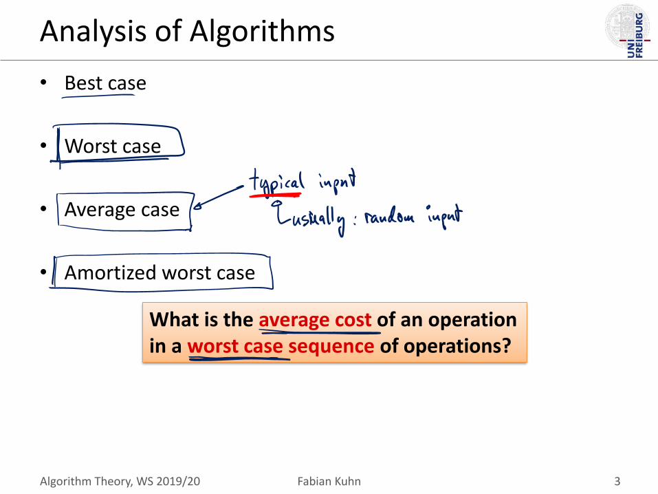
Analysis of Algorithms
• Best case
• Worst case
• Average case
• Amortized worst case
What is the average cost of an operationin a worst case sequence of operations?
Algorithm Theory, WS 2019/20 Fabian Kuhn 4
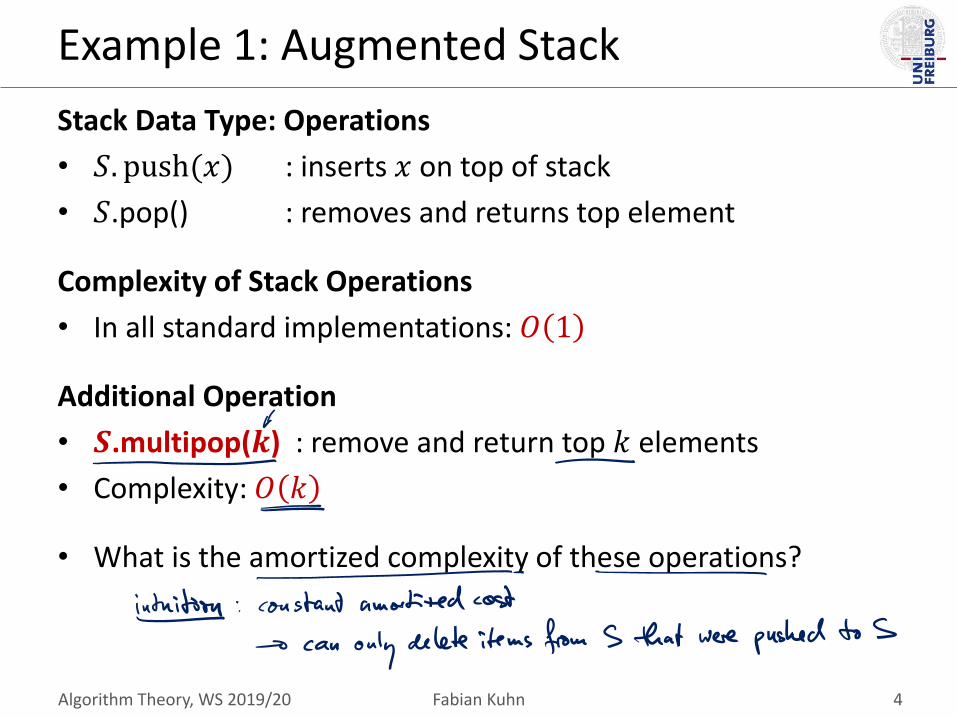
Example 1: Augmented Stack
Stack Data Type: Operations
• 𝑆. push(𝑥) : inserts 𝑥 on top of stack
• 𝑆.pop() : removes and returns top element
Complexity of Stack Operations
• In all standard implementations: 𝑂 1
Additional Operation
• 𝑺.multipop(𝒌) : remove and return top 𝑘 elements
• Complexity: 𝑂 𝑘
• What is the amortized complexity of these operations?

Algorithm Theory, WS 2019/20 Fabian Kuhn 5
Augmented Stack: Amortized Cost
Amortized Cost
• Sequence of operations 𝑖 = 1, 2, 3,… , 𝑛
• Actual cost of op. 𝑖: 𝒕𝒊• Amortized cost of op. 𝑖 is 𝒂𝒊 if for every possible seq. of op.,
𝑇 =
𝑖=1
𝑛
𝑡𝑖 ≤
𝑖=1
𝑛
𝑎𝑖
Actual Cost of Augmented Stack Operations
• 𝑆. push 𝑥 , 𝑆. pop(): actual cost 𝑡𝑖 = 𝑂(1)
• 𝑆.multipop 𝑘 : actual cost 𝑡𝑖 = 𝑂 𝑘
• Amortized cost of all three operations is constant– The total number of “popped” elements cannot be more than the total
number of “pushed” elements: cost for pop/multipop ≤ cost for push

Algorithm Theory, WS 2019/20 Fabian Kuhn 6
Augmented Stack: Amortized Cost
Amortized Cost
𝑇 =
𝑖
𝑡𝑖 ≤
𝑖
𝑎𝑖
Actual Cost of Augmented Stack Operations
• 𝑆. push 𝑥 , 𝑆. pop(): actual cost 𝑡𝑖 ≤ 𝑐
• 𝑆.multipop 𝑘 : actual cost 𝑡𝑖 ≤ 𝑐 ⋅ 𝑘

Algorithm Theory, WS 2019/20 Fabian Kuhn 7
Example 2: Binary Counter
Incrementing a binary counter: determine the bit flip cost:Operation Counter Value Cost
00000
1 00001 1
2 00010 2
3 00011 1
4 00100 3
5 00101 1
6 00110 2
7 00111 1
8 01000 4
9 01001 1
10 01010 2
11 01011 1
12 01100 3
13 01101 1

Algorithm Theory, WS 2019/20 Fabian Kuhn 8
Accounting Method
Observation:
• Each increment flips exactly one 0 into a 1
00100𝟎1111 ⟹ 00100𝟏0000
Idea:
• Have a bank account (with initial amount 0)
• Paying 𝑥 to the bank account costs 𝑥
• Take “money” from account to pay for expensive operations
Applied to binary counter:
• Flip from 0 to 1: pay 1 to bank account (cost: 2)
• Flip from 1 to 0: take 1 from bank account (cost: 0)
• Amount on bank account = number of ones We always have enough “money” to pay!
Algorithm Theory, WS 2019/20 Fabian Kuhn 9
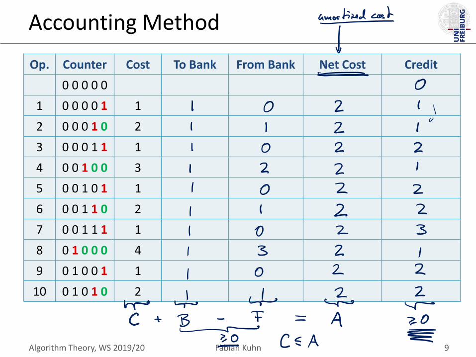
Accounting Method
Op. Counter Cost To Bank From Bank Net Cost Credit
0 0 0 0 0
1 0 0 0 0 1 1
2 0 0 0 1 0 2
3 0 0 0 1 1 1
4 0 0 1 0 0 3
5 0 0 1 0 1 1
6 0 0 1 1 0 2
7 0 0 1 1 1 1
8 0 1 0 0 0 4
9 0 1 0 0 1 1
10 0 1 0 1 0 2

Algorithm Theory, WS 2019/20 Fabian Kuhn 10
Potential Function Method
• Most generic and elegant way to do amortized analysis!– But, also more abstract than the others…
• State of data structure / system: 𝑆 ∈ 𝒮 (state space)
Potential function 𝚽:𝓢 → ℝ≥𝟎
• Operation 𝒊:– 𝒕𝒊: actual cost of operation 𝑖
– 𝑺𝒊: state after execution of operation 𝑖 (𝑆0: initial state)
– 𝚽𝒊 ≔ Φ(𝑆𝑖): potential after exec. of operation 𝑖
– 𝒂𝒊: amortized cost of operation 𝑖:
𝒂𝒊 ≔ 𝒕𝒊 +𝚽𝒊 −𝚽𝒊−𝟏

Algorithm Theory, WS 2019/20 Fabian Kuhn 11
Potential Function Method
Operation 𝒊:
actual cost: 𝑡𝑖 amortized cost: 𝑎𝑖 = 𝑡𝑖 +Φ𝑖 −Φ𝑖−1
Overall cost:
𝑇 ≔
𝑖=1
𝑛
𝑡𝑖 =
𝑖
𝑛
𝑎𝑖 +Φ0 −Φ𝑛

Algorithm Theory, WS 2019/20 Fabian Kuhn 12
Binary Counter: Potential Method
• Potential function:𝚽:𝐧𝐮𝐦𝐛𝐞𝐫 𝐨𝐟 𝐨𝐧𝐞𝐬 𝐢𝐧 𝐜𝐮𝐫𝐫𝐞𝐧𝐭 𝐜𝐨𝐮𝐧𝐭𝐞𝐫
• Clearly, Φ0 = 0 and Φ𝑖 ≥ 0 for all 𝑖 ≥ 0
• Actual cost 𝑡𝑖: 1 flip from 0 to 1
𝑡𝑖 − 1 flips from 1 to 0
• Potential difference: Φ𝑖 −Φ𝑖−1 = 1 − 𝑡𝑖 − 1 = 2 − 𝑡𝑖
• Amortized cost: 𝑎𝑖 = 𝑡𝑖 +Φ𝑖 −Φ𝑖−1 = 2