Chapter 35: Sediment Transport in Open Channels - Freefreeit.free.fr/The Civil Engineering...

35Sediment Transport

in Open Channels

35.1 Introduction 35.2 The Characteristics of Sediment

Density, Size, and Shape • Size Distribution • Fall (or Settling) Velocity • Angle of Repose

35.3 Flow Characteristics and Dimensionless Parameters; Notation

35.4 Initiation of MotionThe Shields Curve and the Critical Shear Stress • The Effect of Slope • Summary

35.5 Flow Resistance and Stage-Discharge PredictorsForm and Grain Resistance Approach • Overall Resistance Approach • Critical Velocity • Summary

35.6 Sediment TransportSuspended Load Models • Bed-Load Models and Formulae • Total Load Models • Measurement of Sediment Transport • Expected Accuracy of Transport Formulae

35.7 Special Topics Local Scour • Unsteady Aspects • Effects of a Nonuniform Size Distribution • Gravel-Bed Streams

35.1 Introduction

The erosion, deposition, and transport of sediment by water arise in a variety of situations with engi-neering implications. Erosion must be considered in the design of stable channels or the design for localscour around bridge piers. Resuspension of possibly contaminated bottom sediments have consequencesfor water quality. Deposition is often undesirable since it may hinder the operation, or shorten theworking life, of hydraulic structures or navigational channels. Sediment traps are specifically designedto promote the deposition of suspended material to minimize their downstream impact, e.g., on coolingwater inlet works, or in water treatment plants. A large literature exists on approaches to problemsinvolving sediment transport; the following can only introduce the basic concepts in summary fashion.It is oriented primarily to applications in steady uniform flows in a sand-bed channel; problems involvingflow nonuniformity, unsteadiness, and gravel-beds, are only briefly mentioned and coastal processes aretreated in the section on coastal engineering. Cohesive sediments, for which physico-chemical attractiveforces may lead to the aggregation of particles, are not considered at all. The finer fractions (clays andsilts, see Section 35.2) that are susceptible to aggregation are found more in estuarial and coastal shelfregions rather than in streams. A recent review of problems in dealing with cohesive sediments is givenby Mehta et al. (1989 a, b).

D. A. LynPurdue University

© 2003 by CRC Press LLC

35

-2

The Civil Engineering Handbook, Second Edition

35.2 The Characteristics of Sediment

Density, Size, and Shape

The density of sediment depends on its composition. Typical sediments in alluvial water bodies consistmainly of quartz, the specific gravity of which can be taken as s = 2.65. The specific weight is thereforegs = 165.4 lb/ft,3 or 26.0 kN/m.3 In many formulae, the effective specific weight, which includes the effectof buoyancy, is used, i.e., (s-1)g, where g is the specific weight of water.

The exact shape of a sediment particle is not spherical, and so a compact specification of its geometryor size is not feasible. Two practical measures of grain size are: (i) the sedimentation or aerodynamicdiameter — the diameter of the sphere of the same material with the same fall velocity, ws, (see belowfor definition) under the same conditions, and (ii) the sieve diameter — the length of a side of the squaresieve opening through which the particle will just pass. Because size determination is most often per-formed with sieves, the available data for sediment size usually refer to the sieve diameter, which is takento be the geometric mean of the adjacent sieve meshes, i.e., the mesh size through which the particle haspassed, and the mesh size at which the particle is retained. The sedimentation diameter is relatedempirically to the sieve diameter by means of a shape factor, S.F., which increases from 0 to 1 as theparticle becomes more spherical (for a well-worn sand, S.F. ª 0.7).

Size Distribution

Naturally occurring sediment samples exhibit a range of grain diameters. A characteristic diameter, da,may be defined in terms of the percent, a, by weight of the sample that is smaller than da. Thus, for asample with d84 = 0.35 mm, 84% by weight of the sample is less than 0.35 mm in diameter. The mediansize is denoted as d50. Frequently, the grain size distribution is assumed to be lognormally distributed,and a geometric mean diameter and standard deviation are defined as dg = , and sg = .For a lognormal distribution, d50 = dg, and the arithmetic mean diameter, dm = dge0.5ln(2sg). Similarly, da

can be determined from dg and sg from the relation, da = dg sgZa , where Za is the standard normal variate

corresponding to the value of a. For example, if a = 65%, dg = 0.35 mm, and sg = 1.7, then Za = 0.39,and so d65 = (0.35 mm)(1.7)0.39 = 0.43 mm. In natural sand-bed streams, sg typically ranges between1.4 and 2, but in gravel-bed streams, it may attain values greater than 4. Qualitative discussions ofsediment size may be based on a standard sediment grade scale terminology established by the AmericanGeophysical Union. A simplified grade scale divides the size range into cobbles and boulders (d > 64 mm),gravels (2 mm < d < 64 mm), sands (0.06 mm < d < 2 mm), silts (0.004 mm < d < 0.06 mm), and clays(d < 0.004 mm).

Fall (or Settling) Velocity

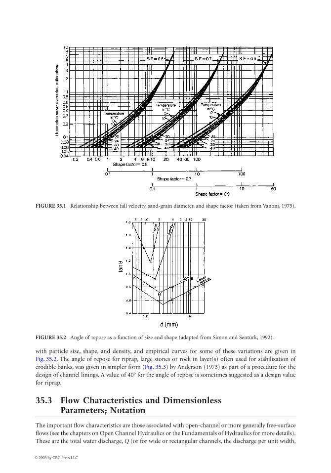
The terminal velocity of a particle falling alone through a stagnant fluid of infinite extent is called its fallor settling velocity, ws. The standard drag curve for a spherical particle provides a relationship betweend and ws (see chapter on Fundamentals of Hydraulics). For non-spherical sand particles in water, the fallvelocity at various temperatures can be determined from Fig. 35.1 if the sieve diameter and S.F. are knownor can be assumed (note the different fall velocity scales). As an example, for a geometric sieve diameterof 0.3 mm and a shape factor, S.F. = 0.7, the fall velocity in water at 10∞C is determined as ª 3.6 cm/s.In a horizontally flowing turbulent suspension, the actual mean fall velocity of a given particle may beinfluenced by neighboring particles (hindered settling) and by turbulent fluctuations.

Angle of Repose

The angle of repose of a sediment particle is important in describing the initiation of its motion andhence sediment erosion of an inclined surface, such as a stream bank. It is defined as the angle, q, atwhich the particle is just in equilibrium with respect to sliding due to gravitational forces. It will vary

d16d84 d84 d16§


Sediment Transport in Open Channels

35

-3

with particle size, shape, and density, and empirical curves for some of these variations are given inFig. 35.2. The angle of repose for riprap, large stones or rock in layer(s) often used for stabilization oferodible banks, was given in simpler form (Fig. 35.3) by Anderson (1973) as part of a procedure for thedesign of channel linings. A value of 40° for the angle of repose is sometimes suggested as a design valuefor riprap.

35.3 Flow Characteristics and Dimensionless Parameters; Notation

The important flow characteristics are those associated with open-channel or more generally free-surfaceflows (see the chapters on Open Channel Hydraulics or the Fundamentals of Hydraulics for more details).These are the total water discharge, Q (or for wide or rectangular channels, the discharge per unit width,

FIGURE 35.1 Relationship between fall velocity, sand-grain diameter, and shape factor (taken from Vanoni, 1975).

FIGURE 35.2 Angle of repose as a function of size and shape (adapted from Simon and Sentürk, 1992).


35

-4

The Civil Engineering Handbook, Second Edition

q = Q/B, where B is the width of the channel), the mean velocity, V = Q/A, where A is the channel cross-sectional area, the hydraulic radius, Rh, (or for a very wide channel the flow depth, Rh ª H), and theenergy or friction slope, Sf . The total bed shear stress, tb, and the related quantities, the shear velocity,u* = = , where g is the gravitational acceleration, and friction factor, f = 8(u*/V)2, are alsoimportant.

Much of sediment transport engineering remains highly empirical, and so the organization of infor-mation in terms of dimensionless parameters becomes important (see the discussion of dimensionalanalysis in the chapter on Fundamentals of Hydraulics). Sediment and flow quantities may be combinedin several dimensionless parameters that arise repeatedly in sediment transport. A dimensionless bedshear stress, also termed the Shields parameter (see Section 35.4), can be defined as

(35.1)

Two grain Reynolds numbers based on the grain diameter can be usefully defined as

(35.2)

where n is the fluid kinematic viscosity. Since Re2g µ d 3, a definition of a dimensionless diameter may be

motivated as d* = Reg2/3.

A grain ‘Froude’ number also based on grain diameter can be defined as

(35.3)

A dimensionless sediment discharge per unit width, F, may be defined as:

(35.4)

where gs = gqC—

is the weight flux of sediment per unit width and—

C is the flux-weighted mass or weightconcentration of sediment (see Section 35.6 for more details).

In the above definitions, various characteristic grain diameters and shear velocities may be usedaccording to the context.

FIGURE 35.3 Angle of repose for riprap (from Anderson, 1973).

tb r§ gRhSf

Q ∫-( ) =

-( ) =-( )

tg

b h f

s d

u

g s d

R S

s d1 1 1

2*

Re Re**

g

g s d u d∫-( )

∫1 3

n n and

FrV

g s d

V

u fg ∫ -( )=

ÊËÁ

ˆ¯̃

=1

8

*

Q Q

F ∫-( )

g

g s d

s sg

1 3


Sediment Transport in Open Channels 35-5

35.4 Initiation of Motion

The Shields Curve and the Critical Shear Stress

A knowledge of the hydraulic conditions under which the transport of sediment in an alluvial channelbegins or is initiated is important in numerous applications, such as the design of stable channels, i.e.,channels that will not suffer from erosion, or bank stabilization, or remedial measures for scour. Acriterion for the initiation of general sediment transport in a turbulent channel flow may be given interms of a critical bed shear stress, (tb)c = r(u*)2

c , above which general motion of bed sediment of meandiameter, d, is observed. The Shields curve (Fig. 35.4) correlates a critical dimensionless bed shear stress,Qc, to a critical grain Reynolds number, (Re*)c, where (u*)c is used in defining both Qc and (Re*)c. TheShields curve is an implicit relation, and so a solution for (u*)c must be obtained iteratively. For large(Re*)c (i.e., for coarse sediment), Qc Æ ª0.06, which provides a convenient initial guess for iteration. Alsodrawn on Fig. 35.4 are straight oblique lines along which an auxiliary parameter, (d/n) =

is constant. This parameter does not involve (u*)c, and so, provided d and n are known, (u*)c

can be directly determined by the intersection of these lines with the Shields curve. Various formulae orcurve-fits have been proposed for describing the Shields curve; one example is due to Brownlie (1981)and involves the auxiliary parameter, Y ∫ Reg

–0.6,

(35.5)

Example 35.1

Given a sand (s = 2.65) grain with d = 0.4 mm in water with n = 0.01 cm2/s, what is the critical shear stress?The iterative procedure based on the graphical Shields curve starts with an initial guess, Qc = 0.06, implying(u*

2)c = 2.0 cm2/s2 and (Re*)c = 7.9. This is inconsistent with the Shields curve, which indicates Qc = 0.032for (Re*)c = 7.9. The procedure is iterated by making another guess, Qc = 0.032, which yields (tb)c = 0.21kPa corresponding to (Re*)c = 5.8. This result is sufficiently consistent with the Shield curve, and so the

FIGURE 35.4 The Shields diagram relating critical shear stress to hydraulic and particle characteristics (adaptedfrom ASCE Sedimentation Engineering, 1975).

0.1g s 1–( )d0.1Reg

QcYY= + ¥ -0 22 0 06 10 7 7. . .


35-6 The Civil Engineering Handbook, Second Edition

iteration can be stopped. More directly, the auxiliary parameter, (d/n) = 10, can be computed,and the line corresponding to this value intersects the Shields curve at Qc = 0.034. The use of the Brownlieempirical formula (Eq. [35.5]) gives, with Reg = 32.2 and Y = 0.125, more directly Qc = 0.034.

Instead of using (tb)c, traditional procedures for the design of stable channels have often been formu-lated in terms of a critical average velocity, Vc, or critical unit-width discharge, qc, above which sedimenttransport begins, because these quantities are more easily available than the bed shear stress. If a rela-tionship between V and tb, namely a friction or flow resistance law, then Vc can be derived from (tb)c,and this is discussed in Section 35.5.

The Effect of Slope

The above criterion is applicable to grains on a surface with negligible slope, as is usually the case forgrains on the channel bed. Where the slope of the surface on which grains are located is appreciable,e.g., on a river bank, its effect cannot be neglected. With the inclusion of the additional gravitationalforces, a force balance reveals that (tb)c is reduced by a fraction involving the angle of repose of the grain,and the ratio of the value of (tb)c including slope effects to its value for a horizontal surface is given by:

(35.6)

where f = the angle of the sloping surfaceq = the angle of repose of the grain.

On a horizontal surface, f = 0, and the ratio is unity, whereas if f = q, then no shear is required toinitiate sediment motion (consistent with the definition of the angle of repose).

Summary

Although the Shields curve is widely accepted as a reference, controversy remains concerning its detailsand interpretation, e.g., its behavior for small (Re*)c (Raudkivi, 1990) and the effect of fluid temperature(Taylor and Vanoni, 1972). The random nature of turbulent flow and random magnitudes of the instan-taneous bed shear stresses motivate a probabilistic approach to the initiation of sediment motion. Thecritical shear stress given by the Shields curve can be accordingly interpreted as being associated with aprobability that sediment particle of given size will begin to move. It should not be interpreted as acriterion for zero sediment transport, and design relations for zero transport, if based on the Shieldscurve, should include a significant factor of safety (Vanoni, 1975).

35.5 Flow Resistance and Stage-Discharge Predictors

The stage-discharge relationship or rating curve for a channel relating the uniform-flow water level (stage)or hydraulic radius, Rh, to the discharge, Q, is determined by channel flow resistance. For flow conditionsabove the threshold of motion, the erodible sand bed is continually subject to scour and deposition, sothat the bed acts as a deformable or ‘movable’ free surface. The plane bed, i.e., one in which large-scalefeatures are absent, is often unstable, and bedforms (Fig. 35.5) such as dunes, ripples, and antidunes,develop. Dunes, which exhibit a mild upstream slope and a sharper downstream slope, are the mostcommonly occurring of bedforms in sand-bed channels. Ripples share the same shape as dunes, but aresmaller in dimensions. They may be found in combination with dunes, but are generally thought to beunimportant except in streams at small depths and low velocities. Antidunes assume a smoother moresymmetric sinusoidal shape, which results in less flow resistance, and are associated with steeper streams.Antidunes differ from dunes in moving upstream rather than downstream, and in being associated withwater surface variations that are in phase rather than out of phase with bed surface variations.

0.1g s 1–( )d

Kslope

b c slope

b c zero slope

=( )[ ]

( )[ ] = -ÊËÁ

ˆ¯̃

t

tfq

12

2

1 2sin

sin

/



In fixed-bed open-channel flows, resistanceis characterized by a Darcy-Weisbach frictionfactor, f (see chapter on Fundamentals ofHydraulics) or a Manning’s n (see chapter onOpen Channel Hydraulics), which is assumedto vary only slowly or not at all with discharge.For movable or erodible beds, substantialchanges in flow resistance may occur as thebedforms develop or are washed out. Veryloosely, as transport intensity (as measured,e.g., by the Shields parameter, Q) increases, rip-ples evolve into dunes, which in turn becomeplane or transition beds, to be followed by anti-dunes. Multiple depths may be consistent withthe same discharge or velocity (Fig. 35.6), andthe rating curve (the relationship between stageor depth and discharge or velocity) may exhibitdiscontinuities. These discontinuities areattributed to a short-term transition from low-velocity high-resistance flow over ripples anddunes, termed lower-regime flow, to high-velocity low-resistance flow over plane, transition or antidunebed, termed upper-regime flow or vice-versa. Because of these two possible regimes, movable-bed frictionformulae (unlike fixed-bed friction formulae) must include a method to determine the flow regime.

Form and Grain Resistance Approach

In flows over dunes and ripples, form resistance due to flow separation from dune tops provides thedominant contribution to overall resistance. Yet the processes involved in determining bedform charac-teristics are more directly related to the actual bed shear stress (as in the problem of initiation of motion).Much of sediment transport modeling has distinguished between form and grain (skin) resistance (seethe section on hydrodynamic forces in the chapter on Fundamentals of Hydraulics for the distinctionbetween the two types of flow resistance). An overall bed shear stress, (tb)overall ∫ g Rj Sf , is taken as thesum of a contribution due to grain resistance, t¢, and a contribution due to form resistance, t≤. Since(tb)overall is usually correlated empirically with t¢, it remains only to determine t¢ from given hydraulicparameters. The traditional approach estimates t¢ from fixed-bed friction formulae for plane beds. Asimple effective example of this approach to stage-discharge prediction is due to Engelund and Hansen(1967) (with extension by Brownlie (1983)) and correlates a total overall dimensionless shear stress, Q,with a dimensionless grain shear stress, Q¢:

FIGURE 35.5 Various bedforms.

FIGURE 35.6 Stage-discharge data reported by Dawdy(1961) for the Rio Grande River near Bernalillo, New Mexico.(Adapted from Brownlie, 1981.)



Engelund-Hansen formula

(35.7a)

(35.7b)

(35.7c)

where Q¢(∫ Rh¢Sf /(s-1) d50) is related to V by a friction formula for a plane fixed bed:

(35.8)

The lower regime corresponds to flows over dune-covered beds with dominant contribution due toform resistance, such that Q > Q¢ for values of Q¢ not too close to 0.06, whereas in the transition orupper regime, corresponding to plane beds or beds with antidunes, Q = Q¢, because flow resistance isexpected to be due primarily to grain resistance, comparable in this respect to plane beds. The Engelund-Hansen formula was originally developed based on large-flume laboratory data with d50 in the range 0.19mm to 0.93 mm, and sg of 1.3 for the finest sediment and 1.6 for the others.

Overall Resistance Approach

The distinction between grain (skin) and form resistance is physically sound, but the use of a plane fixed-bed friction formula such as Eq. (35.8) cannot be justified rigorously for beds with dunes and ripples, andthe need for a further correlation between Q and Q¢ is inconvenient. A simpler more direct approach relatingQ (or Rh) directly to Q or other dimensionless parameters may therefore be more attractive from an engi-neering point of view. Guided by dimensional analysis, Brownlie (1983) performed regression analyses on alarge data set of laboratory and field measurements, and proposed the following stage-discharge formulae:

Brownlie formulae

(35.9a)

(35.9b)

where sg = the geometric standard deviationFrg = the grain Froude number (Eq. [35.3])

To determine whether the flow is in lower or upper regime, the following criteria are applied:

• for Sf > 0.006, only upper regime flow is observed,

• for Sf < 0.006, additional criteria are formulated in terms of a modified grain Froude number,Fr*

g ∫ Frg /[1.74Sf–1/3], and a modified grain Reynolds number, D ∫ u¢*d50 /(11.6n), where u¢* is the

shear velocity corresponding to the upper regime flow, i.e., due primarily to grain resistance.

• the lower limit of the upper regime is given as

(35.10a)

(35.10b)

Q Q Q= ¢ - £ ¢ £ ( )1 58 0 06 0 06 0 55. . , . . , lower regime

, . , = ¢ £ ¢ £ ( )Q Q0 55 1 upper regime

. . . .

= ¢( ) -[ ] £ ¢ ( )-1 425 0 425 1

1 8 1 8

Q Q upper regime

V

gR S

R

dh f

h

¢= ¢

5 765 51

1065

. log.

R

ds Fr Sh

g f g50

0 95 1 89 0 74 0 30 0576 1= -( ) -. ,. . . .s lower regime,

. ,. . . .= -( ) -0 0348 1

0 83 1 67 0 77 0 21s Fr Sg f gs upper regime,

log . . log . log , *10 10 10

20 0247 0 152 0 838 2Frg up

( ) = - + + ( ) <D D D

= ≥log . , 101 25 2D



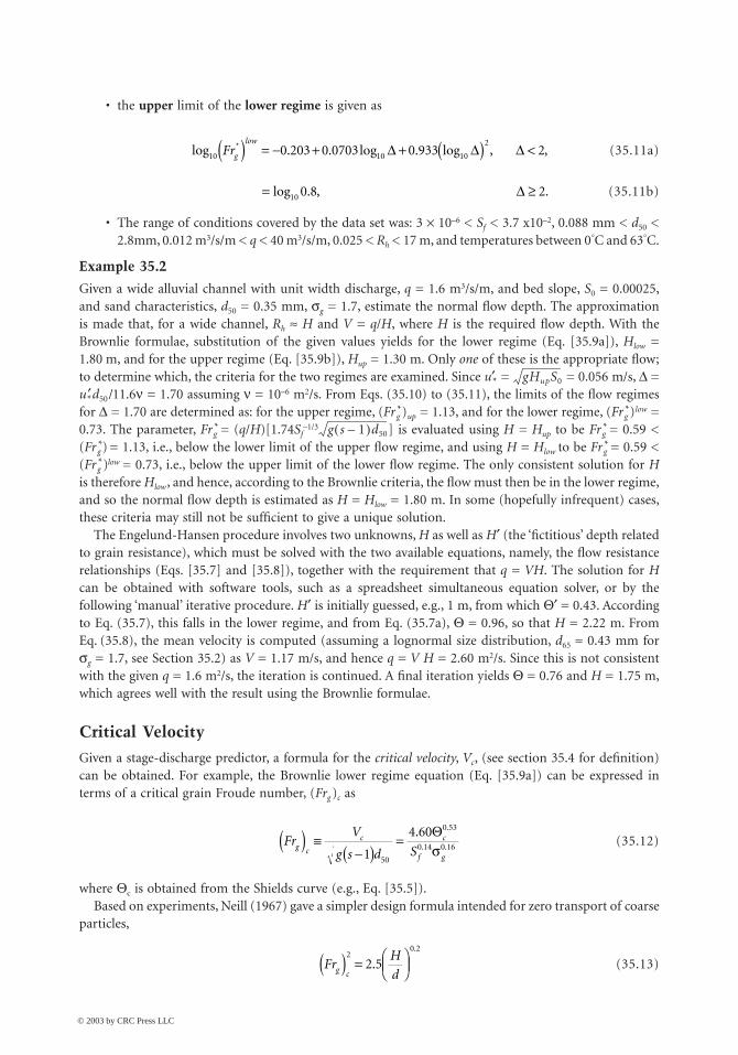
• the upper limit of the lower regime is given as

(35.11a)

(35.11b)

• The range of conditions covered by the data set was: 3 ¥ 10–6 < Sf < 3.7 x10–2, 0.088 mm < d50 <2.8mm, 0.012 m3/s/m < q < 40 m3/s/m, 0.025 < Rh < 17 m, and temperatures between 0∞C and 63∞C.

Example 35.2

Given a wide alluvial channel with unit width discharge, q = 1.6 m3/s/m, and bed slope, S0 = 0.00025,and sand characteristics, d50 = 0.35 mm, sg = 1.7, estimate the normal flow depth. The approximationis made that, for a wide channel, Rh ª H and V = q/H, where H is the required flow depth. With theBrownlie formulae, substitution of the given values yields for the lower regime (Eq. [35.9a]), Hlow =1.80 m, and for the upper regime (Eq. [35.9b]), Hup = 1.30 m. Only one of these is the appropriate flow;to determine which, the criteria for the two regimes are examined. Since u¢* = = 0.056 m/s, D =u ¢*d50/11.6n = 1.70 assuming n = 10–6 m2/s. From Eqs. (35.10) to (35.11), the limits of the flow regimesfor D = 1.70 are determined as: for the upper regime, (Fr*

g )up = 1.13, and for the lower regime, (Fr*g )low =

0.73. The parameter, Fr*g = (q/H)[1.74Sf

–1/3 ] is evaluated using H = Hup to be Fr*g = 0.59 <

(Fr*g ) = 1.13, i.e., below the lower limit of the upper flow regime, and using H = Hlow to be Fr*

g = 0.59 <(Fr*

g )low = 0.73, i.e., below the upper limit of the lower flow regime. The only consistent solution for His therefore Hlow, and hence, according to the Brownlie criteria, the flow must then be in the lower regime,and so the normal flow depth is estimated as H = Hlow = 1.80 m. In some (hopefully infrequent) cases,these criteria may still not be sufficient to give a unique solution.

The Engelund-Hansen procedure involves two unknowns, H as well as H¢ (the ‘fictitious’ depth relatedto grain resistance), which must be solved with the two available equations, namely, the flow resistancerelationships (Eqs. [35.7] and [35.8]), together with the requirement that q = VH. The solution for Hcan be obtained with software tools, such as a spreadsheet simultaneous equation solver, or by thefollowing ‘manual’ iterative procedure. H¢ is initially guessed, e.g., 1 m, from which Q¢ = 0.43. Accordingto Eq. (35.7), this falls in the lower regime, and from Eq. (35.7a), Q = 0.96, so that H = 2.22 m. FromEq. (35.8), the mean velocity is computed (assuming a lognormal size distribution, d65 ª 0.43 mm forsg = 1.7, see Section 35.2) as V = 1.17 m/s, and hence q = V H = 2.60 m2/s. Since this is not consistentwith the given q = 1.6 m2/s, the iteration is continued. A final iteration yields Q = 0.76 and H = 1.75 m,which agrees well with the result using the Brownlie formulae.

Critical Velocity

Given a stage-discharge predictor, a formula for the critical velocity, Vc, (see section 35.4 for definition)can be obtained. For example, the Brownlie lower regime equation (Eq. [35.9a]) can be expressed interms of a critical grain Froude number, (Frg )c as

(35.12)

where Qc is obtained from the Shields curve (e.g., Eq. [35.5]). Based on experiments, Neill (1967) gave a simpler design formula intended for zero transport of coarse

particles,

(35.13)

log . . log . log , ,*10 10 10

20 203 0 0703 0 933 2Frg

low( ) = - + + ( ) <D D D

= ≥log . , .10 0 8 2D

gHupS0

g s 1–( )d50

FrV

g s d Sg c

c c

f g

( ) ∫-( )

=1

4 60

50

0 53

0 14 0 16

. .

. .

Qs

FrH

dg c( ) = Ê

ËÁˆ¯̃

20 2

2 5..



This gives a more conservative result than the Eq. (35.12). A design equation for sizing riprap, verysimilar to Eq. (35.13), and recommended by the U. S. Army Corps of Engineers (1995) is

(35.14a)

where KR is an empirical coefficient correcting for various effects such as the vertical velocity distributionand the thickness of the riprap layer, as well as including a safety factor. Although Eq. (35.6) (with q =40°) may be used for evaluating Kslope, this is found to be rather conservative, and an empirical curve forthis factor has been developed.

Example 35.3

A channel is to be designed to carry a discharge of 5 m3/s on a slope of 0.001. The bed material has amedian diameter, d50 = 8 mm, and a geometric standard deviation, sg = 3. Determine the width anddepth at which the channel will not erode. Assume for simplicity a rectangular channel cross-section andrigid banks. For d50 = 8 mm, it is found from Eq. (35.5) that Qc = 0.054, so from Eq. (35.12), (Frg)c =2.18 and Vc = 0.78 m/s. This is substituted into the lower regime friction equation, Eq. (35.9a), to giveRh = BH/(B+2H) = 0.72 m. Since Q = Vc BH = 5 m3/s, H is determined as 0.9 m, and so B = 7.1 m. IfEq. (35.13) is used with a Manning-Strickler friction law, then H is found to be 0.46 m, and B to be12.4 m, with Vc = 0.86 m/s. Eq. (35.12), being based on Shields curve, is not intended to be used fordesign for zero transport (see previous remarks in section 35.4), while Eq. (35.13) was intended as adesign equation for zero transport and so gives a more conservative value (smaller H and hence smallerbed shear stress for given bed slope).

Summary

The prediction of flow depth in alluvial channels remains an uncertain art with much room for judgement.Estimates using various predictors should be considered and the use of field data specific to the problemshould be exploited where feasible to arrive at a range of predictions. If the regime is correctly predicted,the better stage-discharge relations are generally reliable to within 10 to 15% in predicting depth.

35.6 Sediment Transport

Three modes of sediment transport are distinguished: wash load, suspended load, and bed load. Washload refers to very fine suspended material, e.g., silt, that because of their very small fall velocities, interactslittle with the bed. It will not be further considered since it is determined by upstream supply conditionsrather than by local hydraulic parameters. Suspended load refers to material that is transported down-stream primarily in suspension far from the bed, but which because of sedimentation and turbulentmixing still interacts significantly with the bed. Finally, bed load refers to material that remains generallyclose to the bed in the bedload region, being transported mainly through rolling or in short hops (termedsaltation). The relative importance of the two modes of sediment transport may be roughly inferred fromthe ratio of settling velocity to shear velocity, ws/u*. For ws/u* < 0.5, suspended load transport is likelydominant, while for ws/u* > 1.5, bedload transport is likely dominant. The sum of suspended and bedloads is termed bed-material load as distinct from the wash load, which may only be very weakly, if atall, related to material found in bed samples.

The total sediment load or discharge, GT, is considered here as the sum of only the suspended-loaddischarge, GS, and the bedload discharge, GB, and is defined as the mass or more usually the weight fluxof sediment material passing a given cross-section (SI units of kg/s or N/s, English units slugs/s or lb/s).A total sediment discharge (by weight) per unit width, based on the flux over the entire depth. is often used:

d

HK

V

K s HR

slope

30

2 5

1=

-( )Ê

ËÁÁ

ˆ

¯˜˜

.



(35.14b)

where u and c = the mean velocity and mass (or weight) concentration at a point in the water column—

C = a mean flux-weighted mass (or weight) concentration defined by Eq. (35.14a).

Because of a nonuniform velocity profile,—

C is not equal to the depth-averaged concentration, ·CÒ ∫ (1/H)Ú0

H c dy.

Suspended Load Models

The prediction of gT given appropriate sediment characteristics and hydraulic parameters has beenattempted by treating bed load and suspended load separately, but such an approach is fraught withdifficulties. The traditional approach derives a differential equation for conservation of sediment assum-ing uniform conditions in the streamwise direction:

(35.15)

where es is a turbulent diffusion or mixing coefficient for sediment. The first term represents a net upward sediment flux due to turbulent mixing, while the second term

is interpreted as the net downward flux due to settling. A solution for the vertical distribution of sedimentconcentration, c(y), depends on a model for es, and a boundary condition at or near the bed. The well-known Rouse concentration profile,

(35.16)

with the Rouse exponent, ZR ∫ ws/bku*, assumes an eddy viscosity mixing model with es = bu* y(1 – y/H),where b is a coefficient relating momentum to sediment diffusion, and the von Kármán constant, k,stems from the assumption of a log-law velocity profile. It avoids a precise specification of the bottomboundary condition by introducing a reference concentration, cref , at a reference level y = yref , taken closeto the bed. Here u* = refers to the overall shear velocity (i.e., not only the shear velocity associatedwith grain resistance).

Although Eq. (35.16) can usually be made to fit measured concentration profiles approximately withan appropriate choice of ZR, its predictive use is limited by the lack of information concerning b, k, andparticularly cref , which may vary with hydraulic and sediment characteristics. In the simplest models, b = 1and k = 0.4, which assume that sediment diffusion is identical to momentum diffusion and the velocityprofile follows the log-law (see section on turbulent flows in the chapter on fundamentals of hydraulics)profile exactly as in plane fixed-bed flows without sediment. More complicated models (e.g., van Rijn,1984a) have been proposed in which b is correlated with ws/u* and k varies with suspended sedimentconcentration. The suspended load discharge per unit width may be computed using Eq. (35.16) as

(35.17)

with u typically assumed to be described by a log-law profile. To determine the total load (per unit width),gT, a formula for predicting gB, the transport per unit width in the bed-load region, 0 < y < yref , mustbe coupled with Eq. (35.17), and the reference level, yref , must be chosen at the limit of the bed loadregion. In flows with bed forms, neither Eq. (35.15) nor Eq. (35.16) can be rigorously justified, since bed

g qC u c dyT

H

= = Úg g 0

es s

dc

dyw c+ = 0

c y

c

H y

y

y

H yref

ref

ref

ZR( ) = --

Ê

ËÁ

ˆ

¯˜

gRhSf

g u c dysy

H

ref

= Úg



conditions are not uniform in the streamwise direction and the log-law velocity profile is inadequate todescribe velocity and stress profiles near the bed (Lyn, 1993).

Bed-Load Models and Formulae

Bed-load models are used either in cases where bed load transport is dominant, or to complementsuspended-load models in total-load computations. Most available formulae can be written in terms ofthe dimensionless bed-load transport, Fb, and a dimensionless grain shear stress, Q¢ (see Section 35.2for definitions). Only two such models, one traditional and one more recent, are described. The Meyer-Peter-Muller bed-load formula was based on laboratory experiments with coarse sediments (meandiameter range: 0.4 to 30 mm) with very little suspended load.

Meyer-Peter-Muller bed-load formula

(35.18)

where the dimensionless critical shear stress, Qc = 0.047 (note the difference from the generally acceptedShields’ curve value of 0.06 for coarse material) and Q¢ is the fraction of the dimensionless total shearstress, Q¢ = (k/k¢)3/2Q, that is attributed to grain resistance. Based on a plane fully rough fixed-bed frictionlaw of Strickler type, the fraction, k/k¢, is computed from

(35.19)

In the Meyer-Peter-Muller formula, the characteristic grain size used in defining Fb and Q¢ is the meandiameter, dm (which can be related to dg if necessary, see Section 35.2).

A more recent bed-load model due to van Rijn (1984), intended both for predicting bed-load domi-nated transport as well as for complementing a suspended-load model, is similar in form:

van Rijn bed-load formula

(35.20)

Qc is determined from a Shields curve relation, and Q¢ is computed from a fully rough plane-bed frictionformula of log-law form (cf. Eq. [35.8]),

(35.21)

where the equivalent roughness height, ks = 3 d90. The median grain diameter, d50, is used in definingFb, Q¢, and Reg. In tests with laboratory and field data, Eq. 35.20 performed on average as well as otherwell-known bed-models including the Meyer-Peter-Muller formula. Equating qB to a sediment flux basedon a reference mass concentration, cref, at a reference level (y = yref), van Rijn (1984b) obtained an semi-empirical relation for cref to be used with a suspended-load model

(35.22)

F QQ

QQb

c c

= ¢ -ÊËÁ

ˆ¯̃

¢ ≥0 08 1 1

3 2

. , ,

/

k

k

d

R

U

gR Sh h f¢

=ÊËÁ

ˆ¯̃

0 12 90

1 6

.

/

FQ Q Q

Qb

c

g c

=¢( ) -[ ] ¢ ≥0 053

11

2 1

0 2.Re

, .

.

.

V

u

R

kh

s¢=

*

. log5 7512

10

c sd

y Rerefref

c

g c

=Ê

ËÁ

ˆ

¯˜

¢( ) -[ ] ¢ ≥0 0151

150

1 5

0 2. , ,

.

. Q Q Q

Q



where yref is chosen to be one-half of a bed form height for lower regime flows, or the roughness heightfor upper regime flows with a minimum value chosen arbitrarily to be 0.01 H.

Example 35.4

Given quartz (s = 2.65) sediment with d50 = 1.44 mm, sg = 2.2, in a uniform flow of hydraulic radius,Rh = 0.62 m, in a wide channel of slope, S = 0.00153, and average velocity, V = 0.8 m/s, what is thesediment discharge per unit width? A bed-load dominated sediment discharge is indicated by w/u* ª(16 cm/s)/(9.6 cm/s) = 1.6, based on d50, and u* = = 0.096 m/s. In the Meyer-Peter-Muller formula,k/k¢ = 0.43, where d90 = 3.9 mm and u* = 0.096 m/s. Hence, since dm = 1.96 mm, it is found that Q¢ =0.082. This gives Fb = 0.052 from which gB = gsFb = 0.47 N/s/m or

—

C = gb/gq = 97 ppm bymass. If the van Rijn formula is used, u¢* = 0.050 m/s, so that Q¢ = 0.106. From the Shields curve, Qc =0.039 for Rg = 219, so that Fb = 0.056 or gb = 0.32 N/s/m or

—

C = 66 ppm. The given parameter valuescorrespond to field measurements in the Hii River in Japan where the reported

—

C was 191 ppm (fromthe data compiled by Brownlie, 1981), which may have included some suspended load as well as wash load.

Total Load Models

The distinction between suspended load and bed load is conceptually useful, but, as has been notedpreviously in other contexts, this does not necessarily yield any predictive advantages since neithercomponent can as yet be treated satisfactorily for most practical problems. As such, simpler empiricalformulae that directly relate gT (or equivalently,

—

C ) to sediment and hydraulic parameters remain attrac-tive and have often performed as well or better than more complicated formulae in practical predictions.Only two of the many such formulae will be discussed. The formula of Engelund and Hansen (1967)was developed along with their stage-discharge formula (see Section 35.5 for the range of experimentalparameters). The total dimensionless transport per unit width, FT, is related to Frg, and Q, with char-acteristic grain size, dg, by

Engelund-Hansen total-load formula

(35.23)

The Brownlie formula was originally stated in terms of the mean sediment transport (mass or weight)concentration,

—

C, as:

Brownlie total-load formula

(35.24)

where cf = 1 for laboratory data and cf = 1.27 for field data, (Frg)c is the critical grain Froude numbercorresponding to the initiation of sediment motion given by Eq. (35.12). In term of FT and Q, Eq. (35.24)can be expressed (assuming Rh ª H) with rounding as

(35.25)

Example 35.5

The total load formulae should also be applicable to bed-load dominated transport as in Example 35.3. Inthat case, the Engelund-Hansen formula, with Frg

2 = 27.5 and Q = 0.4, predicts FT = 0.35, correspondingto gT = 2.0 N/s/m and

—

C = 411 ppm by weight. This is approximately twice the measured value. The Brownlieformula, with (Frg)c = 1.8 from Eq. 35.12 and cf = 1.27, yields FT = 0.16, corresponding to gT = 0.91 N/s/mor in terms of

—

C = 189 ppm by weight, which agrees well with the measured value of 191 ppm. This rather

gHS

g s 1–( )dm3

F QT gFr= 0 05 2 3 2. /

C c Fr Fr Sd

Rf g g c fh

= - ( )[ ] ÊËÁ

ˆ¯̃

0 007121 98

0 66 50

0 33

..

.

.

Q QTf

g g c g

c

sFr Fr Fr s=

ÊËÁ

ˆ¯̃

- ( )[ ] -( )[ ]0 00712 12 0 1 5

.. .



close agreement should be considered somewhat fortuitous, and is at least partially attributed to the factthat the observed value was included in the data set on which the Brownlie formulae were based. Theperformance of the Brownlie formulae in practice is likely to be similar to the better recent proposals.

Measurement of Sediment Transport

In addition to, and contributing to, the difficulties in describing and predicting accurately sediment trans-port, total load measurements, particularly in the field, are associated with much uncertainty. Naturalalluvial channels may exhibit a high degree of spatial and temporal nonuniformities, which are not specif-ically considered in the ‘averaged’ models discussed above. Standard methods of suspended load measure-ments in streams include the use of depth-integrating samplers that collect a continuous sample as theyare lowered at a constant rate (depending on stream velocity) into the stream, and the use of point-integrating samplers that incorporate a valve mechanism to restrict sampling, if desired, to selected pointsor intervals in the water column. Such sampling assumes that the sampler is aligned with a dominant flowdirection, and that the velocity at the sampler intake is equal to the stream velocity. In the vicinity of adune-covered bed, these conditions cannot be fulfilled. The finite size of the suspended load samplersimplies that they cannot measure the bedload discharge, which must therefore be measured with a differentsampler or estimated with a bedload model. A bedload sampler, such as the U.S.G.S. Helley-Smith sampler,will necessarily interact with and possibly change the erodible bed. Questions also arise concerning thedistinction between suspended and bed loads when bedload samplers are used in problems involvingsuspended loads. Calibration is necessary, e.g., in the laboratory using a sediment trap, but this may varywith several parameters, including the particular type of sampler used, the transport rate, grain size (Hubbell,1987), and unless full-scale tests are performed, questions of model-prototype similitude also arise.

Expected Accuracy of Transport Formulae

The reliability of sediment transport formulae is relatively poor. Some of this poor performance may beattributed to measurement uncertainties. The best general sediment discharge formulae available havebeen found to predict values of gT which are within one-half to twice the observed value for only about75% of cases (Brownlie, 1981; van Rijn, 1984a, b; Chang, 1988). Circumspection is therefore advised inbasing engineering decisions on such formulae, especially when they are imbedded in sophisticatedcomputer models of long-term deposition or erosion. Where feasible, site-specific field data should beexploited, and used to complement model predictions.

35.7 Special Topics

The preceding sections have been limited to the simplest sediment-transport problems involving steadyuniform flow. The following deals briefly with more specialized and complex problems.

Local Scour

Hydraulic structures, such as bridge piers or abutments, that obstruct or otherwise change the flowpattern in the vicinity of the structure, may cause localized erosion or scour. Changes in flow character-istics lead to changes in sediment transport capacity, and hence to a local disequilibrium between actualsediment load and the capacity of the flow to transport sediment. A new equilibrium may eventually berestored as hydraulic conditions are adjusted through scour. Clear-water scour occurs when there iseffectively zero sediment transport upstream of the obstruction, i.e., Frg < (Frg)c upstream, while live-bedscour occurs when there would be general sediment transport even in the absence of the local obstruction,i.e., Frg > (Frg)c , upstream. Additional difficulties in treating local scour stem from flow non-uniformityand unsteadiness. The many different types and geometries of hydraulic structures lead to a wide varietyof scour problems, which precludes any detailed unified treatment. Design for local scour requires manyconsiderations and the results given below should be considered only as a part of the design process.



Empirical formulae have been developed for special scourproblems; only two are presented here, both relevant to problemsassociated with bridge crossings over waterways, one for contrac-tion scour, and one for scour around a bridge pier. Consider achannel contraction sufficiently long that uniform flow is estab-lished in the contracted section, which is uniformly scoured(Fig. 35.7). The entire discharge is assumed to flow through theapproach and the contracted channels. Application of conserva-tion of water and sediment (assuming a simple transport formulaof power-law form, gT ~ V m) results in

(35.26)

where the subscripts, 1 and 2, indicate the contracted (2) or theapproach (1) channels, H the flow depth, and B the channel width.

The exponent, a, varies from 0.64 to 0.86, increasing with tc/t1, where tc is the critical shear stress forthe bed material, and t1 is total bed shear stress in the main channel. A value of a = 0.64, correspondingto tc/t1 � 1, i.e., significant transport in the main channel, is often used.

Scour around bridge piers has been much studied in the laboratory but field studies have beenhampered by inadequate instrumentation and measurement procedures. For design purposes, interest isfocused on the maximum scour depth at a pier, ys (see Fig. 35.8 for a definition sketch). A wide varietyof formulae have been proposed; only one will be presented here, namely that developed at ColoradoState University, and recommended by the U. S. Federal Highway Administration,

(35.27)

where b = the pier widthH0 = the approach flow depthFr0 = V0 / , the Froude number of the approach flow

The empirical coefficient, Kp, depends on pier geometry,the angle of attack or skew angle (q in Fig. 35.8) of the flowwith respect to the pier, bed condition (plane-bed ordunes), and whether armoring of the bed (see below) mayoccur; details of the evaluation of Kp may be found inRichardson and Davis (1995).

Unsteady Aspects

Many problems in channels involve non-uniform flows andslow long-term changes, such as aggradation (an increasein bed elevation due to net deposition) or degradation (adecrease in bed elevation due to net erosion). The problemis formulated generally in terms of three (differential) bal-ance equations: conservation of mass of water, of momen-tum (or energy), of sediment. For gradually varied flows,the first two equations are identical in form to thoseencountered in fixed-bed problems (see the chapter onopen channel flows), except that the bed elevation isallowed to change with time.

FIGURE 35.7 Channel constrictioncausing local scour.

H

H

B

B1

2

2

1

=ÊËÁ

ˆ¯̃

a

y

bK

H

bFrs

p= ÊËÁ

ˆ¯̃

2 0 0

0 35

00 43.

.

.

gH0

FIGURE 35.8 Bridge pier causing local scour.

main flowdirection

round-nosed pier

elevation view

plan view

b

H0

ys

V0

θ

skew angle



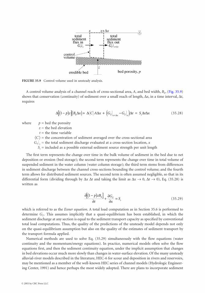
A control volume analysis of a channel reach of cross-sectional area, A, and bed width, Bb, (Fig. 35.9)shows that conservation (continuity) of sediment over a small reach of length, Dx, in a time interval, Dt,requires

(35.28)

where p = bed the porosityz = the bed elevationt = the time variable

·C Ò = the concentration of sediment averaged over the cross-sectional areaGT �x = the total sediment discharge evaluated at a cross-section location, x

Ss = included as a possible external sediment source strength per unit length

The first term represents the change over time in the bulk volume of sediment in the bed due to netdeposition or erosion (bed storage); the second term represents the change over time in total volume ofsuspended sediment in the water column (water column storage); the third term stems from differencesin sediment discharge between the channel cross-sections bounding the control volume; and the fourthterm allows for distributed sediment sources. The second term is often assumed negligible, so that in itsdifferential form (dividing through by Dx Dt and taking the limit as Dx Æ 0, Dt Æ 0), Eq. (35.28) iswritten as

(35.29)

which is referred to as the Exner equation. A total load computation as in Section 35.6 is performed todetermine GT. This assumes implicitly that a quasi-equilibrium has been established, in which thesediment discharge at any section is equal to the sediment transport capacity as specified by conventionaltotal load computations. Thus, the quality of the predictions of the unsteady model depends not onlyon the quasi-equilibrium assumption but also on the quality of the estimates of sediment transport bythe transport formula applied.

Numerical methods are used to solve Eq. (35.29) simultaneously with the flow equations (watercontinuity and the momentum/energy equations). In practice, numerical models often solve the flowequations first, and then the sediment continuity equation, under the implicit assumption that changesin bed elevations occur much more slowly than changes in water-surface elevation. Of the many unsteadyalluvial-river models described in the literature, HEC-6 for scour and deposition in rivers and reservoirs,may be mentioned as a member of the well-known HEC series of channel models (Hydrologic Engineer-ing Center, 1991) and hence perhaps the most widely adopted. There are plans to incorporate sediment

FIGURE 35.9 Control volume used in unsteady analysis.

D D D D D D DD

1 -( )[ ]( ) + + -( ) =+

p z B x C A x G G t S t xb T x x T x s

∂ -( )[ ]∂

+ ∂∂

=1 p zB

t

G

xSb T

s



transport capabilities to the new generation of HEC software, HEC-RAS, but as of this writing, this hasnot yet been performed. An early evaluation (Comm. on Hydrodynamic Models for Flood InsuranceStudies, 1983) of several models, including HEC-6, noted the following general deficiences: unreliableformulation and/or inadequate understanding of sediment-transport capacity, of flow resistance, ofarmoring (see below), and of bank erosion. In spite of the intervening years, this evaluation may still betaken as a cautionary note in using such models.

Effects of a Nonuniform Size Distribution

Natural sediments exhibit a size distribution (also termed gradation), and, since the grain diameterprofoundly influences transport, the effects of size distribution are likely substantial. The crudest modelsof such effects incorporate distribution parameters, such as the geometric standard deviation, sg, inempirical formulae, e.g., the Brownlie formulae. An alternative approach more appropriate for computermodeling divides the distribution into a finite number of discrete size classes. Each size class is charac-terized by a single grain diameter, and results such as the Shields curve or the Rouse equation are appliedto each separate size class, where they are presumably more valid. Total transport is then determined bya summation of the transport in each size class.

The heterogeneous bed material, which constitutes a source or sink of grains of different size classes,must be taken into account. Conventional bed load or total load transport equations or even initiationof motion criteria may not necessarily apply to individual size classes in a mixture. The transport orentrainment into suspension of one size class may influence transport or entrainment of other size classes,so individual size classes may not be treated independently of each other. This is often handled by theuse of empirical ‘hiding’ coefficients. Finer bed material may under erosive conditions be preferentiallyentrained into the flow, with the result that the remaining bed material becomes coarser. This will reducethe rate of erosion relative to the case where the bed consists of uniformly sized fine material. If theavailable fine material is eventually depleted, suspended load transport will be reduced or in the limitentirely suppressed. Eventually, a layer of coarse material termed the armor layer consisting of materialthat is not erodible under the given flow condition may develop, which protects or ‘armors’ the finermaterial below it from erosion, thereby substantially reducing sediment transport and local scour. Armor-ing may also have consequences for flow resistance, since size distribution characteristics of the bed willvary with varying bed shear stress, and hence affect bed roughness and bed forms. In this way, episodichigh-transport events such as floods may have an enduring impact on sediment transport as well as flowdepths. Various detailed numerical models of the armoring process have been developed, and the readeris directed to the literature for further information (Borah et al., 1982; Sutherland, 1987; Andrews andParker, 1987; Holly and Rahuel, 1990a, b; Hydrological Engineering Center, 1991).

Gravel-Bed Streams

Channels in which the bed material consists primarily of coarse material in the gravel and larger rangeare typically situated in upland mountain regions with high bed slopes (S > 0.005), in contrast to sand-bed channels, which are found on flatter slopes of lower lying regions. The same basic concepts summa-rized in previous sections apply also to gravel-bed streams, but the possibly very wide range of grainsizes introduces particular difficulties. Bedforms such as dunes play less of a role, and so grain resistancecan often be assumed dominant; hence an upper regime stage-discharge relationship can be applied. Theeffects of large-scale roughness elements such as cobbles and boulders that may even protrude throughthe water surface may however not be well described by formulae based primarily on data from sand-bed channels. Instead of a gradually varying bed elevation, riffle-pool (or step-pool) sequences of alter-nating shallow and deep flow regions may occur. The wide size range results in transport events thatmay be highly non-uniform across the stream, and highly unsteady in the sense of being dominated byepisodic events. Armoring may also need to be considered. The coarse grain sizes increase the relativeimportance of bedload transport. The highly non-uniform and unsteady nature of the transport hinders



reliable field measurements. Much debate has surrounded the topic of appropriate sampling of the bedsurface material to characterize the grain size distribution. The traditional grid method of Wolman (1954)draws a regular grid over the bed of the chosen reach, with the gravel (cobble or boulder) found at eachof gridpoint being included in the sample.

A friction law proposed specifically for mountain streams is that of Bathurst (1985) based on datafrom English streams (60 mm < d50 < 343 mm, 0.0045 < S < 0.037, 0.3 m3/s < Q < 195 m3/s) for whichthe friction factor, f, is given by

(35.30)

with a reported uncertainty of ±30%. An earlier formula due to Limerinos (1970) is identical in formexcept that Rh is used instead of the depth, H, and Manning’s n is sought rather than f :

(35.31)

KM is the dimensional constant associated with Manning’s equation (see chapter on Open ChannelHydraulics). Using laboratory and field data, Bathurst et al. (1987) assessed various criteria for theinitiation of motion and bedload discharge formulae (including the Meyer-Peter-Muller formula,Eq. [35.18]). They recommended a modified Schoklisch formula for larger rivers (Q > 50 m3/s) wheresediment supply is not a constraint:

(35.32)

where the critical unit-width discharge, qc, is given by

(35.33)

Here, (qs)b is the volumetric unit width bedload discharge, and the units are metric in both equations.These gravel-bed formulae, while representative, are not necessarily the best for all problems; and theyshould be applied with caution and a dose of skepticism.

Defining Terms

Aggradation — Long-term increase in bed-level over an extended reach due to sediment depositionArmoring — A phenomenon in which a layer of coarser particles that are non-erodible under the given

flow condition protects the underlying layer of finer erodible particlesBed forms — Features on an erodible channel bed which depart from a plane bed, e.g., dunes or ripplesBed load — That part of the total sediment discharge which is transported primarily very close to the bedCritical shear stress — The bed shear stress above which general sediment transport is said to beginCritical velocity — The mean velocity above which general sediment transport is said to beginLocal scour — Erosion occurring over a region of limited extent due to local flow conditions, such as

may be caused by the presence of hydraulic structuresSediment discharge — The downstream mass or weight flux of sedimentSuspended load — That part of the total sediment discharge which is transported primarily in suspension

85 62 410

84f

H

d= +. log

K

g

R

n f

R

dM h h

1 6

1084

85 7 3 4

/

. log .= = +

qs

S q qs b f c( ) = -( )2 5 3 2.

qgd

Scf

= 0 21 163

1 1. .



References

Anderson, A.G. (1973). Tentative design procedure for Riprap-lined channels – field evaluation, ProjectRept. 146, St. Anthony Falls Hydraulic Laboratory, University of Minnesota.

Andrews, E.D. and Parker, G. (1987). “Formation of a coarse surface layer as the response to gravelmobility,” in Sediment Transport in Gravel-Bed Rivers, C. R. Thorne, J. C. Bathurst, and R.D. Hey,Eds., Wiley-Interscience, Chichester.

ASCE Sedimentation Engineering (1975), Manuals and Reports on Engineering Practice, No. 54, V. A.Vanoni, Ed., ASCE, New York.

Bathurst, J. C. (1985). “Flow Resistance Estimation in Mountain Rivers,” J. Hydraulic Eng., 111, No. 4,pp. 625–643.

Bathurst, J. C. (1987). “Bed load discharge equations for steep mountain rivers,” in Sediment Transport inGravel-Bed Rivers, C. R. Thorne, J. C. Bathurst, and R.D. Hey, Eds., Wiley-Interscience, Chichester.

Borah, D.K., Alonso, C.V., and Prasad, S.N. (1982). “Routing Graded Sediment in Streams: Formulations,”J. Hydraulics Div., ASCE, 108, HY12, p. 1486–1503.

Brownlie, W.R. (1981). Prediction of Flow Depth and Sediment Discharge in Open Channels, Rept. KH-R-43A, W.M. Keck Lab. Hydraulics and Water Resources, Calif. Inst. Tech., Pasadena, Calif.

Brownlie, W.R. (1983). “Flow Depth in Sand-Bed Channels,” J. Hydraulic Eng. 109, No. 7, p. 959–990.Chang, H.H. (1988). Fluvial Processes in River Engineering, John Wiley & Sons, New York.Committee on Hydrodynamic Models for Flood Insurance Studies (1983). An Evaluation of Flood-Level

Prediction Using Alluvial-River Models, National Academy Press, Washington, D.C.Dawdy, D.R. (1961). “Depth-Discharge Relations of Alluvial Streams,” Water-Supply Paper 1498-C, U.S.

Geological Survey, Washington, D.C.Engelund, F. and Hansen, E. (1967). A Monograph on Sediment Transport in Alluvial Streams, Tekniske

Vorlag, Copenhagen, Denmark.Holly, F.M. Jr. and Rahuel, J.-L. (1990a). “New numerical/physical framework for mobile-bed modeling,

Part 1: Numerical and physical principles,” J. Hydraulic Research, 28, No. 4, p. 401–416.Holly, F.M. Jr. and Rahuel, J.-L. (1990b). “New numerical/physical framework for mobile-bed modeling,

Part 1: Test applications,” J. Hydraulic Research, 28, No. 5, p. 545–563.Hubbell, D.W. (1987). “Bed load sampling and analysis,” in Sediment Transport in Gravel-Bed Rivers, C. R.

Thorne, J. C. Bathurst, and R.D. Hey, Eds., Wiley-Interscience, Chichester.Hydrologic Engineering Center (1991). HEC-6: Scour and Deposition in Rivers and Reservoir, U.S. Army

Corps of Engineers, Davis, CA.Interagency Committee (1957). “Some Fundamentals of Particle Size Analysis, A Study of Methods Used

in Measurement and Analysis of Sediment Loads in Streams,” Report No. 12, Subcommittee onSedimentation, Interagency Committee on Water Resources, St. Anthony Falls Hydraulic Labora-tory, Minneapolis, Minnesota.

Limerinos, J. T. (1970). “Determination of the Manning coefficient from Measured Bed Roughness inNatural Channels,” Water-Supply Paper 1989-B, U.S. Geological Survey, Washington, D.C.

Lyn, D.A. (1993). “Turbulence measurements in open-channel flows over artificial bed forms,” J. HydraulicEng., 119, No. 3, p. 306–326.

Mehta, A.J., Hayter, E.J., Parker, W.R., Krone, R.B., and Teeter, A.M. (1989). “Cohesive Sediment Trans-port. I: Process Description,” J. Hydraulic Eng., 115, No. 8, Aug., p. 1076–1093.

Mehta, A.J., McAnally, W.H., Hayter, E.J., Teeter, A.M., Schoellhammer, D., Heltzel, S.B. and Carey, W.P.(1989). “Cohesive Sediment Transport. II: Application,” J. Hydraulic Eng., 115, No. 8, Aug.,p. 1094–1112.

Neill, C.R. (1967). “Mean Velocity Criterion for Scour of Coarse Uniform Bed Material,” Proc. 12thCongress Int. Assoc. Hydraulic Research, Fort Collins, Colorado, p. 46–54.

Raudkivi, A.J. (1990). Loose Boundary Hydraulics, 3rd ed., Pergamon Press, New York.Richardson, E.V. and Davis, S.R. (1995). Evaluating scour at bridges, FHWA Rept. HEC-18, U.S. Dept. of

Transportation, Federal Highway Administration, Washington, D.C.



Sutherland, A.J. (1987). “Static armour layers by selective erosion,” in Sediment Transport in Gravel-BedRivers, C. R. Thorne, J. C. Bathurst, and R.D. Hey, Eds., Wiley-Interscience, Chichester.

Taylor, B.D. and Vanoni, V.A. (1972). “Temperature Effects in Low-Transport, Flat-Bed Flows,”J. Hydraulics Div., ASCE, 97, HY8, p. 1427–1445.

U.S. Army Corps of Engineers (1995). Hydraulic Design of Flood Control Channel, Technical Engineeringand Design Guides No. 10, EM1110–2–1601, American Society of Civil Engineers, Washington D.C.

van Rijn, L. (1984a). “Sediment Transport, Part 1: Bed Load Transport,” J. Hydraulic Eng., 110, No. 10,p. 1431–1456.

van Rijn, L. (1984b). “Sediment Transport, Part 2: Suspended Load Transport,” J. Hydraulic Eng., 110,No. 11, p. 1613–1641.

Wolman, M.G. (1954) “The Natural Channel of Brandywine Creek, Pennsylvania,” Prof. Paper 271, U.S.Geological Survey, Washington, D.C.

Further Information

Several general books or book chapters on various aspects of sediment transport are available:

1. ASCE Sedimentation Engineering, V. A. Vanoni, Ed., (1975), ASCE Manual No. 54 is a standardcomprehensive account, with very broad coverage of topics related to sediment transport. A newASCE manual, covering topics of more recent interest, is due out shortly.

2. Fluvial Processes in River Engineering, H. H. Chang (1988), Prentice-Hall, Englewood Cliffs, NJ.3. Loose Boundary Hydraulics, 3rd ed., A. J. Raudkivi (1990), Pergamon Press, New York.4. Sediment Transport Technology, D. B. Simons and F. Sentürk (1992), rev. ed., Water Resources

Publications.5. Sediment Transport Theory and Practice, C. T. Yang (1996), McGraw-Hill, New York.6. “Sedimentation and Erosion Hydraulics,” M. H. Garcia, Chap. 6, in Hydraulic Design Handbook,

Larry W. Mays, Ed., (1999), McGraw-Hill, New York.

Special topics are dealt with in

1. Scouring, H. N. C. Breusers and A. J. Raudkivi (1991), Balkema, discusses a variety of problemsinvolving scour.

2. Highways in the River Environment, E. V. Richardson, D. B. Simons, and P. Y. Julien (1990), FHWA-HI-90–016, and Evaluating Scour at Bridges, HEC-18, E. V. Richardson and S. R. Davis (1995), aredocuments produced for the U.S. Federal Highway Administration, and discuss in great detailhydraulic considerations in the design and siting of bridges, including scour, and the recommendeddesign practice in the U.S.

3. Sediment Transport in Gravel-Bed Rivers, C. R. Thorne, J. C. Bathurst, and R. D. Hey, Eds., (1987)John Wiley & Sons, New York, provides information on problems in gravel-bed streams.

4. Sedimentation: Exclusion and Removal of Sediment from Diverted Water, A. J. Raudkivi (1993),Balkema, discusses settling basins and sediment traps.

5. Reservoir Sedimentation Handbook, G. L. Morris and J. Fan, McGraw-Hill, New York, presents anexhaustive discussion of sedimentation in reservoirs.

6. Field Methods for Measurement of Fluvial Sediment, H. P. Guy and V. W. Norman (1970) in theseries Techniques of Water-Resources Investigations of the United States Geological Survey, Book 3,Chap. C2, gives practical advice regarding field measurements of sediment transport, includingsite selection and sampling methods.


Chapter 35: Sediment Transport in Open Channels - Freefreeit.free.fr/The Civil Engineering...

Documents

Transcript of Chapter 35: Sediment Transport in Open Channels - Freefreeit.free.fr/The Civil Engineering...