CHAPTER 3 Surge propagation in multiconductor … 3 Surge propagation in multiconductor transmission...

CHAPTER 3

Surge propagation in multiconductor transmission lines below ground

Nelson Theethayi & Rajeev ThottappillilDivision for Electricity, Uppsala University, Uppsala, Sweden.

Abstract

Surge propagation in underground systems has been a subject of interest for many power and telecommunication engineers. Any typical buried electrical installa-tion involves cables (power or telecommunication) and grounding systems. The cables could have multiple shields and multiconductor confi guration for the core with either twisted or non-twisted conductors. The grounding conductor system could have counterpoise, rods, grids, etc. Interestingly, all these conductor sys-tems could be modelled as multiconductor transmission line (MTL) systems for the wave propagation studies. In this chapter, we shall see how they can be mod-elled for transmission line analysis using the Telegrapher’s equations as discussed in Chapters 1 and 2. A brief discussion on crosstalk mechanisms will also be given, even though the analysis for crosstalk in MTL systems is similar to that in Chapter 2.

1 Introduction

Before we begin this chapter, it is good to visualize some practical problems that constitute a buried conductor system. In power and railway systems, we have cables used for bulk power transmission and signalling/telecommunica-tion purposes. Every high-voltage power transmission tower has a long running counterpoise wire [1, 2] in the ground connected to the foot of the tower. The main purpose is to divert the lightning stroke current directly to the counter-poise wire. This is particularly important when the potential at the tower top or at the footing is of interest. Moreover, in the substation, there are complex grounding systems, which include counterpoise wires, buried rods and buried grids/meshes. To get a broader insight into the problem, let us take an example

www.witpress.com, ISSN 1755-8336 (on-line) WIT Transactions on State of the Art in Science and Engineering, Vol 29, © 2008 WIT Press

doi:10.2495/978-1-84564-063-7/03

80 Electromagnetic Field Interaction with Transmission Lines

of a communication system. Lightning strike to communication towers is a usual phenomenon [3]. A schematic diagram showing most of buried conductor systems connected to a communication tower in a communication tower complex is shown in Fig. 1 [3].

In Fig. 1, the tower foundation and building foundation are connected to their respective ring conductors. The ring conductors are provided primarily to mini-mize the danger of step voltage [4]. Besides, the ring conductor relieves the electri-cal stress at the tower foundation reducing chances of damage to the foundation. The earth conductor between the tower and building ring conductors prevents ground surface arcs between tower and building, and reduces lightning currents carried by cable shields by sharing a part of it. The follow-on earth conductor takes a part of the lightning current away from the service cables. The radial conductors around the tower are for reducing the percentage of lightning current dispatched to the building via the tower cables and earth conductors. The radial conductors are benefi cial only if it can substantially reduce the lightning currents dispatched to the building, especially if the distance between the tower and building is long. The length and design of the radial conductors are to be governed by economy and its effi ciency in dissipating lightning currents into the bulk earth. How do we analyse those buried conductor or grounding systems in the event when lightning or switch-ing fault currents are diverted to them? This could benefi t in the design of protec-tion and grounding systems. This chapter will discuss as to how to use transmission line concepts to such problems but, of course, under the limits of transmission line approximations as discussed in Chapter 2.

Figure 1: Schematic diagram of grounding conductors considering the tower and building as separate units (not to scale), adapted from [3].


Surge Propagation in Multiconductor Transmission Lines 81

2 Telegrapher’s or transmission line equations for the buried wires

Underground wires can be either bare (counterpoise – representative of grounding conductors) or insulated (representative of cable shields or unshielded cables). We shall come to the analysis of coupling through shields later. Hence, one has two different systems for study as shown in Fig. 2.

In addition to ground conductivity and ground permittivity, there is also insulation permittivity for the insulated cables. The soil is characterized by its conductivity and permittivity. For insulated wires, we have insulation permittivity additionally. The corresponding per unit length transmission line representation of the above system is shown in Fig. 3 [5–9] and the relevant equations are shown below. For bare conductor,

gb

d ( , )= ( , )

d

V x jZ I x j

x

ww−

(1a)

gb

d ( , )= ( , )

d

I x jY V x j

x

ww−

(1b)

For insulated conductors,

gi

d ( , )= ( + ) ( , )

d

V x jj L Z I x j

x

ww w−

(2a)

gi

gi

d ( , )= ( , )

d +

CYI x jj V x j

x j C Y

ww w

w

−

(2b)

0= ln2

bL

a

m π

(3a)

Figure 2: Bare and insulated conductor systems in the soil under study.



in2=

ln( / )C

b a

eπ

(3b)

The transmission line equations presented here can be extended to the multicon-ductor transmission line (MTL) system of several buried cables or grounding wires similar to the discussions in Chapter 2. In eqns (1) and (2), V and I are the voltage and currents, respectively. In eqn (1), Zgb and Ygb are the ground impedance and ground admittance of the bare conductor(s). In eqn (2), Zgi and Ygi are the ground impedance and admittance of the insulated conductor(s). Hence, in discussions to follow for ground impedance and ground admittance for buried wires, we defi ne Zgu and Ygu, for ground impedance and admittance, respectively, and the subscript ‘u’ is either ‘b’ or ‘i’, as the case may be, for bare or insulated wires. In eqn (2), L and C are the insulation inductance and capacitance, respectively [5], calculated using eqn (3). Lightning fi rst return stroke or switching transients have frequency components ranging from a few tens to a few hundreds of kilohertz and subse-quent lightning return strokes could have frequencies up to a few megahertz [10, 11]. For this reason, we shall investigate the ground impedance behaviour up to 10 MHz, beyond which the validity of transmission line approximation for buried wires could be questionable and will be discussed later.

The current wave equation for insulated wires can be written in a convenient form as in eqn (4) so that the total shunt element, i.e. series combination of insula-tion capacitance jwC and Ygi in Fig. 3 can be transformed to a parallel combination of insulation capacitance and modifi ed ground admittance, i.e. jwC || Y gi

P , which is

comparable with above-ground wires’ transmission line equations as discussed in Chapter 2, and researchers like [12] have adopted this.

Pgi

d ( , )= ( + ) ( ,

d

I x jj C Y V x j

x

ww w−

(4a)

2P

gigi

( )=

+

j CY

j C Y

ww

−

(4b)

Figure 3: Per unit length transmission line representation for bare and insulated conductor systems in the soil under study.



2.1 Ground impedance for buried wires

In the analysis below, let us assume the radius of the wire as Rab. If the bare wire is in the analysis, then Rab = a else Rab = b, the outer radius of the insulated wire, and the depth of the wire is d. Several researchers have contributed to the development of ground impedance expression for buried wires. The ground impedance expression for buried wires was developed fi rst by Pollaczek [13] in 1926, as shown in eqn (5), which is a low-frequency approximation (similar to that in Chapter 2) in the sense that it can only be used when frequency of incident pulse satisfi es w << sg/eg.

( )( )

20 g

0 ab 0 g

2 2Pollaczek 0 ab 0 g0g

2

20 g

42

ee d

| |ab

d u jju R

K R j

j R d jKZ

uu u j

wm s

wm s

wm wm s

wm s

− ++∞ ⋅−∞

+ ⋅−= π + ⋅ ⋅ + +

∫

(5)

Because of the low-frequency approximation one can see that eqn (5) does not include the permittivity of the ground. All limitations associated with Carson’s ground imped-ance as explained in Chapter 2 for above-ground wires are applicable to Pollaczek’s ground impedance expression for buried wires as well. Saad et al. [14] have analyti-cally showed that an excellent approximation for eqn (5) is given by eqn (6).

( )0 g

0 ab 0 gSaadet al. 0g 2

2ab 0 g

22 e4 ( )

d j

K R jj

Z

R j

wm s

wm swm

wm s− ⋅

+

= π ⋅ +

(6)

Observe that if the infi nite integral, e.g. in eqn (5), is eliminated, then those expres-sions without infi nite integrals we shall here refer to as closed form approxima-tions. Wedepohl and Wilcox [15] and Dommel [16, 17] (who presents expressions of A. Semlyen and A. Ametani) have proposed their own closed form ground impedance expressions, and Saad et al. [14] have shown that those expressions are more or less identical to eqn (6) when numerical calculations were compared.

For a wide range of frequencies, as long as the transmission line approximation is valid, Sunde [6] has derived the ground impedance expression as given by eqn (7). It is similar to eqn (5), but the only difference is that full propagation constant of the soil was used in eqn (7).

( )2 2

g

2 20 ab g 0 g ab

Sunde 02g

ab0 2 2g

( ) 4

e2 2 cos( ) dd u

K R K R d

jZ

uR uu u

g

g gwm

g

− +∞

− + = π + ⋅ ⋅ + +

∫

(7)



The integral term in eqn (7) converges slowly leading to longer computation times and possible truncation errors as the frequency is increased. Further, it was found that the fi rst two Bessel terms in eqn (7) are oscillatory, when frequency is high. However, one can say Sunde’s expression for ground impedance is more valid than Pollaczek’s ground impedance expression in the sense that it uses the full expressions for propa-gation constant. Recently, Bridges [8], Wait [9] and Chen [18] have independently proposed more complex ground impedance expressions derived from rigorous electro-magnetic theory, and in [8, 18] closed form logarithmic approximations for transmis-sion line solution have been proposed. The authors found that even those expressions in appearance, though simple, are oscillatory (perhaps numerical convergence prob-lems) at high frequency, hence not discussed here as it needs further investigation.

Bridges [8] mentions that his complete expression for ground impedance has two modes, namely transmission line modes and radiation/and surface wave modes. Moreover, the solution of his ground impedance expressions is based on complex integration theory and adds that pole term in his expression corresponds to trans-mission line mode and the branch cut corresponds to radiation/and surface wave modes [8]. Thus, under the transmission line modes, it can be shown that Bridges’s expression is identical to Sunde’s expression. Further, Wait [9] proposed a quasi-static approximation (under transmission line modes) and is given by eqn (8).

Wait 0g

ab

1.12= (1+ ) ln

2

j jZ

R

wmk

−Θ π

(8a)

2

g 0 0 g= jk e m w wm s−

(8b)

2 j dV k= (8c)

0 1 2

0 ab

1 2 2= ( ) + ( ) (1+ )e

( )K K

K j RVV V V

k V V−

Θ −

(8d)

Vance [7] proposed one of the simplest closed form approximations for eqn (7) given by eqn (9), where Henkel functions are used instead of Bessel’s functions.

10 ab gVance 0

g 1ab g 1 ab g

( )=

2 ( )

H jRZ

R H jR

gm wg gπ

(9)

Petrache et al. [12] have proposed a logarithmic approximation as shown in eqn (10) for the ground impedance and also claim that it’s the simplest expressions for the ground impedance.

g abLog 0g

g ab

1+= ln

2

RjZ

R

gwmg

π

(10)

It can be seen in eqns (9) and (10) the depth of the wire is missing. Models that neglect air–earth interface [7] are known as infi nite earth models. Wait [9] has



shown that this condition exists if 2g 0 0 g|2 | 1jd je m w wm s− >> . From this condi-

tion, it was found that neglecting the wire depth might not be a good approxima-tion for higher frequencies typical for lightning. Moreover, it was found that for any combination of ground material property, the logarithmic approximation (10) and Vance’s approximation (9) for the ground impedance are identical.

Theethayi et al. [19] proposed a modifi ed empirical logarithmic-exponential approximation (11), which is similar to eqn (9) but with an extra term accounting for wire depth taken from Saad et al. expression (6).

gg ab 2 | |Log-Exp 0g 2 2

g ab ab g

1+ 2= ln + e

2 4 +

dRjZ

R R

ggwmg g

− π

(11)

Note that, in all the expressions above for the mutual impedance between the wires Rab needs to be replaced by horizontal distance between the buried wires and d by average depth [15].

Figures 4 and 5 show the comparison of various ground impedance expressions and the deviations between expressions can be seen clearly both in amplitude and argument responses. The example is a wire of radius 2 cm and a depth of 0.5 m.

Figure 4: Amplitude, |Zg/jw| for comparing eqns (6)–(11): ground conductivity is sg = 1 mS/m and erg = 10.



The consequence of missing depth term in logarithmic expression can be seen in the amplitude, and the consequence of low-frequency approximation in argument response. It can be seen that empirical logarithmic-exponential approximation has some agreement with either Sunde’s or Wait’s expression.

2.1.1 Asymptotic analysisNow let us see the asymptotic behaviour of the ground impedance for buried wires as frequency tends to infi nity (even though such an approach is questionable under transmission line limits). For using the time domain analysis, it is necessary to know the value of the ground impedance at t = 0. It is thus necessary to confi rm if at all the ground impedance pose any singularity as the frequency tends to infi n-ity. Similar to overhead wires, as discussed in Chapter 2, the ground impedance in time domain is referred to as transient ground impedance [5, 10], given by inverse Fourier or Laplace transform as, z(t) = F–1[Zg/jw]. The value at t = 0 can be obtained by initial value theorem as ( ) g

0lim = limt

t Zw

z→ →∞

. Vance’s expression (9) can be rewritten as eqn (12).

0 ab g 0 ab gVance 0 0g

ab g 1 ab g 1 ab g ab g

( ) + ( )= =

2 ( ) + ( ) 2

J jR jY jRj jZ

jR J jR jY jR jR

g gm w m wg g g g

Γ

π π

(12)

Figure 5: Argument (radians), ∠(Zg/jw) for comparing eqns (6)–(10): ground con-ductivity is sg = 10 and 0.1 mS/m and erg = 10.



Simplifying eqn (12), we obtain eqn (13) and using the asymptotic expansions given in [20] it can be shown that lim j

w→∞Γ → .

Vance 0 0g

ab g 0 g g

= =2 2 ( + )

j jZ

jR j j

m w m wg m s we

Γ Γπ π

(13)

Thus, under the asymptotic conditions, it can be shown that eqn (13) tends to eqn (14) as frequency approaches infi nity. The same is applicable with the logarithmic expression (10). Further, in the empirical expression, as frequency tends to infi nity the exponential part approaches zero.

Vance 0g

ab g

1lim =

2Z

Rw

me→∞

π

(14)

A similar expression to eqn (14) has been obtained in Chapter 2 for the over-head wires, the only difference was that in eqn (14) the radius of the conductor Rab is to be replaced by the height of the conductor above ground. For wire of radius 2 cm at a depth of 0.5 m, the asymptotic value of ground impedance is 948 Ω/m. The important dimension here is the outer diameter of the conductor. Equation (14) is also applicable for a tubular conductor or for the shield of a cable in contact with the ground. Clearly, a singularity would appear if ground impedance expression corresponding to the low-frequency approximation was used.

2.2 Ground admittance for buried wires

Once we have the ground impedance, it is simple to get the ground admittance term. Vance [7] suggests that ground impedance and ground admittance are related to each other approximately by the propagation constant as in eqn (15). This approximation is valid in the sense that most of the currents return with in the soil because of which the ratio of electric to magnetic fi elds in the ground should be associated with intrinsic impedance of the soil as discussed in Chapter 2.

2g

gg

=YZ

g

(15)

For a wire of radius 2 cm at a depth of 0.5 m, Figs 6 and 7 show both ground impedance and admittance amplitudes and arguments, respectively. The ground admittance appears to be more sensitive to ground conductivity than ground imped-ance. This is unlike overhead wires where the ground impedance is very sensitive to ground conductivity, as discussed in Chapter 2. The interesting feature is that even though the ground impedance has asymptotic value at a very high frequency, the ground admittance monotonically increases and tends to infi nity as the



frequency is increased, i.e. glim Yw→∞

→ ∞ . Thus it is clear that surge or characteris-tic impedance √

___ Z/Y of the buried bare wire will tend to zero at a very high fre-

quency, unlike overhead wires where it tends to a constant value. For buried insulated cables, the insulation permittivity additionally modifi es the behaviour of total series impedance and shunt admittance of the wire. The modifi ed ground admittance for insulated cables in eqn (4b) has an asymptotic value given by eqn (17) as the frequency tends to infi nity even though the ground admittance of bare wire tends to infi nity. The following arguments support this statement. Petrache et al. [12] have also obtained similar expression as eqn (17). A reason why the total shunt admittance in the current wave equation (2b) tends to infi nity as the fre-quency tends to infi nity is that because the ground admittance term Ygi tends to infi nity as frequency tends to infi nity.

2giP

gigi 0 g

0 g

=

+ +

C ZY

CZ

j j

m sm e

w w

−

(16)

Figure 6: Ground impedance and admittance magnitude response for various ground conductivities for a bare wire of radius 2 cm, buried at 0.5 m depth and erg = 10.



2P 0in

gi0 g g

2 1lim

ln( / ) 2Y

b a bw

mem e e→∞

π → π

(17)

Transient simulation packages like Electromagnetic Transients Program (EMTP) [16, 21] ignores ground admittance and uses low-frequency approximation of ground impedance, i.e. neglects ground permittivity for underground cables. For bare wires, one cannot ignore ground admittance at all that is the reason why there are not any models for counterpoises etc., unlike line and cable models in EMTP [16, 21]. The inadequacies of low-frequency approximations for ground impedance have been dis-cussed in the earlier section and also in Chapter 2. To illustrate the importance of ground admittance, let us consider two cases for an insulated wire corresponding to cable trans-mission line representation shown in Fig. 3. Case 1 is with ground admittance and Case 2 without ground admittance, i.e. Ygi → ∞. The line propagation constant for Cases 1 and 2 are given by eqns (18) and (19), respectively in Laplace domain s ⇔ jw.

1/ 2

gi1 gi

gi

= ( + )+

sCYsL Z

sC Yg

(18)

Figure 7: Ground impedance and admittance argument response for various ground conductivities for a bare wire of radius 2 cm, buried at 0.5 m depth and erg = 10.



1/ 2

2 gi= ( + )sL Z sCg (19)

Observe that when Ygi → ∞, then g1 → g2. The system that is being considered is an insulated cable buried at a depth of 0.5 m and having a radius of 2 cm and an insulation thickness of 2 mm. The ground conductivity is 1 mS/m, and the ground relative permittivity is 10, and the insulation relative permittivity is either 2 or 5. The ratio of attenuation factors for Cases 1 and 2, a1/a2, and the velocity ratio of propagation v1/v2 (note velocity is obtained by the ratio w/b, where w is the angu-lar frequency and b is the phase constant calculated independently, which further is the imaginary part of g) are shown in Figs 8 and 9, respectively.

It can be seen from Fig. 8 that the attenuation per meter for Cases 1 and 2 is same only at 100 Hz, and beyond that frequency, attenuation for Case 1 is a few times higher than Case 2. Situation is worse when the insulation permittivity is higher. Incorrect attenuation of currents at various points would predict incorrect rise times for propagating pulses.

Figure 8: Attenuation ratio for Case 1 (Yg included) and Case 2 (Yg neglected) for a wire of radius 2 cm, insulation thickness of 2 mm and buried at 0.5 m depth, erin = 2 or 5, sg = 1 mS/m and erg = 10.



Now consider the velocity ratio as shown in Fig. 9. The velocity of propagating waves is same for Cases 1 and 2 only until 10 kHz. Beyond this point, again, the velocity ratio is increasing, that is underestimation of velocity when ground admit-tance is neglected. Situation is worse when the insulation permittivity is higher. Velocity of waves propagating in Case 2 is much slower than Case 1. The conse-quence of different velocities between Cases 1 and 2 will result different time delays. Case 2 is certain to predict incorrect velocities. Changing velocity with frequency will cause dispersion in the propagating waves. For the above problem, Theethayi et al. [19] have shown the difference in the attenuations and velocities clearly with time domain simulations as well for a typical pulse propagation problem.

3 Possible limits of transmission line approximation for buried wires

The discussions until now are the analysis based on the transmission line theory. Some discussion on the limits of transmission line approximation was made in Chapter 2. A critical reader may wonder as to what the limit of transmission line approximation is for the buried system as well. For this, we shall use the same

Figure 9: Velocity ratio for Case 1 (Yg included) and Case 2 (Yg neglected) for a wire of radius 2 cm, insulation thickness of 2 mm and buried at 0.5 m depth, erin = 2 or 5, sg = 1 mS/m and erg = 10.



philosophies that were used for overhead wires, i.e. using the concept of penetra-tion depth. Assume the wire is buried at a depth of d meters. The penetration depth at which the currents return in the soil can be calculated using the expres-sion given in Chapter 2 and are shown in Fig. 10 (solid lines) for ground relative permittivity of 10. It should be remembered that the discussion here is applicable for infi nite earth model. So if one considers the infi nite depth models, the penetra-tion depth is defi ned not from the surface of the ground but from the surface of the wire because of the axis-symmetric nature of the problem, unlike overhead wires where the depth was measured from the surface of the ground.

For a wire located at a certain depth in the soil, the currents have a return path only in the soil but at various depths depending upon the frequency of the pulse propagating in the wire. Generally, underground wire type systems in the soil will not be at a depth more than 1 or 2 m. As shown in Chapter 2, the penetration depth attains asymptotic value when the frequency is suffi ciently high, which then becomes independent of frequency and is only dependant on the material proper-ties of the soil. Further, the maximum velocity of the waves propagating in the soil is determined by its permittivity [7], i.e. ugmax = 3 × 108/ √

___ erg . The velocity of the

Figure 10: Penetration depth at which the currents return in the soil for buried wires and wavelength in the soil for erg = 10 and for various ground conductivities.



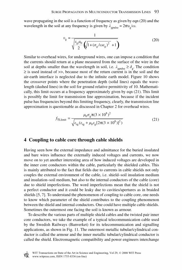
wave propagating in the soil is a function of frequency as given by eqn (20) and the wavelength in the soil at any frequency is given by lgpulse = 2πυg/w.

( )

gg 0 2

g g

1=

1+ ( / ) +12

ue m

s we

(20)

Similar to overhead wires, for underground wires, one can impose a condition that the currents should return at a plane measured from the surface of the wire in the soil at depths smaller than the wavelength in soil, i.e. lgpulse ≥ dg. The condition ≥ is used instead of >>, because most of the return current is in the soil and the air-earth interface is neglected due to the infi nite earth model. Figure 10 shows the crossover points where the penetration depth (solid lines) equals the wave-length (dashed lines) in the soil for ground relative permittivity of 10. Mathemati-cally, this limit occurs at a frequency approximately given by eqn (21). This limit is possibly the limit for transmission line approximation, because if the incident pulse has frequencies beyond this limiting frequency, clearly, the transmission line approximation is questionable as discussed in Chapter 2 for overhead wires.

8 20 g

TLlimit 8 2rg rg 0 g

(3 10 )

( [2 (3 10 )] )f

m s

e e m e

π ×=

+ π ×

(21)

4 Coupling to cable core through cable shields

Having seen how the external impedance and admittance for the buried insulated and bare wires infl uence the externally induced voltages and currents, we now move on to yet another interesting area of how induced voltages are developed in the inner core conductors within the cable, particularly the shielded cables. This is mainly attributed to the fact that fi elds due to currents in cable shields not only couples the external environment of the cable, i.e. shield–soil insulation medium and insulation–soil medium, but also to the internal conductors of the cable (core) due to shield imperfections. The word imperfections mean that the shield is not a perfect conductor and it could be leaky due to cavities/apertures as in braided shields [5, 7]. To understand the phenomenon of coupling to cable core, one needs to know which parameter of the shield contributes to the coupling phenomenon between the shield and internal conductors. One could have multiple cable shields. Sometimes the outermost one facing the soil is known as armour.

To describe the various parts of multiple shield cables and the twisted pair inner core conductors, we take the example of a typical telecommunication cable used by the Swedish Railways (Banverket) for its telecommunication and signalling applications, as shown in Fig. 11. The outermost metallic tubular/cylindrical con-ductor is called the armour and the inner metallic tubular/cylindrical conductor is called the shield. Electromagnetic compatibility and power engineers interchange



the words between armour and outermost shield. Perhaps, for them, armour serves as a mechanical protection for the cable as such. In the coming sections, let us investigate whether an MTL can be derived for multiple shield and multiple core conductors for the transient analysis based on transmission line analysis.

To understand the coupling phenomenon between the tubular/cylindrical con-ductors and the internal conductors, let us start with the concept of transfer imped-ance [5, 7, 22] and later develop expressions for those phenomena in terms of what are known as tube impedances, fi rst introduced by Schelkunoff [22] and later applied by Wedepohl and Wilcox [15]. We extended the analysis of single core cables proposed in [15] to multicore cables, with a view to applying transient analysis of cables with complex internal conductor system. The analysis is based on tubular shields, because it is reasonable to represent the armour and shield of the telecommunication or power cables for frequencies up to several hundreds of kHz as a solid tube. The leakage effects, in authors’ opinion, due to tube apertures and imperfections are predominant only at high frequencies beyond 1 MHz. Under such circumstances, no generalized expressions exist for tube impedances with imperfections and they have to be determined either through experiments or exten-sive theory. A simple/approximate method for determining the capacitance matrix by bridge method is shown and is particularly useful for twisted pair cables appli-cable to most of the telecommunication cables.

Figure 11: A typical telecommunication cable used by the Swedish railways for signalling and telecommunication applications.



4.1 Generalized double shield three-core cable

The discussion presented here is a generalization for a multiconductor arrange-ment of the cable. By using the analogy presented here, one can apply the same to any practical arrangement of the cables. Let us take the following examples: (a) an RG-58 cable that has single core and braided shield – a discussion on the concept of transfer impedance [5, 7] and its experimental determination are presented; (b) three conductor power cables that have a similar shield as that of RG-58 cable. In the authors’ opinion, the analysis of coupling mechanism between the shield and inner conductor as proposed by Vance [7] is valid only for a particular terminal condition. In Vance’s method, when the inner conductor circuit does not carry any appreciable current, the coupling mechanism between the shield and the inner circuit, due to current in the shield, is represented by distributed series voltage sources in the transmission line formed by the inner circuit. This allows us to eliminate the shield circuit and simplify the problem only to a transmission line due to inner circuit. This, in general, is not true for any arbitrary terminal conditions at the near and far ends of the shield and inner conductor/circuit. On the other hand, the analysis presented in the discussions to follow is valid for any arbitrary terminal conditions on either the shield or inner core conductors of the cable.

4.1.1 Telegrapher’s equations for shielded cablesConsider a cable cut away view as shown in Fig. 12, which shows a three-core cable arrangement. It has two shields, solid tubular/cylindrical with annular cross-section. Let the core conductors carry currents I1, I2 and I3. The currents through

Figure 12: Generalized three-conductor cable arrangement for studying the cou-pling between the shields and internal conductors.



the shield and the armour are marked as I4 and I5. In all the cases, let us assume that the external inductance and capacitance matrices are known with the shield as the reference for Fig. 12.

In eqn (22), the voltages V1, V2, V3, V4 and V5 are written in differential form between inner conductors (cores) and the shield, between the shield and the armour and the armour to remote reference, respectively. These voltages are also referred to as loop voltages [15, 16]. The voltages like V1core, V2core, V3core, Vshield and Varmour are that of the conductors with respect to remote reference [15, 16]. These voltages are later useful for a transformation by which one can fi nd voltages on any conduc-tor with respect to any given/specifi ed reference.

1 1core shield=V V V− (22a)

2 2core shield=V V V− (22b)

3 3core shield=V V V− (22c)

4 shield armour=V V V− (22d)

5 armour=V V (22e)

The voltage wave equations based on the loop voltages are given by eqn (23).

111 1 12 2 13 3 14 4 15 5

d= + + + +

d

VZ I Z I Z I Z I Z I

x− ′ ′ ′ ′ ′

(23a)

221 1 22 2 23 3 24 4 25 5

d= + + + +

d


x− ′ ′ ′ ′ ′

(23b)

331 1 32 2 33 3 34 4 35 5

d= + + + +

d


x− ′ ′ ′ ′ ′

(23c)

441 1 42 2 43 3 44 4 45 5

d= + + + +

d


x− ′ ′ ′ ′ ′

(23d)

551 1 52 2 53 3 54 4 55 5

d= + + + +

d


x− ′ ′ ′ ′ ′

(23e)

Since loop voltages are adopted, the currents in eqn (23) are referred to as loop cur-rents I1, I2, I3, I4 and I5. These loop currents are related to the core currents I1core, I2core, I3core, shield current Ishield and armour current Iarmour as shown in eqn (24).

1 1core=I I (24a)

2 2core=I I (24b)

3 3core=I I (24c)



4 shield 1core 2core 3core= + + +I I I I I (24d)

5 armour shield 1core 2core 3core= + + + +I I I I I I (24e)

111 1 12 2 13 3 14 4 15 5

d= + + + +

d

IY V Y V Y V Y V Y V

x− ′ ′ ′ ′ ′

(25a)

221 1 22 2 23 3 24 4 25 5

d= + + + +

d


x− ′ ′ ′ ′ ′

(25b)

331 1 32 2 33 3 34 4 35 5

d= + + + +

d


x− ′ ′ ′ ′ ′

(25c)

441 1 42 2 43 3 44 4 45 5

d= + + + +

d


x− ′ ′ ′ ′ ′

(25d)

551 1 52 2 53 3 54 4 55 5

d= + + + +

d


x− ′ ′ ′ ′ ′

(25e)

The relationship between the conductor currents and loop currents also helps in the transformation by which telegrapher’s equations become in the form similar to MTL systems, as discussed earlier. Now each parameter in the impedance matrix Z' in eqn (23) is a combination of series loop impedances in terms of internal and external impedances. Similarly, each admittance term in Y' in eqn (25) is a com-bination of external and mutual admittance terms forming the loop admittances. These are discussed in Section 4.1.2.

4.1.2 Transmission line impedance and admittance parameters for shielded cables

Our aim is to arrive at the MTL equations of the form eqn (26) after simplifying eqns (22) and (24) using eqns (25) and (23).

1core 1core

2core 2core

3core 3core

shield shield

armour armour

d= [ ]

d

V I

V I

V Z I Xx

V I

V I

−

(26a)

1core 1core

2core 2core

3core 3core

shield shield

armour armour

d= [ ]

d

I V

I V

I Y Vx

I V

I V

−

(26b)



The impedance parameters of eqn (23) are defi ned in eqn (27).

11 i 11 Shield-in= + +Z Z j L Zw′ (27a)

12 21 12 Shield-in= = +Z Z j L Zw′ ′ (27b)

22 i 22 Shield-in= + +Z Z j L Zw′ (27c)

13 31 13 Shield-in= = +Z Z j L Zw′ ′ (27d)

23 32 23 Shield-in= = +Z Z j L Zw′ ′ (27e)

33 33 Shield-in= + +iZ Z j L Zw′ (27f)

14 24 34 41 42 43 Shield-mutual= = = = = =Z Z Z Z Z Z Z−′ ′ ′ ′ ′ ′ (27g)

44 Shield-out Shield-Armour-insulation Armour-in= + +Z Z Z Z′ (27h)

15 25 35 51 52 53= = = = = = 0Z Z Z Z Z Z′ ′ ′ ′ ′ ′ (27i)

45 54 Armour-mutual= =Z Z Z−′ ′ (27j)

55 Armour-out Armour-Earth-insulation g= + +Z Z Z Z′ (27k)

The admittance parameters of eqn (25) are given by eqn (28). Many of the mutual admittance terms are null as shown in eqn (28b), this assumption may not be valid at very high frequencies.

11 12 13 11 12 13

21 22 23 21 22 23

31 32 33 31 32 33

Y Y Y C C C

Y Y Y j C C C

Y Y Y C C C

w′ ′ ′

=′ ′ ′ ′ ′ ′

(28a)

14 15 24 25 34 35

41 51 42 52 43 53

45 54

= = = = = = 0

= = = = = = 0

= = 0

Y Y Y Y Y Y

Y Y Y Y Y Y

Y Y

′ ′ ′ ′ ′ ′ ′ ′ ′ ′ ′ ′ ′ ′

(28b)

44 Sheath-Armour-insulation-capacitance=Y j Cw′

(28c)

55 Armour-Earth-insulation-capacitance g= ||Y j C Yw′

(28d)

In eqn (27), Zi is the internal impedance of the conductors, which is a conseque nce of skin effect phenomena of the core conductors as discussed in Chapter 2. There are some impedance terms in addition to external inductance (discussed later) of the internal conductors in eqn (27). Those impedances, excluding the internal impedances, are the ones that contribute to the coupling between the shield and



inner conductors and the shield and the armour. Let us discuss them in some detail in a while. Insulation capacitance and inductance calculations were explained ear-lier, i.e. using eqn (3). The ground impedance and ground admittance terms appear in eqns (27k) and (28d), which has been discussed in the earlier sections.

If [L]3×3 and [C]3×3 are the inductance and the capacitance matrix of the core conductors with respect to the shield, then for arbitrarily located untwisted con-ductors inside the shield as shown in Fig. 13 (adapted from Paul’s book [23]), those parameters for the core conductors are given by eqns (29) and (30), respec-tively, in the same notations as discussed by Paul [23].

2 2SH G,R0

GG, RRSH wG,R

= ln2

r dL

r r

m − π

(29a)

( ) ( )( ) ( )

2 4 2G R SH G R SH GR0 R

GR 2 4 3SH G R R G R GR

+ 2 cos= ln

2 + 2 cos

d d r d d rdL

r d d d d d

qm

q

− π −

(29b)

For the capacitance matrix as explained in Chapter 2, we fi rst estimate the poten-tial coeffi cient matrix, then invert the potential coeffi cient matrix similar to the above-ground wires. Note that in eqns (30a) and (30b) the permittivity of the insu-lation medium is used.

Figure 13: Untwisted parallel conductor arrangement in the shield for MTL para-meter estimation for multiconductor cables, adapted from [23].



2 2SH G,R

GG,RR0 r SH wG,R

1= ln

2

r dP

r re e

− π

(30a)

2 4 2G R SH G R SH GRR

GR 2 4 30 r SH G R R G R GR

( ) + 2 cos( )1= ln

2 ( ) + 2 cos( )

d d r d d rdP

r d d d d d

qe e q

− π −

(30b)

1= [ ]C P −

(30c)

Schelkunoff [22] gives a very good discussion on the surface impedances of hol-low solid cylindrical shells. Discussions in this section are applicable only for imperfect conductors. Consider a hollow conductor whose inner and outer radii are a and b, respectively. The return of the coaxial path for the current may be provided either outside the given conductor or inside it or partly inside and partly outside. Let Zaa be the surface impedance with internal return and Zbb, with that of external return. This situation has appears to have in effect, two transmission lines with distributed mutual impedance Zab.

According to Schelkunoff, Zab is due to the mingling of two currents in the hollow conductor common to both lines; and since Zab is not the total mutual impedance between the two lines, Zab is called the transfer impedance from one surface of the conductor to the other [22]. Using magnetomotive intensities asso-ciated with the two currents, he derived the surface impedances as given by eqns (31) and (32). The analysis presented here are applicable only to tubular shields.

0 1aa

1 0

( ) ( )=

2 ( ) ( )

I a j K b jjZ

a I b j K a j

wms wmswmss wms wms

+

π Λ

(31a)

0 1bb

1 0

( ) ( ) +=

2 ( ) ( )

I b j K a jjZ

b I a j K b j

wms wmswmss wms wms

π Λ

(31b)

1 1

1 1

( ) ( )=

( ) ( )

I b j K a j

I a j K b j

wms wms

wms wms

− Λ

(31c)

ab ba

1= =

2Z Z

absπ Λ (32)

Two theorems proposed by Schelkunoff [22] with regard to tube impedances are the following.

Theorem 1: If the return path is wholly external (Ia = 0) or wholly internal (Ib = 0), the longitudinal electromotive force (voltage) on that surface which is the nearest to the return path equals the corresponding surface impedance (self) multiplied by



the total current fl owing in the conductor and the longitudinal electromotive force (voltage) on the other surface equals the transfer impedance (mutual) multiplied by the total current.

Theorem 2: If the return path is partly external and partly internal then the total longitudinal electromotive force (voltage) on either side of the surface can be obtained by applying Theorem 1 with the principle of superposition.

Equations (31) and (32) give the tube impedances. In comparison with eqn (27), one can defi ne eqn (31a) as the tube-in impedance of either shield or the armour (31b), as the tube-out impedance of either the shield or the armour, and eqn (32) as the tube-mutual impedance of either the shield or the armour.

Wedepohl and Wilcox [15] have given a very simple approximation as shown in eqns (33) and (34) for the tube impedances without any Bessel functions, and they are valid only if [(b – a)/(b + a)] < 1/8. This has been validated for various practical tubular cable shields by the authors and it was seen that approximations (33) and (34) are excellent ones to exact Schelkunoff equations (31) and (32), respectively.

( )aa

1coth ( )

2 2 ( + )

jZ j b a

a a a b

wmswms

s s≈ − −

π π (33a)

( )bb

1coth ( )

2 2 ( + )

jZ j b a

b b a b

wmswms

s s≈ − −

π π (33b)

( )ab ba

1=

( + ) sinh ( )

jZ Z

a b b a j

wmss wms

≈π −

(34)

It is now shown how to obtain all the important impedance and admittance param-eters that are needed to create the voltage and current wave equations (26a) and (26b).

4.2 An example of RG-58 cable

This cable, based on standard catalogues, has a single core and a braided copper shield. The capacitance of the core conductor with respect to the shield for the RG-58 cable is about 101 pF/m. This can be obtained using the formula (30) if the geometry of the cable is known. The inductance of this cable using the char-acteristic impedance of 50 Ω will be 0.255 µH/m. The shield is braided because of which the tube mutual impedance or the transfer impedance will not be the same as discussed in Section 4.1. Vance [7] mentions that there will be two com-ponents that contribute to the net transfer impedance. One is due to the diffusion of electromagnetic energy across the thickness of the shield and the other, due to



the penetration of the magnetic fi eld through apertures of the braid. The diffusion part is identical to the case as if the shield were like a solid tube, similar to the tube mutual impedance as shown in Section 4.1. The penetration or the leakage part is usually represented as a leakage inductance term as in eqn (35).

Shield-mutual 12= = +T dZ Z Z j Mw (35a)

( )bw

dcbw

2=

sinh 2d

r jZ r

r j

wms

wms

(35b)

The values of Zd and M12 are calculated from the shield geometries and the number of carrier wires on the braid and on the weave angles. The terms rdc and rbw are the dc resistance of the shield and radius of the carrier wire with which the shield is formed. Associated formulas can be found in [7].

Can transfer impedance be measured experimentally? Under the assumption of weak coupling between the inner circuit and the external circuit, it is possible to determine the transfer impedance exactly. Let us get back to our differential equa-tion (23). For the RG-58, the equations reduce to eqns (36) and (37).

core core11 12

21 22shield shield

d=

d

V IZ Z

Z ZV Ix

−

(36)

11 11 12 21 22

12 21 12 22 21 22

22 22

= + + +

= = + = +

=

Z Z Z Z Z

Z Z Z Z Z Z

Z Z

′ ′ ′ ′′ ′ ′ ′

′

(37)

Assume a 1 m length of the RG-58 cable, which is electrically small. At one end (near end marked as suffi x N) let us short the inner conductor and shield, and inject a current source with respect to reference plane. At the other end (far end marked as suffi x F), let us open circuit the inner conductor and short the shield to the refer-ence plane. Thus the voltage at the near and far ends with respect to core and shield currents can be written as

coreF coreN 11 core 12 shield( ) = +V V Z I Z I− − (38a)

shieldF shieldN 21 core 22 shield( ) = +V V Z I Z I− − (38b)

The core current is zero, because of which we have,

coreF coreN 12 shield( ) =V V Z I− − (39a)

shieldF shieldN 22 shield( ) =V V Z I− − (39b)



Also VcoreN and VshieldN are the same as they are shorted at the injection point, hence by subtracting the two equations from each other in eqn (39) we have

coreF shieldF 12 22 shield( ) = ( + )V V Z Z I− −

(40a)

coreF shieldF coreF12 22 12 21

shield shield

( + ) = = =T

V V VZ Z Z Z Z

I I

−− ≈ ≈′ ′

(40b)

This is the concept used in various transfer impedance measurement methods. Similar to transfer impedance, one can also defi ne the transfer admittance. Exper-imentally the Triax set up as shown in Fig. 14 is used for the transfer impedance measurement [24]. There could be other more accurate or simple methods as dis-cussed in [5]. To illustrate the Triax measurements, consider an RG-58 cable of 1 m length and make a simple Triax arrangement [24] as shown in Fig. 14. Note that one can make the radius of the tube smaller so as to be in contact with the outer insulation (not shown in Fig. 14) in order to get rid of the external inductance and capacitance between the tube wall and insulation. Now inject a step pulse current at the near end with the connection as shown in Fig. 14 and measure the open circuit voltage at the far end between the inner core and the shield. The ratio of the open circuit voltage and the shield current should give us the required tube mutual impedance or the transfer impedance.

Assume that for using eqn (35) for the RG-58 cable, the values needed (taken from [7]) are M12 = 1 nH/m, rdc = 14 mΩ/m, rbw = 63.5 µm and the copper conduc-tivity and permeability is chosen. The transfer impedance as a function of fre-quency using eqn (35a) for the above values are shown in Fig. 15.

Note that one could also reproduce the curve using the equations correspond-ing to eqns (32) or (34), if the shield thickness or inner and outer radii are known. It is seen that if the shield was tubular of certain thickness, then the transfer

Figure 14: Triax setup for measuring the transfer impedance.



impedance magnitude decays at high frequencies as shown in Fig. 15, when only the diffusion part is considered. However, if the shield was leaky or braided, then the transfer impedance fi rst decreases at high frequency and then increases as shown in Fig. 15 with both diffusion and the leakage part considered. Tesche et al. [5] mention that the transfer impedance increases at high frequency either as µ f or µ √

_ f , perhaps dependant on the type of the shield. Usually the leakage

part is diffi cult to calculate as it depends on number of carrier wires, their optical coverage, weave angle and, more importantly, they are functions of complete elliptic integrals of fi rst and second kinds. There could be other types of shields that are not braided but similar to the ones shown in Fig. 11, for which no formula exists and controlled measurements can only give the transfer impedance. At low frequencies, the transfer impedance is dominated by only DC resistance of the shield. Similar to transfer impedance one could have transfer admittance, but it exists only if the shield is leaky and at high frequency. The transfer admittance is approximately given by eqn (41). In eqn (41), C1 is the capacitance per unit length between the internal conductors and the shield, C2 is the capacitance per unit length between shield and the external current return path and K is a function with complete elliptic integrals and carriers and weave angle, etc. More details can be

Figure 15: Transfer impedance for an RG-58 cable with braided shield, showing the infl uences of leakage and diffusion part.



found in [5, 7]. As a reasonable approximation, transfer admittance is usually neglected.

T 12

12 1 2

Y j C

C C C K

w≈≈

(41)

4.3 Infl uence of shield thickness in the coupling phenomena

Let us now consider as to what would be the infl uence of shield thickness on the transfer impedance characteristics. For simplicity, we shall consider the example of tubular shields with two thicknesses, namely, 127 and 254 µm, made of copper with an arbitrary outer radius of the shield as 1.65 mm. The expressions (32) or (34) can be used for transfer impedance. One would also get the same if the Traix experiments as explained earlier were made and the ratio of open circuit voltage and shield current were determined. The transfer impedances for the two shield thickness are shown in Fig. 16.

The higher the thickness, the less the transfer impedance, as can be clearly seen in Fig. 16. The transfer impedance in frequency domain shown in Fig. 16 is

Figure 16: Transfer impedance for two shield thicknesses assuming a shield to be solid tubular.



vector fi tted [25] using ten poles and the time domain response is shown in Fig. 17. The value of transfer impedance in time domain is large, which is a result of convolution.

An interpretation can be provided to time domain ‘transfer impedance’ presented in Fig. 17. It takes some time for the shield current (magnetic fi eld) to penetrate inside. The time, when the steady low value of transfer impedance is achieved in Fig. 17, is nearly the same as the time at which the steady value of the open circuit voltage is achieved in Fig. 18. Stern [26] has provided a time domain formula as a series expansion for expression (35b). The convergence of such a time domain for-mula depends on shield properties and shield dimensions. Another interesting fea-ture of the transfer impedance is that it predicts the diffusion time [7] required for the development of the internal voltage. The diffusion time constant can be obtained from the shield thickness and shield material properties and is given by eqn (42).

2

s = (shield thickness)t ms (42)

To demonstrate this, let us take the same example of transfer impedance as above. The internal open circuit voltages, which corresponding to the Triax setup, would have been the product of transfer impedance and shield current for two shield thicknesses

Figure 17: Transfer impedance in time domain for two shield thicknesses assum-ing a shield to be solid tubular.



are shown in Fig. 18. Let us assume a step function for injected shield current. It can then be seen that the constant voltage is attained at about times corresponding to dif-fusion time of the shield and those times are marked in Fig. 18. Note that in generat-ing the curves corresponding to Fig. 18, the frequency domain voltage obtained from the product of transfer impedance and step current in frequency domain were Vector fi tted using ten poles. It is readily see that, higher the thickness, the larger the diffu-sion time and the less the internal voltages due to low value of transfer impedance.

4.4 A simple measurement for estimating inductance and capacitance matrix elements for internal conductors of cables

Today, very sensitive, high precision and accurate measurement systems like AC bridges are commercially available for measurement of smaller values of capaci-tance and inductances. Further, there are voltage and current sensors or instru-ments for measuring small currents and voltages. In this section, we discuss some of the methods to evaluate through experiments, the inductance and capacitance matrix elements for the MTL arrangement of conductors in the cable with respect to the shield based on the method proposed in [5]. This is necessary because there

Figure 18: Time domain response of the internal open circuit voltages for two shield thicknesses assuming the shield to be solid tubular.



could be situations where the medium between the core conductors and the shield is not homogenous and, at the same time, one could have twisted pair arrangement. Under such circumstances practical formulae as discussed earlier, i.e. using eqns (29) and (30), no longer applies.

4.4.1 MTL capacitance matrix estimationLet there be a system of n conductors forming an MTL system inside the shield and let the length of the cable be L. Let one of the ends of the cable be referred to as the near end and the other, as the far end. From the transmission line equations, the relationship between the current in the ith conductor and the voltages on the other conductors are related through admittances as follows.

1 1 1 2 1

d= + + +

di

i i n n

IY V Y V Y V

x

(43)

For a source with line length much less than the wavelength, i.e. under weak cou-pling assumptions we can rewrite eqn (43) as

1 1 1 2 1(0) ( ) [ + + + ]i i i i n nI I L Y V Y V Y V L− ≈ (44)

In eqn (43), Ii(0) and Ii(L) represent the current at the near and far ends, respec-tively. Let all the lines at the far end be left open circuited. Then, for any conduc-tor, the current Ii(L) = 0.

Now at the near end, say if we are interested in calculating the self-capacitance of kth conductor, Ckk, then we do the following. Short all the conductors to the shield in the near end except for the kth conductor where a voltage source Vk is connected to the shield. This voltage source injects a current Ik on the kth, conduc-tor which can also be measured. Then based on eqn (44), since all the voltages are zero at the near end excepting on the kth conductor, we will have

( )0 =k kk k kk kI Y V L j C V Lw≈ (45)

If the voltage source frequency, measured current and applied voltage at the near end is known, then the self capacitance Ckk can be calculated.

Similarly, if we measure the short-circuit current in the jth conductor with the same voltage source Vk with respect to the shield at the near end then we will have eqn (46), from which the mutual capacitance Cjk or Ckj can be obtained.

(0) =j jk k jk kI Y V L j C V Lw≈

(46)

4.4.2 MTL inductance matrix estimationSimilar to eqn (43), we can have the voltage and the currents in the conductor related through the impedance parameters as follows:

1 1 1 2 1

d= + + +

di

i i n n

VZ I Z I Z I

x

(47)



For a source with line length much less than the wavelength, i.e. under weak cou-pling assumptions, we can rewrite eqn (47) as

1 1 1 2 1(0) ( ) [ + + + ]i i i i n nV V L Z I Z I Z I L− ≈ (48)

In eqn (43), Vi(0) and Vi(L) represent the voltage at the near and far ends, respec-tively. Let all the lines at the far end be short-circuited to shield. Then, for any conductor, the current Vi(L) = 0.

Now at the near end, say if we are interested in calculating the self-inductance of kth conductor, Lkk, then we do the following. Open-circuit all the conductors in the near end except on the kth conductor, connect a voltage source Vk with respect to the shield, which injects a current Ik on the kth conductor and that is measured. Then based on eqn (48), since all the currents are zero at the near end excepting on the kth conductor, we will have

(0) =k kk k kk kV Z I L j L I Lw≈ (49)

If the voltage source frequency, measured current and applied voltage at the near end is known, then the self-inductance Lkk can be calculated.

Similarly, if we measure the open circuit voltage in the jth conductor with the same voltage source Vk with respect to the shield injecting current Ik on the kth conductor at the near end, then we will have eqn (50), from which the mutual inductance either Ljk or Lkj can be obtained.

(0) =j jk k jk kV Z I L j L I Lw≈

(50)

5 Some additional cases of ground impedance based on wire geometry

5.1 Impedance with wires on the ground

Having known the expressions for ground impedance and admittance for wires above and below ground, it would be interesting to see what would be the expres-sions for the ground impedance for wires on the surface of the ground. This is needed because there are railway systems where cables are sometimes laid beside the tracks either on the ground or in cable trenches. This can be seen in some typical power and communication systems too. Therefore, it is necessary to know the ground impedance expressions for wires on the ground. Sunde [6] has given the expression for ground impedance for the wires on the ground as eqn (51).

Sunde 0gsbi g ab 1 g ab2 2

g ab

= [1 ( )]j

Z R K RR

wmg g

g−

π

(51)



In the above expressions, the Bessel’s function is used. An expression for ground impedance for wires on the ground can be obtained by using the ground impedance expressions for wires below ground, i.e. using eqn (11) with depth d approaching zero.

g abLog 0gsbi 2 2

g ab ab g

1+ 2= ln +

2 4 +

RjZ

R R

gwmg g

π

(52)

What is interesting to note is that there is not any exponential term in eqn (52). It was seen that the logarithmic term corresponds to ground impedance of wires buried at infi nite depth in the soil [7]. The second term in eqn (52) modifi es or corrects the infi nite depth ground impedance model to obtain the ground imped-ance expression for the wires on the surface of the earth. Therefore, the authors refer eqn (52) as modifi ed logarithmic formula. A comparison between the Sunde’s formula (using Bessel function) and the modifi ed logarithmic formula is shown in Fig. 19. The example is a wire of radius 2 cm, ground conductivity is varied from 10 to 0.1 mS/m, and the ground relative permittivity is 10. It is seen

Figure 19: Comparison between Sunde and modifi ed-logarithmic formula for the ground impedance of wires on the surface of the earth.



that eqn (52) is a good approximation for eqn (51) and does not involve Bessel function. It should be remembered that if there are many parallel wires on the ground surface, the mutual ground impedance expressions could be obtained by substituting in eqn (52) the radius of the wire with horizontal distance between the wires, the same analogy as was applicable for the wires below ground. The ground admittance can be obtained using the propagation constant and the relation (15).

5.2 Mutual impedance with one wire above ground and the other below the ground

The mutual ground impedance expressions between an overhead wire and buried wire can be derived from Sunde’s method [6] but it involves infi nite integrals as shown in eqn (53). In eqn (53), dkl is the horizontal distance between above ground and buried conductors. The height of the overhead wire is h and the wire depth is d. The authors feel that simplifi ed expression for eqn (53) in terms of logarithms or exponentials should be derived to avoid infi nite integrals. It is a subject for future study.

( )2 2g+

0gabbi 2 2

0 g

e= cos( )d

+ +

hu d u

kl

jZ d u u

u u

gwm

g

− −∞

π ∫

(53)

6 Some examples

We have seen various expressions for impedance and admittances for the bare and insulated wires. We have also seen how to model the coupling through cable shields. In this section, we take some examples, which will describe the solutions in time or frequency domain and also a practical example of how crosstalk phe-nomena can be minimized using shielded cables.

6.1 Time domain simulation of pulse propagation in bare and insulated wires

When large transient currents or voltages propagate in bare wires or insulated cables there will be non-linear arcing or breakdown mechanisms occurring within the soil or insulation medium. The mechanisms of soil ionization in grounding systems and insulation breakdown in cables are common during power system transients/faults. To include such non-linear effects only time domain solution of transmission line equations helps. An effi cient way of solving numerically lossy transmission line equations in time domain is by using the fi nite difference time domain (FDTD) method with recursive convolutions as discussed in Chapter 2. The only difference is that a vector fi tting [25] of ground admittance in addition to ground impedance is to be made. The discussions presented here can be found in



Theethayi et al. [19] as well. Further, we will have constant term in addition to the exponential terms while fi tting the ground impedance and admittance terms which has to be used in the FDTD equations as discussed in Chapter 2.

As discussed in the beginning of this chapter, the transmission line equations, either eqns (1) or (2), when transformed to time domain will appear as eqn (54).

0

( , ) ( , )+ ( ) d = 0

tV x t I xt

x

tz t t

t∂ ∂

−∂ ∂∫

(54a)

0

( , ) ( , )+ ( ) d = 0

tI x t V xt

x

th t t

t∂ ∂

−∂ ∂∫

(54b)

Note that in eqn (54), the terms z(t) and h(t) are given by eqns (55a) and (55b), respectively.

1 ( )( ) =

Z jt F

j

wz

w−

(55a)

1 ( )( ) =

Y jt F

j

wh

w−

(55b)

Let us assume that eqns (55) or (56), when fi tted with Vector fi tting, say, up to 10 MHz, will give eqns (57) and (58).

0

=1

( ) ( ) + e i

nt

ii

t Cz t Cz az d −≈ ∑

(56a)

0

=1

( ) ( ) + e i

nt

ii

t Cy t Cy bh d −≈ ∑

(56b)

To demonstrate the fi nal time domain expression, let us discuss considering only eqns (54a) and (56a). Substituting eqns (56a) into (54a), we have

( )0

=10

( , ) ( , )+ ( ) + e d = 0i

t nt

ii

V x t I xCz t Cz

xa t t

d t tt

− − ∂ ∂− ∂ ∂

∑∫

(57)

Let us split eqn (57) as

( )0

=10 0

( , ) ( , ) ( , )+ ( ) d + e d = 0i

t t nt

ii

V x t I x I xCz t Cz

xa tt t

d t t tt t

− − ∂ ∂ ∂− ∂ ∂ ∂

∑∫ ∫

(58)



In eqn (58), the second term with a delta function can be written as a convolution given by eqn (59).

0 0

0

( , ) ( , )( ) d = ( )

t I x I xCz t Cz t

t td t t d t

t t∂ ∂

− − ⊗ ∂ ∂∫

(59)

10 0

( , )( ) = ( , )

I xCz t F Cz j I x j

td t w w

t−∂

− ⊗ ∂ (60)

10 0

( , )( , ) =

I x tF Cz j I x j Cz

tw w− ∂

∂ (61)

From eqn (61), it is clear that Cz0 has dimensions similar to line series inductance and term Cy0 to shunt capacitance. Thus, the fi nal set of transmission line equa-tions in time domain for pulse propagation that needs to be solved is given by eqn (62).

( )0

=10

( , ) ( , ) ( , )+ + e d = 0i

t nt

ii

V x t I x t I xCz Cz

x ta t t

tt

− − ∂ ∂ ∂ ∂ ∂ ∂ ∑∫

(62a)

( )0

=10

( , ) ( , ) ( , )+ + e d = 0i

t nt

ii

I x t V x t V xCy Cz

x tb t t

tt

− − ∂ ∂ ∂ ∂ ∂ ∂ ∑∫

(62b)

It is interesting to see that eqn (62) appears similar to the expressions for overhead wires and the solutions to these equations using the FDTD method are straight forward, as discussed in Chapter 2, using the recursive convolution.

To demonstrate the differences one would obtain between the application of the FDTD method to eqn (62) and solutions using direct frequency domain solutions, as discussed in Chapter 2, we take an example of a bare wire 1 km long and buried at a depth of 0.5 m and having a radius of 7.5 mm. A current source having a peak of 1 A with the shape given by I0 (t) = 1.1274 ( e (1×104)t – e (4×105)t ) is injected one end, and the voltage at the injection point, 100, 200, 300, 400 and 500 m from the injection point by two different methods are shown in Fig. 20 for a ground with sg = 1 mS/m and erg = 10. The differences between the two methods are nominal, which could be due to the numerical errors inherent in both the methods.

6.2 A practical crosstalk problem

In Chapter 2, we have seen the crosstalk mechanisms with the MTL conductor system in the presence of fi nitely conducting ground. Here, we shall consider crosstalk to shielded wires based on weak coupling analysis, i.e. the generator wire circuit currents (source) is not infl uenced by the current in the shielded cable.



Note that the analysis to be presented is applicable to electrically short lines as discussed in Chapter 2. Shielded cables are used to protect the signal wires from external interference and also to provide a return path or reference (e.g. the com-mon coaxial cable type RG-58). First, we consider a perfect shield without any direct fi eld penetration inside, and then fi nd out how connecting the shield ends to the ground infl uence the crosstalk (Fig. 21). For simplicity, the ground is assumed to be perfectly conducting. The cable length is assumed to be electrically small so that the circuit analysis is valid. Let us now consider crosstalk to the shielded wire in the set up shown below. This situation is treated in detail by Paul [23].

First consider the capacitive coupling as discussed in Chapter 2. The shield is assumed to be perfect. Therefore, there is no ‘direct’ coupling between the genera-tor wire and the receptor wire. The coupling capacitance between them is a series combination of CGS and CRS (Fig. 22)

RS GS12

RS GS

=+

C CC

C C (63)

Figure 20: Calculated voltages using the transmission line solution and the FDTD method for a bare wire buried at a depth of 0.5 m, 1 km long and radius of 7.5 mm. The ground medium has sg = 1 mS/m and erg = 10.



The near end and far end crosstalk due to capacitive coupling is given by eqn (64).

Cap Cap N FF N 12 2

N F

= =+

R RV V j C I

R Rw

(64)

Where I2 is approximately given by eqn (65) (assuming currents and voltages in the receptor and shield circuit do not infl uence the currents and voltages of the generator circuit, that is, weak coupling with the generator circuit).

g2

g L+

VI

R R≈

(65)

If the screen is connected to the ground at either end, the screen voltage becomes zero everywhere (low-frequency approximation) and the capacitor CRS is shorted out. There is no capacitive crosstalk in this case, V F Cap = V N Cap = 0 when screen is connected to ground at one end or both ends.

Next, we will consider the inductive coupling. The disturbing current in the gen-erator circuit produces a fl ux in the circuit formed by the shield and the ground plane. This fl ux induces a current in the shield which produces a fl ux opposing the original fl ux in the space between the shield and ground plane. That is, the fl ux link-ing with the circuit formed by the receptor wire and the ground plane is also reduced.

Figure 21: Basic model for crosstalk to shielded cable.

Figure 22: Equivalent circuit for capacitive crosstalk to shielded cable.



In electrically small cables, there can be a shield current fl ow only if both ends of the shield are connected to the ground. Therefore, to reduce inductive coupling, both ends of the shield are to be connected to the ground. The equivalent circuit for the inductive coupling of the shielded wire is given in Fig. 23. In Fig. 23,

M• GR – Mutual inductance between the generator circuit and the receptor circuit.M• RS – Mutual inductance between the receptor circuit and the shield circuit.M• GR – Mutual inductance between the generator circuit and the shield circuit.R• S, LS – Resistance and self inductance of the shield.

The direction of the disturbing current is from near end to the far end. It produces a voltage jwMGSI2 in the shield and drives a current IS in the direction shown. In the absence of the shield, the voltage induced by I2 in the inner wire (receptor wire) would have been jwMGRI2. The shield current IS produces a fl ux that opposes the fl ux produced by I2. Therefore, the induced voltage in the receptor wire would be reduced by an amount equal to jwMRSI2. Note that the two voltage sources in the receptor wire oppose each other. In the absence of shield current, IS, the voltage jwMGSI2 = 0. Shield current is given by eqn (66).

GS 2S

S S

=+

j M II

R j L

ww

(66)

The near end inductive crosstalk voltage is given by eqn (67).

IN NN GR 2 RS S

N F

= ( )+

RV j M I M I

R Rw −

(67)

Substituting eqn (66) in eqn (67), we have

2IN N GS RS

N GR 2N F S S

2N S GR GS RS GR S

2N F S S

=+

+ ( ) =

+ +

R M MV j M I

R R R j L

R j R M M M M LI

R R R j L

ww

w

w ww

− +

−

(68)

Figure 23: Equivalent circuit for inductive crosstalk to shielded cable.



Under weak coupling assumptions, the mutual fl ux linking the receptor circuit and the shield circuit is about the same as the mutual fl ux linking the generator circuit and the receptor wire circuit, leading to MGR ≈ MGS. Similarly, the magnetic fl ux in the shield-ground circuit due to shield current is the same as that magnetic fl ux produced by an equal current in the receptor wire leading to Ls ≈ MRS. Applying these two conditions in eqn (68), we get

IN N SN GR 2

N F S S

Crosstalk with Effect ofshield removed the shield

=+ +

R RV j M I

R R R j Lw

w

(69)

In a similar manner, we can fi nd the crosstalk at the far end, as

IN SFF GR 2

N F S S

Crosstalk with Effect ofshield removed the shield

=+ +

RRV j M I

R R R j Lw

w−

(70)

The effect of the shield appears as a multiplying factor (71) on the crosstalk with-out shield, where ts = Ls/Rs is the shield time constant.

S

S S S

1SF = =

+ 1+

R

R j L jw wt (71)

Shielding Factor (SF) can be approximated as

S

SS

S

1 for 1

SF =for 1

R

j L

w

ww

< τ > τ

(72)

For w < 1/ts,

IN NN GR 2

N F

IN FF GR 2

N F

| | =+

| | =+

RV j M I

R R

RV j M I

R R

w

w

−

(73)

That is, inductive crosstalk increases by 20 dB/decade increase in frequency up to about f = 1/2 πts, or Rs = wLs.

For w > 1/ts,

IN N GR SN 2

N F S

IN GR SFF 2

N F S

| | =+

| | =+

R M RV I

R R L

M RRV I

R R L

(74)



Equation (74) is independent of frequency. That is, inductive crosstalk remains constant for f > 1/2 πts.

Total crosstalk is the sum of capacitive and inductive crosstalk. If the shield is grounded, at least one end, the capacitive coupling contribution is zero, and the induc-tive coupling is reduced by the shield only if the shield is grounded at both ends and the frequency of the interfering signal is greater than the shield cut-off frequency.

7 Concluding remarks

In this chapter, we have seen how the transmission line theory can be extended to solve pulse propagation problems in buried conductors, bare as well as insulated. Two of the key concepts for including the effect of fi nitely conducting ground are the ground impedance and ground admittance. After a review of different expres-sions for these two quantities, we have presented a set of new simple expressions that can represent them. These two new expressions do not involve any compli-cated infi nite integrals and hence computationally very effi cient, at the same time retaining the accuracy. It was pointed out that ground admittance is very sensi-tive to ground conductivity, whereas for overhead conductors (chapter 2) it was ground impedance that was sensitive to ground conductivity. The popularly used transient simulation packages like EMTP/ATP ignores ground admittance and the pitfalls of using these programs for the analysis of underground systems have been pointed out. For the given conductivity and permittivity of ground, the fre-quency up to which transmission line methods could be used for buried systems without signifi cant errors is derived. An MTL method for buried shielded cables is presented. This model is capable of calculating the voltages and current devel-oped internal to the cable due to induced external currents in the shield under all possible terminal conditions (short circuit to open circuit). Numerical examples of pulse propagation in buried bare wires and cables have been presented in time domain and discussed.

Acknowledgements

The authors wish to thank F. Rachidi, C.A. Nucci, M. Paolone, V. Cooray and V.A. Rakov for various technical discussions applicable to the present topic. V. Gopinathan is thanked for the editorial assistance for the language.

References

Bewley, L.V., [1] Travelling Waves on Transmission Systems, John Wiley & Sons, Inc., Chapman & Hall, Ltd.: London, 1933.Transmission Line Reference Book 345 kV and Above [2] , Electric Power Research Institute, Fred Weidner and Son Printers Inc., 1975.EMMA Handbook (Elektromagnetisk miljö anvädarhandbok) [3] , Electromag-netic Environment Handbook, Försvarets MaterielVerk (FMV), 2002.



Lee, C.H. & Meliopoulos, A.P.S., Comparison of touch and step voltages [4] between IEEE Std 80 and IEC 479 – 1. IEE Proc. on Generation, Transmis-sion and Distribution, 146(5), pp. 593–601, 1999.Tesche, F.M., Ianoz, M.V. & Karlsson, T., [5] EMC Analysis Methods and Computational Models, John Wiley and Sons Inc.: New York, 1997.Sunde, E.D., [6] Earth Conduction Effects in the Transmission Systems, Van Nostrand, New York, 1949.Vance, E.F., [7] Coupling to Cable Shields, Wiley Interscience: New York, 1978.Bridges, G.E., Fields generated by bare and insulated cables buried in a [8] lossy half-space. IEEE Trans. on Geoscience and Remote Sensing, 30(1), pp. 140–146, 1992.Wait, J.R., Electromagnetic wave propagation along a buried insulated wire. [9] Canadian Journal of Physics, 50, pp. 2402–2409, 1972.Cooray, V. (ed.), [10] The Lightning Flash, IEE power series, IEE: London, 2003.Rakov, V.A. & Uman, M.A., [11] Lightning Physics and Effects, Cambridge University Press: Cambridge, 2003.Petrache, E., Rachidi, F., Paolone, M., Nucci, C.A., Rakov, V.A. & Uman,[12] M.A., Lightning induced disturbances in buried cables – part I: theory. IEEE Trans. on Electromagnetic Compatibility, 47(3), pp. 498–508, 2005.Pollaczek, F., Sur le champ produit par un conducteur simple infi niment [13] long parcouru par un courant alternatif. Revue Gen. Elec., 29, pp. 851–867, 1931.Saad, O., Gaba, G. & Giroux, M., A closed-form approximation for ground [14] return impedance of underground cables. IEEE Trans. on Power Delivery, 11(3), pp. 1536–1545, 1996.Wedepohl, L.M. & Wilcox, D.J., Transient analysis of underground power [15] transmission systems. Proc. IEE, 120, pp. 253–260, 1973.Dommel, H.W., [16] Electromagnetic Transients Program (EMTP Theory Book), Bonneville Power Administration, 1986.Dommel, H.W., Overhead line parameters from handbook formulas and [17] computer programs. IEEE Trans. on Power Apparatus & Systems, PAS-104, pp. 366–372, 1985.Chen, K.C., Transient response of an infi nite wire in a dissipative medium.[18] Interaction Notes on EMP and Related Subjects, ed. C.E. Baum, IN453, 2001.Theethayi, N., Thottappillil, R., Paolone, M., Nucci, C.A. & Rachidi, F., [19] External impedance and admittance of buried horizontal wires for transient studies using transmission line analysis. IEEE Transactions on Dielectric and Electrical Insulation, 14(3), pp. 751-761, 2007.Spiegel, M.R., [20] Mathematical Handbook of Formulas and Tables, Schaum’s outline series, McGraw-Hill Book Company: New York, 1968.Meyer, W.S. & Liu, T., [21] Alternative Transient Program (ATP) Rule Book, ©1987–1992 by Canadian/American EMTP User Group.



Schelkunoff, S.A., The Electromagnetic theory of coaxial transmission lines [22] and cylindrical shields. Bell Systems Technical Journal, 13, pp. 532–579, 1934.Paul, C.R., [23] Introduction to Electromagnetic Compatibility, John Wiley and Sons Inc.: New York, 1992.Tang, H. & Scuka, V., Time-domain study of a shielding cable system with [24] a nonlinear load. IEEE Trans. on Electromagnetic Compatibility, 41(3), pp. 214–220, 1999.Gustavsen, B. & Semlyen, A., Rational approximation of frequency domain [25] responses by vector fi tting. IEEE Trans. on Power Delivery, 14(3), 1999, pp. 1052–1061.Stern, R.B., Time domain calculation of electric fi eld penetration through [26] metallic shields. IEEE Trans. on Electromagnetic Compatibility, 30(3), pp. 307–311, 1988.


CHAPTER 3 Surge propagation in multiconductor … 3 Surge propagation in multiconductor transmission...

Documents

Transcript of CHAPTER 3 Surge propagation in multiconductor … 3 Surge propagation in multiconductor transmission...