Chapter 3

Statistical Process Control

3.1 Introduction

Operations managers are responsible for developing and maintaining the production pro-cesses that deliver quality products and services. Once the production process is operating,it is often necessary to constantly monitor the process to ensure that it functions the wayit was designed. The statistical methods we introduce in this Chapter represent the mostcommonly–used applications of Statistics in Business, Marketing and Management – atany point in time, there are literally thousands of firms applying these methods. In thisChapter, we deal with the subject of Statistical Process Control.

3.2 Process variation

All production processes result in variation; that is, no product is exactly the same asanother. For example, if you weight two boxes of 500 gram breakfast cereal,

• it is unlikely that either of them will weight exactly 500 grams;

• it is unlikely that they will have the same weight.

All products exhibit some degree of variation. This could be

1. Chance variation – caused by a number of randomly occurring events that are part ofthe production process and that cannot be eliminated without changing the process;

2. Assignable variation – caused by specific events or factors that are frequently tem-porary and that can usually be identified and eliminated.

Example

Dulux manufactures paint for indoor and outdoor domestic use; most of its paint is sold in5 litre tins. The cans are filled by an automatic valve that regulates the amount of paintin each can. The designers of the valve acknowledge that there will be some variation inthe amount of paint, even when the valve is working as it was designed to work. This ischance variation. Occasionally, the valve will malfunction, causing the variation in theamount delivered to each can to increase. This increase is the assignable variation.

85

3.2. Process variation 86

The best way to understand what is happening is to consider the volume of paint in eachcan as a random variable. If the only sources of variation are caused by chance, then eachcan’s volume is drawn from identical distributions. That is, each distribution has the sameshape, mean, and standard deviation. Under such circumstances, the production process issaid to be under control. In recognition of the fact that variation in output will occur evenwhen the process is under control and operating properly, most processes are designed sothat their products will fall within designated specification limits or “specs”. For examplethe process that fills the paint cans may be designed so that the cans contain between 4.98and 5.02 litres. Inevitably, some event or combination of factors in a production processwill cause the process distribution to change. When it does, the process is said to be out

of control. There are several possible ways for the process to go out of control. Here is alist of the most commonly occurring possibilities and their likely assignable causes.

• Level shift

This is a change in the mean of the process distribution. Assignable causes includemachine breakdown, new machine and/or operator, or a change the environment.In the paint can example, a temperature or humidity change may affect the densityof the paint, resulting in less paint in each can.

• Instability

This is the name we apply to the process when the standard deviation increases.This may be caused by a machine in need of repair, defective materials, wear oftools, or a poorly trained operator. Suppose, for example, that a part of the valvethat controls the amount of paint wears down; this could cause greater variationthan normal.

• Trend

When there is a slow, steady shift (either up or down) in the process distributionmean, the result is a trend. This is frequently the result of less–than–regular mainte-nance, operator fatigue, residue or dirt build up, or gradual loss of lubricant. If thepaint control valve becomes increasingly clogged, we would expect to see a steadydecrease in the amount of paint delivered.

• Cycle

This is a repeated series of small observations followed by large observations. Likelyassignable causes include environmental changes, worn parts, or operator fatigue.If there are changes in the voltage in the electricity that runs the machines in thepaint cans example, we might see series of overfilled cans and series of underfilledcans.

The key to quality is to detect when the process goes out of control so that we can correctthe malfunction and restore control of the process. The control chart is the statisticalmethod that we use to detect problems.

3.3. Control charts 87

3.3 Control charts

A control chart is a plot of statistics over time. For example, an x̄–chart plots a seriesof sample means taken over a period of time. Each control chart contains a centreline

and control limits. The control limit above the centreline is called the upper control limit

(UCL) and that below the centreline is called the lower control limit (LCL). If, whenthe sample statistics are plotted, all points are randomly distributed between the controllimits, we conclude that the process is under control. If the points are not randomlydistributed between the control limits, we conclude that the process is out of control.

3.3.1 Example: Paint tins

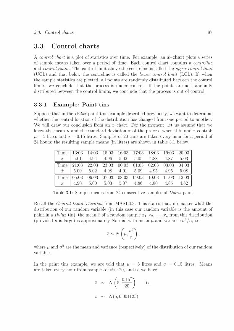
Suppose that in the Dulux paint tins example described previously, we want to determinewhether the central location of the distribution has changed from one period to another.We will draw our conclusion from an x̄–chart. For the moment, let us assume that weknow the mean µ and the standard deviation σ of the process when it is under control;µ = 5 litres and σ = 0.15 litres. Samples of 20 cans are taken every hour for a period of24 hours; the resulting sample means (in litres) are shown in table 3.1 below.

Time 13:03 14:03 15:03 16:03 17:03 18:03 19:03 20:03x̄ 5.01 4.94 4.96 5.02 5.05 4.88 4.87 5.03

Time 21:03 22:03 23:03 00:03 01:03 02:03 03:03 04:03x̄ 5.00 5.02 4.98 4.91 5.09 4.95 4.95 5.08

Time 05:03 06:03 07:03 08:03 09:03 10:03 11:03 12:03x̄ 4.90 5.00 5.03 5.07 4.86 4.80 4.85 4.82

Table 3.1: Sample means from 24 consecutive samples of Dulux paint

Recall the Central Limit Theorem from MAS1403. This states that, no matter what thedistribution of our random variable (in this case our random variable is the amount ofpaint in a Dulux tin), the mean x̄ of a random sample x1, x2, . . . , xn from this distribution(provided n is large) is approximately Normal with mean µ and variance σ2/n, i.e.

x̄ ∼ N

(

µ,σ2

n

)

,

where µ and σ2 are the mean and variance (respectively) of the distribution of our randomvariable.

In the paint tins example, we are told that µ = 5 litres and σ = 0.15 litres. Meansare taken every hour from samples of size 20, and so we have

x̄ ∼ N

(

5,0.152

20

)

i.e.

x̄ ∼ N(5, 0.001125)

3.3. Control charts 88

Also recall from MAS1403 that x̄ ± 1 standard deviation gives about 68% coverage forthe Normal distribution; x̄ ± 2 standard deviations gives about 95% coverage and x̄ ±3 standard deviations gives about 99% coverage. Thus, the lower and upper control limitsfor an x̄–chart are often defined as:

Lower control limit = µ− 3 standard errors = µ− 3

√

σ2

n= µ− 3

σ√n

Upper control limit = µ+ 3 standard errors = µ+ 3

√

σ2

n= µ+ 3

σ√n

For the Dulux paint example, this would give:

Lower control limit = 5− 3×0.15√20

= 4.899 (= 5− 3×√0.001125)

Upper control limit = 5 + 3×0.15√20

= 5.101 (= 5 + 3×√0.001125)

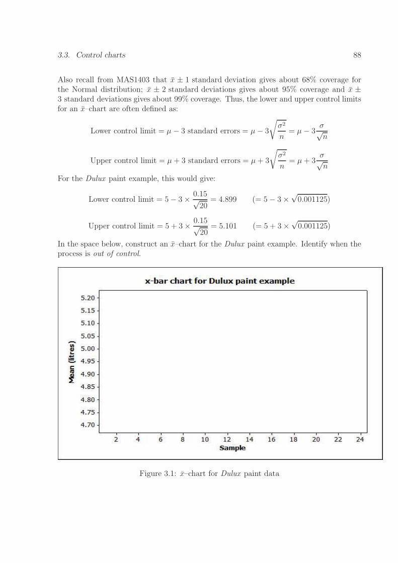
In the space below, construct an x̄–chart for the Dulux paint example. Identify when theprocess is out of control.

Figure 3.1: x̄–chart for Dulux paint data

3.3. Control charts 89

3.3.2 2–sigma and 3–sigma control limits

The control limits we used in the example above are called “3–sigma” control limits, sincewe used a distance of 3 standard errors either side of the mean as a tool to detect theprocess being out of control. Why not use “2–sigma” control limits? Well, sometimesthese are used, although the following reasoning should help explain why 3–sigma controllimits are often preferred.

Suppose we have

H0 : The process is under control

H1 : The process is out of control

In statistical process control, a Type I error occurs if we conclude that the process is outof control when in fact it is not (i.e. reject H0 when in fact it is true). This sort of errorcan be quite expensive: if there is evidence to suggest that the process is out of control,then the production process is usually stopped and the causes of the variation are foundand repaired – stopping the production process is costly, especially if there was no needto do so! So, we would like the probability of a Type I error to be as small as possible.For the paint tins example, we can work out the probability of a Type I error as follows.

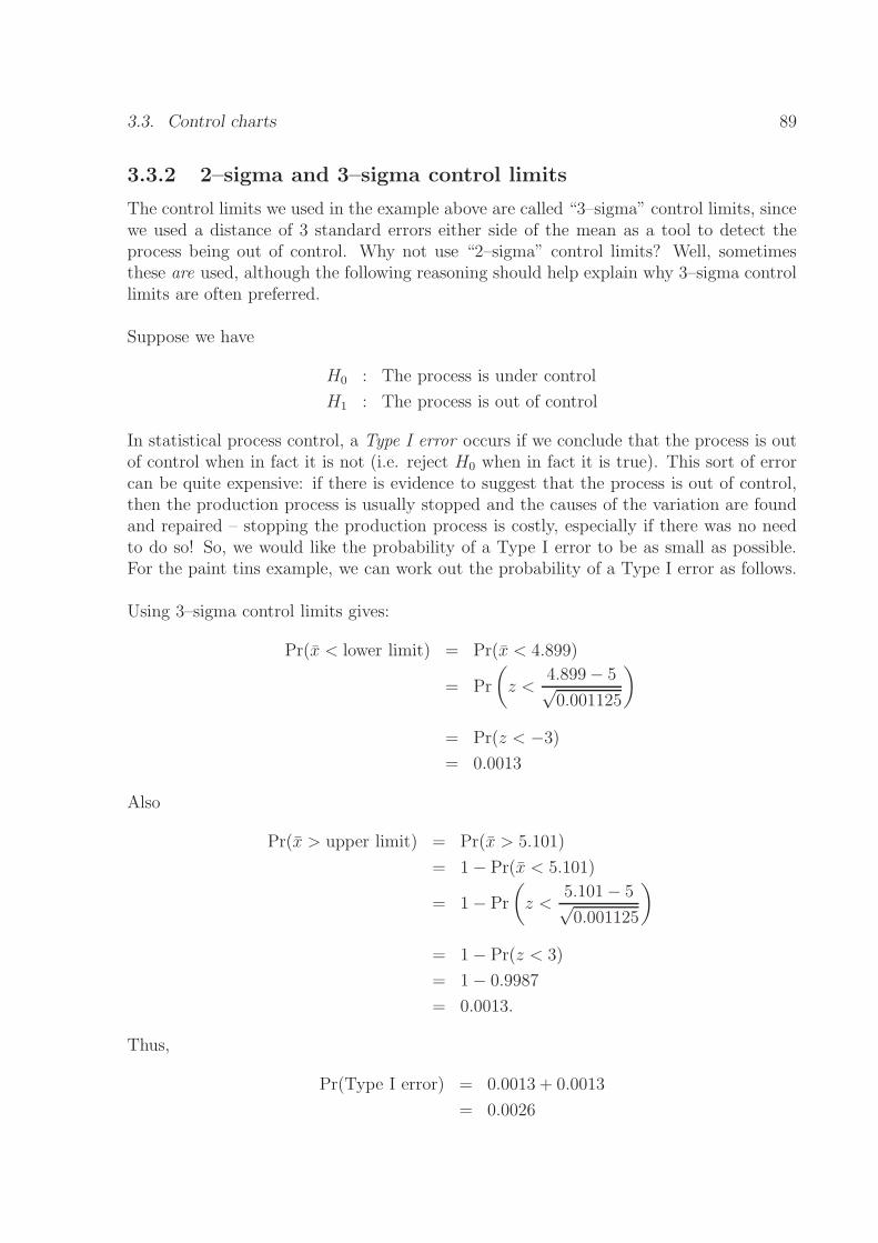
Using 3–sigma control limits gives:

Pr(x̄ < lower limit) = Pr(x̄ < 4.899)

= Pr

(

z <4.899− 5√0.001125

)

= Pr(z < −3)

= 0.0013

Also

Pr(x̄ > upper limit) = Pr(x̄ > 5.101)

= 1− Pr(x̄ < 5.101)

= 1− Pr

(

z <5.101− 5√0.001125

)

= 1− Pr(z < 3)

= 1− 0.9987

= 0.0013.

Thus,

Pr(Type I error) = 0.0013 + 0.0013

= 0.0026

3.3. Control charts 90

Of course, we could have turned to the standard Normal distribution immediately and,owing to the symmetry of the Normal distribution:

Pr(Type I error) = 2× Pr(z < −3)

= 2× 0.0013

= 0.0026.

Similarly, if we use 2–sigma control limits, we would have

Pr(Type I error) = 2× Pr(z < −2)

= 2× 0.0228

= 0.046.

Thus, using 3–sigma control limits will give a false alarm in about 0.26% of samples;using 2–sigma control limits increases this to about 4.6% of samples.

A Type II error occurs when we do not detect when the process is out of control (i.e. weretain H0 when in fact it is false).

3.3.3 Average run length

The average run length (ARL) is the expected number of samples that must be takenbefore the control chart indicates that the process has gone out of control. The ARL isdetermined by

ARL =1

P

where P is the probability that a sample mean falls outside the control limits. Assumingthat 3–sigma control limits are used, this would give

ARL =1

0.0026= 385.

This means that when the process is under control, the x̄–chart will erroneously concludethat it is out of control once every 385 samples, on average. If the sampling plan calls forsamples to be taken once every hour (as in the paint tins example), on average there willbe a false alarm once every 385 hours.

3.3.4 Examples

1. Find the upper and lower 2–sigma control limits for the Dulux paint example. Alsofind the ARL for such a control chart.

3.3. Control charts 91

Lee

2. If the control limits of an x̄–chart are set at 2.5 standard errors from the centreline,what is the probability that on any sample the control chart will give a false alarm?

3.3. Control charts 92

3. A firm manufactures notebook computers. For one component, the company drawssamples of size 10 every half an hour. The company makes 4000 of these componentsevery hour. The control limits of the x̄–chart are set at 3 standard errors from themean. When the process goes out of control, it usually shifts the mean by about0.75 standard deviations.

(a) On average, how many units will be produced until the control chart gives afalse alarm?

(b) Find the probability that the x̄–chart does not detect a shift of 0.75 standarddeviations on the first sample after the shift occurs.

In the examples presented so far, we have assumed that the process parameters (µ andσ) were known. When the parameters are unknown, we estimate their values from thesample data. In the next section, we discuss how to construct and use control charts inmore realistic situations. We will re–visit x̄–charts in section 3.4, as well as S–charts,and we call these control charts for variables. In section 3.5 we will also consider controlcharts for attributes.

3.4. Control charts for variables 93

3.4 Control charts for variables

There are several ways to determine whether a change in the process distribution hasoccurred. To determine whether the distribution means have changed, we employ thex̄–chart. To determine whether the process distribution standard deviation has changed,we can use the S–chart or the R–chart (S for standard deviation, R for range).

3.4.1 x̄–chart

In the previous section we determined the centreline and the control limits of an x̄–chartusing the mean and standard deviation of the process distribution. However, it is unre-alistic to believe that the mean and standard deviation of the process distribution willbe known. Thus, to construct the x̄–chart, we need to estimate the relevant parametersfrom the data.

We begin by drawing samples when we have determined that the process is under control.For each sample, we compute the mean and standard deviation. The estimator of themean of the distribution is the mean of the sample means (denoted ¯̄x and pronounced “xbar bar” or “x double bar”), given by

¯̄x =

∑k

j=1x̄j

k,

where x̄j is the mean of the jth sample and there are k samples. To estimate the standarddeviation of the process distribution, we calculate the “pooled standard deviation”, whichwe denote S and define as

S =

√

∑k

j=1s2j

k.

In the previous section, where we assumed that the process distribution mean and variancewere known, the centreline and control limits were defined as

centreline = µ

Lower control limit = µ− 3σ√n

Upper control limit = µ+ 3σ√n

Because the values of µ and σ are now unknown, we must use the sample data to estimatethem. The estimator of µ is ¯̄x and the estimator of σ is S. Therefore, the centreline andcontrol limits are now:

centreline = ¯̄x

Lower control limit = ¯̄x− 3S√n

Upper control limit = ¯̄x+ 3S√n

3.4. Control charts for variables 94

Example: Car Giant car seats

Car Giant manufactures seats for Mazda and Lexus cars. One of the components of afront seat cushion is a wire spring, produced from 4mm steel wire. A machine is usedto bend the wire so that the spring’s length is 500mm. If the springs are longer than500mm they will loosen and eventually fall out. If they are too short, they won’t easilyfit into position. To determine whether the process is under control, random samples offour springs are taken every hour. The last 25 samples are shown in the table below.

Sample Spring 1 Spring 2 Spring 3 Spring 4 Mean (x̄j) St. dev. (sj)1 501.02 501.65 504.34 501.10 502.027 1.566892 499.80 498.89 499.47 497.90 499.015 0.833093 497.12 498.35 500.34 499.33 498.785 1.375564 500.68 501.39 499.74 500.41 500.555 0.682675 495.87 500.92 498.00 499.44 498.558 2.152036 497.89 499.22 502.10 500.03 499.810 1.763247 497.24 501.04 498.74 503.51 500.132 2.740848 501.22 504.53 499.06 505.37 502.545 2.933819 499.15 501.11 497.96 502.39 500.152 1.9778210 498.90 505.99 500.05 499.33 501.068 3.3157811 497.38 497.80 497.57 500.72 498.368 1.5777112 499.70 500.99 501.35 496.48 499.630 2.2162613 501.44 500.46 502.07 500.50 501.118 0.7799314 498.26 495.54 495.21 501.27 497.570 2.8199615 497.57 497.00 500.32 501.22 499.027 2.0585316 500.95 502.07 500.60 500.44 501.015 0.7348717 499.70 500.56 501.18 502.36 500.950 1.1188718 501.57 502.09 501.18 504.98 502.455 1.7241119 504.20 500.92 500.02 501.71 501.712 1.7963220 498.61 499.63 498.68 501.84 499.690 1.5069421 499.05 501.82 500.67 497.3622 497.85 494.08 501.79 501.9523 501.08 503.12 503.06 503.5624 500.75 501.18 501.09 502.8825 502.03 501.44 498.76 499.39

Table 3.2: Spring data for Car Giant car seats

Complete the table by finding the mean and standard deviation for samples 21–25.

3.4. Control charts for variables 95

The mean of the means – ¯̄x – is given by

¯̄x =502.027 + 499.015 + . . .

25

= 500.296.

Also, the pooled standard deviation S is found as

S =

√

1.566892 + 0.833092 + . . .

25

=

√

97.125

25

= 1.971

Thus, the centreline and control limits are

Centreline = ¯̄x = 500.296

Lower control limit = ¯̄x− 3S√n= 500.296− 3×

1.971√4

= 497.34

Upper control limit = ¯̄x+ 3S√n= 500.296 + 3×

1.971√4

= 503.253

This produces the x̄–chart shown in figure 3.2. Don’t forget – you should be able to produce

these plots by hand! Is the process in control or out of control?

Figure 3.2: x̄–chart for Car Giant springs dataset

As you can probably tell, I produced the plot shown in figure 3.2 using Minitab. To dothis, all the data need to be in a single column, i.e.

3.4. Control charts for variables 96

501.02

501.65

504.34

501.10

499.80

498.89

499.47

497.90

497.12

.

.

.

501.44

498.76

499.39

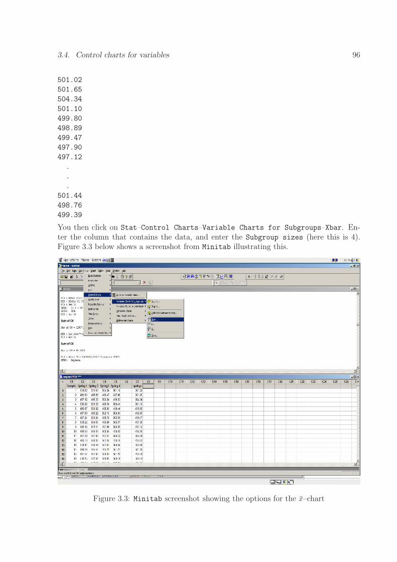
You then click on Stat–Control Charts–Variable Charts for Subgroups–Xbar. En-ter the column that contains the data, and enter the Subgroup sizes (here this is 4).Figure 3.3 below shows a screenshot from Minitab illustrating this.

Figure 3.3: Minitab screenshot showing the options for the x̄–chart

3.4. Control charts for variables 97

3.4.2 S–charts

The S–chart graphs sample standard deviations to determine whether the process distri-bution standard deviation has changed. The format is similar to that of the x̄ chart. TheS chart will display a centreline and control limits. However, the formulae for the cen-treline and control limits are more complicated than those for the x̄–chart; Consequently,we will let Minitab do the work here!

With the data stacked as before (see page 94), we click on Stat–Control Charts–Variables Charts for Subgroups–S; we enter the column with the stacked data, andwe enter the Subgroup sizes as 4. In S options, we need to make sure that the Pooledstandard deviation is selected under Method for estimating standard deviation

within Estimate. Clicking OK gives the plot shown in figure 3.4.

Figure 3.4: S–chart for Car Giant springs dataset

Comments

3.4. Control charts for variables 98

3.4.3 x̄–charts and S–charts in practice: Monitoring the pro-

duction process

In this section, we have introduced x̄–charts and S–charts as separate procedures. Inactual practice, however, the two charts must be drawn and assessed together. Thereason for this is that the x̄–chart uses S to calculate the control limits. Consequently,if the S–chart indicates that the process is out of control, the value of S will not leadto an accurate estimate of the standard deviation of the process distribution. The usualprocedure is:

1. Draw the S–chart first;

2. If this indicates that the process is under control, then draw the x̄–chart;

3. If the x̄–chart also indicates that the process is under control, we can then use bothcharts to maintain control;

4. If either chart shows that the process was out of control at some time during thecreation of the charts, we can detect and fix the problem and then re–draw thecharts with new data.

When the process is under control, we can use the control chart limits and centreline tomonitor the process in the future. We do so by plotting all future statistics on the controlchart.

Example: Back to Car Giant car seats

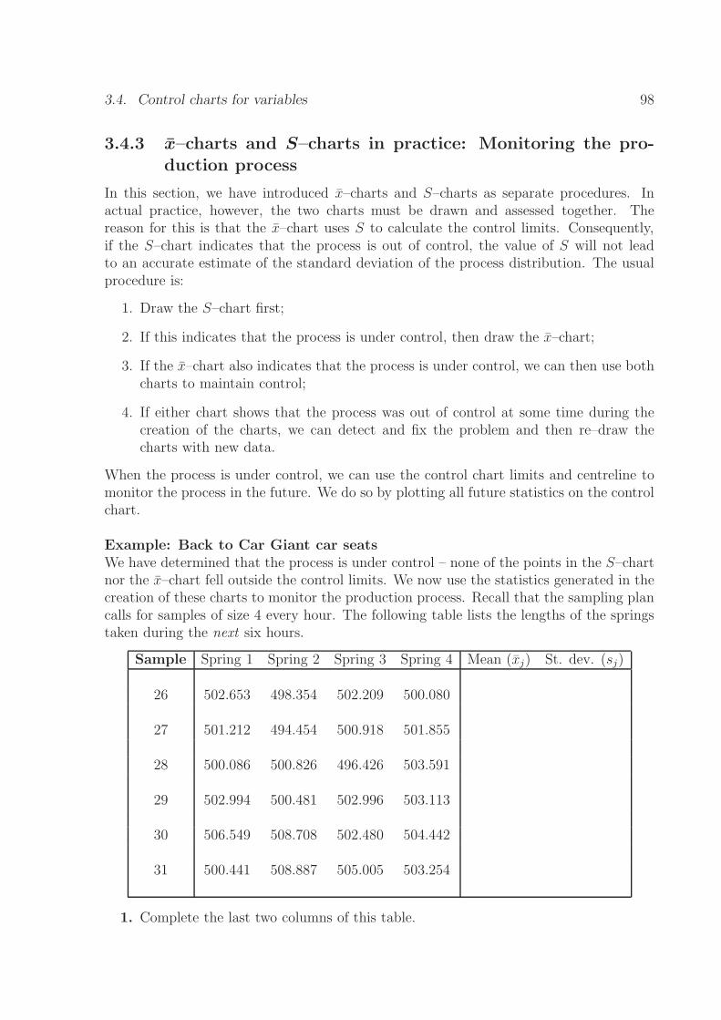
We have determined that the process is under control – none of the points in the S–chartnor the x̄–chart fell outside the control limits. We now use the statistics generated in thecreation of these charts to monitor the production process. Recall that the sampling plancalls for samples of size 4 every hour. The following table lists the lengths of the springstaken during the next six hours.

Sample Spring 1 Spring 2 Spring 3 Spring 4 Mean (x̄j) St. dev. (sj)

26 502.653 498.354 502.209 500.080

27 501.212 494.454 500.918 501.855

28 500.086 500.826 496.426 503.591

29 502.994 500.481 502.996 503.113

30 506.549 508.708 502.480 504.442

31 500.441 508.887 505.005 503.254

1. Complete the last two columns of this table.

3.4. Control charts for variables 99

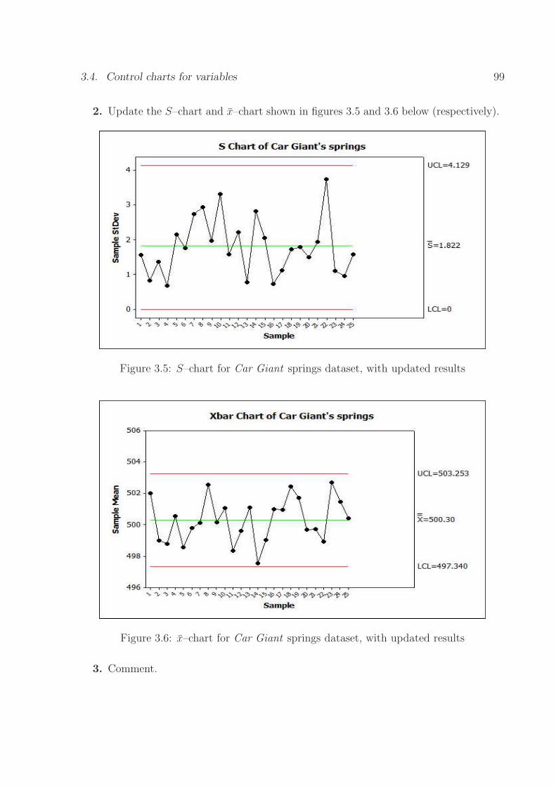
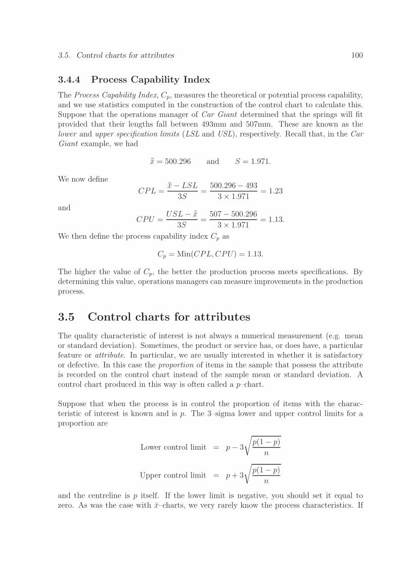
2. Update the S–chart and x̄–chart shown in figures 3.5 and 3.6 below (respectively).

Figure 3.5: S–chart for Car Giant springs dataset, with updated results

Figure 3.6: x̄–chart for Car Giant springs dataset, with updated results

3. Comment.

3.5. Control charts for attributes 100

3.4.4 Process Capability Index

The Process Capability Index, Cp, measures the theoretical or potential process capability,and we use statistics computed in the construction of the control chart to calculate this.Suppose that the operations manager of Car Giant determined that the springs will fitprovided that their lengths fall between 493mm and 507mm. These are known as thelower and upper specification limits (LSL and USL), respectively. Recall that, in the CarGiant example, we had

¯̄x = 500.296 and S = 1.971.

We now define

CPL =¯̄x− LSL

3S=

500.296− 493

3× 1.971= 1.23

and

CPU =USL− ¯̄x

3S=

507− 500.296

3× 1.971= 1.13.

We then define the process capability index Cp as

Cp = Min(CPL,CPU) = 1.13.

The higher the value of Cp, the better the production process meets specifications. Bydetermining this value, operations managers can measure improvements in the productionprocess.

3.5 Control charts for attributes

The quality characteristic of interest is not always a numerical measurement (e.g. meanor standard deviation). Sometimes, the product or service has, or does have, a particularfeature or attribute. In particular, we are usually interested in whether it is satisfactoryor defective. In this case the proportion of items in the sample that possess the attributeis recorded on the control chart instead of the sample mean or standard deviation. Acontrol chart produced in this way is often called a p–chart.

Suppose that when the process is in control the proportion of items with the charac-teristic of interest is known and is p. The 3–sigma lower and upper control limits for aproportion are

Lower control limit = p− 3

√

p(1− p)

n

Upper control limit = p+ 3

√

p(1− p)

n

and the centreline is p itself. If the lower limit is negative, you should set it equal tozero. As was the case with x̄–charts, we very rarely know the process characteristics. If

3.5. Control charts for attributes 101

p is unknown, we estimate it from the data. In the above formulae, we replace p with p̄,where

p̄ =

∑k

j=1p̂j

k,

where p̂j is the sample proportion of items with the attribute of interest in sample j, andthere are k samples in total.

Example

A company that produces USB memory sticks has been receiving complaints from itscustomers about the large number of devices that will not store data properly. Companymanagement has decided to institute statistical process control to remedy the problem.Every hour, a random sample of 200 memory sticks is taken, and each is tested to deter-mine whether it is defective. The number of defective memory sticks in the samples of size200 for the first 40 hours is shown in table 3.3 below. Using these data, draw a p–chart tomonitor the production process. Was the process out of control when the sample resultswere generated?

19 5 16 20 6 12 18 6 13 1510 6 7 10 18 20 13 6 8 38 7 4 19 3 19 9 10 10 1815 16 5 14 3 10 19 13 19 9

Table 3.3: Number of defective memory sticks in 40 consecutive samples of size 200

Outline solution

For each sample we compute the proportion of defective memory sticks, i.e. for sample 1:

p̂1 =19

200= 0.095.

Similarly, for sample 2:

p̂2 =5

200= 0.025.

We then find the mean of all these proportions (p̄), which for the control chart gives

Centreline = p̄ = 0.05762.

The lower and upper control limits are then found as:

Lower control limit = p̄− 3

√

p̄(1− p̄)

n

= 0.05762− 3×√

0.05762× 0.94238

200

= 0.008188 and

3.5. Control charts for attributes 102

Upper control limit = p̄ + 3

√

p̄(1− p̄)

n

= 0.05762 + 3×√

0.05762× 0.94238

200

= 0.1071.

We then produce a plot of the calculated proportions p̂j , along with the centreline andcontrol limits, giving the plot shown in figure 3.7.

Figure 3.7: p–chart for the proportion of defective memory sticks

In Minitab, we would click on Stat–Control Charts–Attributes Charts–P; enter thecolumn with the (stacked) data in in Variables, enter the Subgroup sizes (200 here),and then click OK.

Comments

3.5. Control charts for attributes 103

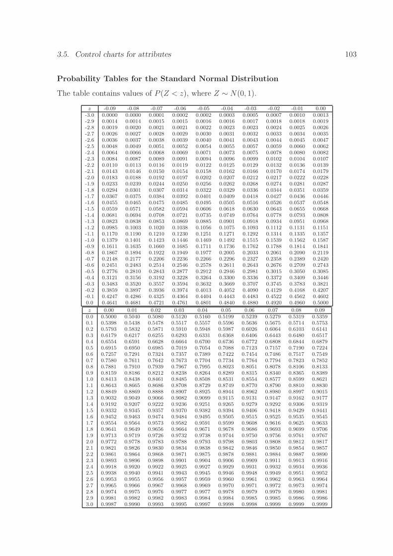
Probability Tables for the Standard Normal Distribution

The table contains values of P (Z < z), where Z ∼ N(0, 1).

z -0.09 -0.08 -0.07 -0.06 -0.05 -0.04 -0.03 -0.02 -0.01 0.00

-3.0 0.0000 0.0000 0.0001 0.0002 0.0002 0.0003 0.0005 0.0007 0.0010 0.0013

-2.9 0.0014 0.0014 0.0015 0.0015 0.0016 0.0016 0.0017 0.0018 0.0018 0.0019

-2.8 0.0019 0.0020 0.0021 0.0021 0.0022 0.0023 0.0023 0.0024 0.0025 0.0026

-2.7 0.0026 0.0027 0.0028 0.0029 0.0030 0.0031 0.0032 0.0033 0.0034 0.0035

-2.6 0.0036 0.0037 0.0038 0.0039 0.0040 0.0041 0.0043 0.0044 0.0045 0.0047

-2.5 0.0048 0.0049 0.0051 0.0052 0.0054 0.0055 0.0057 0.0059 0.0060 0.0062

-2.4 0.0064 0.0066 0.0068 0.0069 0.0071 0.0073 0.0075 0.0078 0.0080 0.0082

-2.3 0.0084 0.0087 0.0089 0.0091 0.0094 0.0096 0.0099 0.0102 0.0104 0.0107

-2.2 0.0110 0.0113 0.0116 0.0119 0.0122 0.0125 0.0129 0.0132 0.0136 0.0139

-2.1 0.0143 0.0146 0.0150 0.0154 0.0158 0.0162 0.0166 0.0170 0.0174 0.0179

-2.0 0.0183 0.0188 0.0192 0.0197 0.0202 0.0207 0.0212 0.0217 0.0222 0.0228

-1.9 0.0233 0.0239 0.0244 0.0250 0.0256 0.0262 0.0268 0.0274 0.0281 0.0287

-1.8 0.0294 0.0301 0.0307 0.0314 0.0322 0.0329 0.0336 0.0344 0.0351 0.0359

-1.7 0.0367 0.0375 0.0384 0.0392 0.0401 0.0409 0.0418 0.0427 0.0436 0.0446

-1.6 0.0455 0.0465 0.0475 0.0485 0.0495 0.0505 0.0516 0.0526 0.0537 0.0548

-1.5 0.0559 0.0571 0.0582 0.0594 0.0606 0.0618 0.0630 0.0643 0.0655 0.0668

-1.4 0.0681 0.0694 0.0708 0.0721 0.0735 0.0749 0.0764 0.0778 0.0793 0.0808

-1.3 0.0823 0.0838 0.0853 0.0869 0.0885 0.0901 0.0918 0.0934 0.0951 0.0968

-1.2 0.0985 0.1003 0.1020 0.1038 0.1056 0.1075 0.1093 0.1112 0.1131 0.1151

-1.1 0.1170 0.1190 0.1210 0.1230 0.1251 0.1271 0.1292 0.1314 0.1335 0.1357

-1.0 0.1379 0.1401 0.1423 0.1446 0.1469 0.1492 0.1515 0.1539 0.1562 0.1587

-0.9 0.1611 0.1635 0.1660 0.1685 0.1711 0.1736 0.1762 0.1788 0.1814 0.1841

-0.8 0.1867 0.1894 0.1922 0.1949 0.1977 0.2005 0.2033 0.2061 0.2090 0.2119

-0.7 0.2148 0.2177 0.2206 0.2236 0.2266 0.2296 0.2327 0.2358 0.2389 0.2420

-0.6 0.2451 0.2483 0.2514 0.2546 0.2578 0.2611 0.2643 0.2676 0.2709 0.2743

-0.5 0.2776 0.2810 0.2843 0.2877 0.2912 0.2946 0.2981 0.3015 0.3050 0.3085

-0.4 0.3121 0.3156 0.3192 0.3228 0.3264 0.3300 0.3336 0.3372 0.3409 0.3446

-0.3 0.3483 0.3520 0.3557 0.3594 0.3632 0.3669 0.3707 0.3745 0.3783 0.3821

-0.2 0.3859 0.3897 0.3936 0.3974 0.4013 0.4052 0.4090 0.4129 0.4168 0.4207

-0.1 0.4247 0.4286 0.4325 0.4364 0.4404 0.4443 0.4483 0.4522 0.4562 0.4602

0.0 0.4641 0.4681 0.4721 0.4761 0.4801 0.4840 0.4880 0.4920 0.4960 0.5000

z 0.00 0.01 0.02 0.03 0.04 0.05 0.06 0.07 0.08 0.09

0.0 0.5000 0.5040 0.5080 0.5120 0.5160 0.5199 0.5239 0.5279 0.5319 0.5359

0.1 0.5398 0.5438 0.5478 0.5517 0.5557 0.5596 0.5636 0.5675 0.5714 0.5753

0.2 0.5793 0.5832 0.5871 0.5910 0.5948 0.5987 0.6026 0.6064 0.6103 0.6141

0.3 0.6179 0.6217 0.6255 0.6293 0.6331 0.6368 0.6406 0.6443 0.6480 0.6517

0.4 0.6554 0.6591 0.6628 0.6664 0.6700 0.6736 0.6772 0.6808 0.6844 0.6879

0.5 0.6915 0.6950 0.6985 0.7019 0.7054 0.7088 0.7123 0.7157 0.7190 0.7224

0.6 0.7257 0.7291 0.7324 0.7357 0.7389 0.7422 0.7454 0.7486 0.7517 0.7549

0.7 0.7580 0.7611 0.7642 0.7673 0.7704 0.7734 0.7764 0.7794 0.7823 0.7852

0.8 0.7881 0.7910 0.7939 0.7967 0.7995 0.8023 0.8051 0.8078 0.8106 0.8133

0.9 0.8159 0.8186 0.8212 0.8238 0.8264 0.8289 0.8315 0.8340 0.8365 0.8389

1.0 0.8413 0.8438 0.8461 0.8485 0.8508 0.8531 0.8554 0.8577 0.8599 0.8621

1.1 0.8643 0.8665 0.8686 0.8708 0.8729 0.8749 0.8770 0.8790 0.8810 0.8830

1.2 0.8849 0.8869 0.8888 0.8907 0.8925 0.8944 0.8962 0.8980 0.8997 0.9015

1.3 0.9032 0.9049 0.9066 0.9082 0.9099 0.9115 0.9131 0.9147 0.9162 0.9177

1.4 0.9192 0.9207 0.9222 0.9236 0.9251 0.9265 0.9279 0.9292 0.9306 0.9319

1.5 0.9332 0.9345 0.9357 0.9370 0.9382 0.9394 0.9406 0.9418 0.9429 0.9441

1.6 0.9452 0.9463 0.9474 0.9484 0.9495 0.9505 0.9515 0.9525 0.9535 0.9545

1.7 0.9554 0.9564 0.9573 0.9582 0.9591 0.9599 0.9608 0.9616 0.9625 0.9633

1.8 0.9641 0.9649 0.9656 0.9664 0.9671 0.9678 0.9686 0.9693 0.9699 0.9706

1.9 0.9713 0.9719 0.9726 0.9732 0.9738 0.9744 0.9750 0.9756 0.9761 0.9767

2.0 0.9772 0.9778 0.9783 0.9788 0.9793 0.9798 0.9803 0.9808 0.9812 0.9817

2.1 0.9821 0.9826 0.9830 0.9834 0.9838 0.9842 0.9846 0.9850 0.9854 0.9857

2.2 0.9861 0.9864 0.9868 0.9871 0.9875 0.9878 0.9881 0.9884 0.9887 0.9890

2.3 0.9893 0.9896 0.9898 0.9901 0.9904 0.9906 0.9909 0.9911 0.9913 0.9916

2.4 0.9918 0.9920 0.9922 0.9925 0.9927 0.9929 0.9931 0.9932 0.9934 0.9936

2.5 0.9938 0.9940 0.9941 0.9943 0.9945 0.9946 0.9948 0.9949 0.9951 0.9952

2.6 0.9953 0.9955 0.9956 0.9957 0.9959 0.9960 0.9961 0.9962 0.9963 0.9964

2.7 0.9965 0.9966 0.9967 0.9968 0.9969 0.9970 0.9971 0.9972 0.9973 0.9974

2.8 0.9974 0.9975 0.9976 0.9977 0.9977 0.9978 0.9979 0.9979 0.9980 0.9981

2.9 0.9981 0.9982 0.9982 0.9983 0.9984 0.9984 0.9985 0.9985 0.9986 0.9986

3.0 0.9987 0.9990 0.9993 0.9995 0.9997 0.9998 0.9998 0.9999 0.9999 0.9999