CHAPTER 3 SOLID WASTE DISPOSAL...2019 Refinement to the 2006 IPCC Guidelines for National Greenhouse...

Chapter 3: Solid Waste Disposal

2019 Refinement to the 2006 IPCC Guidelines for National Greenhouse Gas Inventories 3.1

CH APTE R 3

SOLID WASTE DISPOSAL

Volume 5: Waste

3.2 2019 Refinement to the 2006 IPCC Guidelines for National Greenhouse Gas Inventories

Authors Sirintornthep Towprayoon (Thailand), Tomonori Ishigaki (Japan), Chart Chiemchaisri (Thailand), Amr Osama Abdel-Aziz (Egypt)

Contributing Authors Mark Edward Hunstone (Australia), Chalor Jarusutthirak (Thailand), Marco Ritzkowski (Germany), Marianne Thomsen (Denmark)



Contents

3. Solid Waste Disposal ....................................................................................................................................... 3.5

3.1 Introduction ........................................................................................................................... 3.5

3.2 Methodological issues ........................................................................................................... 3.5

3.2.1 Choice of method .................................................................................................................. 3.5

3.2.2 Choice of activity data ........................................................................................................ 3.10

3.2.3 Choice of emission factors and parameters ......................................................................... 3.10

3.3 Use of measurement in the estimation of CH4 emissions from SWDS ............................... 3.19

3.4 Carbon stored in SWDS ...................................................................................................... 3.19

3.5 Completeness ...................................................................................................................... 3.19

3.6 Developing a consistent time series .................................................................................... 3.19

3.7 Uncertainty assessment ....................................................................................................... 3.19

3.7.1 Uncertainty attributable to the method ................................................................................ 3.19

3.7.2 Uncertainty attributable to data ........................................................................................... 3.19

3.8 QA/QC, Reporting and Documentation .............................................................................. 3.20

Reference………………………………………………………………………………………………………. 3.21

Appendix 3A.1 Information on Nitrous Oxide Emission from Solid Waste Disposal Site .............................. 3.23

Appendix 3A.2 Information on Estimation of CH4 Emission from Solid Waste Disposal Site Managed by Active Aeration Using Locally Available Measured Data .................................................. 3.24

Volume 5: Waste


Equations

Equation 3.1 CH4 emission from SWDS .......................................................................................... 3.6

Equation 3.2 Decomposable DOC from waste disposal data ............................................................ 3.7

Equation 3.3 Transformation from DDOCm to Lo............................................................................ 3.8

Equation 3.4 DDOCm accumulated in the SWDS at the end of year T ............................................ 3.8

Equation 3.5 DDOCm decomposed at the end of year T .................................................................. 3.8

Equation 3.6 CH4 generated from decayed DDOCm ........................................................................ 3.9

Equation 3.7 Estimates DOC using default carbon content values ................................................. 3.11

Equation 3Ap.1 (New) MCF for managed SWDS (active aeration) ............................................................... 3.24

Tables

Table 3.0 (New) Fraction of degradable organic carbon which decomposes (DOCf ) for different waste types ............................................................................................................................... 3.12

Table 3.1 (Updated) SWDS classification and Methane Correction Factors (MCF) ...................................... 3.13

Table 3.2 Oxidation factor (OX) for SWDS .................................................................................. 3.14

Table 3.3 Recommended default methane generation rate (k ) values under Tier 1 ...................... 3.16

Table 3.4 Recommended default Half-life (t1/2) values (yr) under Tier 1 ...................................... 3.17

Table 3.5 (Updated) Estimates of uncertainties associated with the default activity data and parameters in the FOD method for CH4 emissions from SWDS ............................................................... 3.20

Boxes

Box 3.0a (New) Information on calculation of MCF for new category of aerobic management of SWDS (Managed poorly–semi-aerobic, Managed well–active-aeration, Managed poorly–active-aeration) ........................................................................................................................... 3.6

Box 3.0b (New) Information on effect of DOC leaching from SWDS .................................................... 3.12



3. SOLID WASTE DISPOSAL Users are expected to go to Mapping Tables in Annex 1, before reading this chapter. This is required to correctly understand both the refinements made and how the elements in this chapter relate to the corresponding chapter in the 2006 IPCC Guidelines

3.1 INTRODUCTION No refinement.

3.2 METHODOLOGICAL ISSUES

3.2.1 Choice of method No refinement.

3.2.1.1 FIRST ORDER DECAY (FOD) This chapter attempts to guide the inventory compiler on estimation of CH4 emissions from solid waste diposal sites (SWDS) to the extent of current knowledge and available data. Information on the calculation of methane correction factors (MCFs) for new categories of aerobic SWDS, including active aerobic and semi-aerobic management is presented in Box 3.0a (New).

The 2006 IPCC Guidelines present the basic concept of First Order Decay (FOD) as “…..The basis for the calculation is the amount of Decomposable Degradable Organic Carbon (DDOCm) as defined in Equation 3.2. DDOCm is the part of the organic carbon that will degrade under the anaerobic conditions in SWDS. It is used in the equations and spreadsheet models as DDOCm. The index m is used for mass. DDOCm equals the product of the waste amount (W), the fraction of degradable organic carbon (DOC) in the waste, the fraction of the degradable organic carbon that decomposes (DOCf), and the part of the waste that will decompose under aerobic conditions (prior to the conditions becoming anaerobic) in the SWDS, which is interpreted with the methane correction factor (MCF)…..”. The parameter that is related to aerobic condition is expressed in terms of MCF. The guidance on the use of MCF in different management conditions of SWDS is updated in Table 3.1 (Updated). Currently some countries use active aeration or aerobic stabilization of managed landfills at large scale as an abatement measure (e.g., Germany and the United States). Decomposition rate of the organic matter under aerobic condition is about 3-4 times higher than that under anaerobic condition (Ishigaki et al. 2003; Ritzkowski & Stegmann 2012). Rapid aerobic decomposition reduces DOC available for anaerobic decomposition.

The IPCC FOD method is adopted as a relatively simple model for estimating CH4 emissions from SWDS, that express overall decomposition process of a series of chain reactions of anaerobic decay of DOC. Theoretically, it is possible to express aerobic decomposition of DOC by this model. However, the addition of reactions for aerobic decay of DOC to this model makes it complex. Therefore, the MCF is introduced to express the part of waste that is decomposed under aerobic conditions. This idea has also been expanded for continuous aerobic management in semi-aerobically managed landfills in the 2006 IPCC Guidelines although it defines MCF as a part of waste that will decompose under aerobic conditions (prior to the conditions becoming anaerobic) in SWDS. From this context, CH4 emission from active aeration of managed landfill is also estimated by IPCC FOD method by introducing specific values of MCF.

Volume 5: Waste


BOX 3.0A (NEW) INFORMATION ON CALCULATION OF MCF FOR NEW CATEGORY OF AEROBIC MANAGEMENT OF SWDS

(MANAGED POORLY–SEMI-AEROBIC, MANAGED WELL–ACTIVE-AERATION, MANAGED POORLY–ACTIVE-AERATION)

Management of active aeration is defined to introduce air into landfills by injection or suction with the appropriate design of structure of ventilation and drainage piping and permeable layer to allow the air diffusion into waste layer. On top of that, certain design of volume of air introduced, injection or suction pressure, control of temperature and moisture are required (Ritzkowski & Stegmann 2012). These operating differences combined with different climates result in a range of reductions in CH4 emission. Well-designed operation of aerobic management of SWDS in a laboratory has shown CH4 emissions reduced by 70 percent (Ishigaki et al. 2003). However, the field operations have been less effective in reducing emission due to the escape of oxygen and lack of substantial penetration to the waste body. Even if the designed aeration is sufficient for biological oxidation of organics in SWDS, oxygen can escape from the SWDS via void in waste and/or soils. Cases of lower conversion during aerobic conditions are ascribed to the inhibition of air penetration to the saturated zone and the reduction of moisture by inappropriate control of aeration rate. It is clear that the climate and landfill management conditions influence the aerobic atmosphere in SWDS. Water level and drainage condition must be carefully managed especially in tropical climate. Aeration of fresh waste is less effective than aeration of aged waste in SWDS, especially in the tropical climate or where wet waste is disposed. The best results of aerobic conversion from 50 percent to 75 percent was used to develop a default MCF of 0.4 for managed well–active aeration (Hrad et al. 2013; Ishigaki et al. 2003; Ritzkowski & Stegmann 2013). For active aeration systems that are not well-managed, a default MCF of 0.7 was derived from the average of available literatures (Raga and Cossu, 2014; Ritzkowski et al. 2006; Ritzkowski & Stegmann 2013). Since not much information on SWDS managed by active aeration has been available so far, it is encouraged to accumulate the knowledge and experience on the emission that is estimated by field monitoring (See Appendix 3A.2) by giving detailed information thorough the inventory report.

Semi-aerobically managed SWDS is another type of aerobic management. The nature of semi-aerobically managed SWDS is natural ventilation driven by the difference of temperature between the inside and outside of SWDS, which is supported by the connection of the network of drainage pipes and gas exhausting (ventilation) pipes. Since the exits of leachate drainage pipes must be always open to the atmosphere, they also serve as an entrance for air penetration. In order for ventilation to occur, the water level in the landfills should be kept low to avoid the situation of sunken drainage pipe (Laboratory of Solid Waste Disposal Engineering, 2016). In the tropical climate zone or other high-precipitation region, it is quite hard to manage the water level in SWDS (Tsubaki et al. 2009). In the case of sunken drainage pipe, the amount of air penetration is reduced by about 40 percent of the best result of semi-aerobic management (Yamada et al. 2013). Default MCF of 0.7 for the category of poorly managed semi-aerobic landfills is derived from 40 percent reduction of aerobic decay of DOC from well-managed semi-aerobic landfill (0.5 + (1 - 0.5) x 40 percent)

In addition to the CH4 emission from active aerobic landfill, there are some studies on methodology of N2O emission from active aerobic landfill that are well accepted in CDM methodology AM0083 (UNFCCC CDM Executive Board 2009). The importance of N2O emission from SWDS is recognized widely whereas accumulation of scientific basis and knowledge is necessary for future methodology development. Information on N2O emission estimation is provided in Appendix 3A.1.

METHANE EMISSIONS The CH4 emissions from solid waste disposal for a single year can be estimated using Equations 3.1. CH4 is generated as a result of degradation of organic material under anaerobic conditions. Part of the CH4 generated is oxidised in the cover of the SWDS, or can be recovered for energy or flaring. The CH4 actually emitted from the SWDS will hence be smaller than the amount generated.

EQUATION 3.1 CH4 EMISSION FROM SWDS

)1(, Tx

TTx44 OXRgeneratedCHEmissionsCH −•

−= ∑

Where:



CH4 Emissions = CH4 emitted in year T, Gg

T = inventory year

x = waste category or type/material

RT = recovered CH4 in year T, Gg

OXT = oxidation factor in year T, (fraction)

The CH4 recovered must be subtracted from the amount CH4 generated. Only the fraction of CH4 that is not recovered will be subject to oxidation in the SWDS cover layer.

METHANE GENERATION The CH4 generation potential of the waste that is disposed in a certain year will decrease gradually throughout the following decades. In this process, the release of CH4 from this specific amount of waste decreases gradually. The FOD model is built on an exponential factor that describes the fraction of degradable material which each year is degraded into CH4 and CO2.

One key input in the model is the amount of degradable organic matter (DOCm) in waste disposed into SWDS. This is estimated based on information on disposal of different waste categories (municipal solid waste (MSW), sludge, industrial and other waste) and the different waste types/material (food, paper, wood, textiles, etc.) included in these categories, or alternatively as mean DOC in bulk waste disposed. Information is also needed on the types of SWDS in the country and the parameters described in Section 3.2.3. For Tier 1, default regional activity data and default IPCC parameters can be used and these are included in the spreadsheet model. Tiers 2 and 3 require country-specific activity data and/or country-specific parameters.

The equations for estimating the CH4 generation are given below. As the mathematics are the same for estimating the CH4 emissions from all waste categories/waste types/materials, no indexing referring to the different categories/waste materials/types is used in the equations below.

The CH4 potential that is generated throughout the years can be estimated on the basis of the amounts and composition of the waste disposed into SWDS and the waste management practices at the disposal sites. The basis for the calculation is the amount of DDOCm as defined in Equation 3.2. DDOCm is the part of the organic carbon that will degrade under the anaerobic conditions in SWDS. It is used in the equations and spreadsheet models as DDOCm. The index m is used for mass. DDOCm equals the product of the waste amount (W), the fraction of degradable organic carbon in the waste (DOC), the fraction of the degradable organic carbon that decomposes under anaerobic conditions (DOCf), and the part of the waste that will decompose under aerobic conditions (prior to the conditions becoming anaerobic) in the SWDS, which is interpreted with the methane correction factor (MCF).

EQUATION 3.2 DECOMPOSABLE DOC FROM WASTE DISPOSAL DATA

MCFDOCDOCWDDOCm f •••=

Where:

DDOCm = mass of decomposable DOC deposited, Gg

W = mass of waste deposited, Gg

DOC = degradable organic carbon in the year of deposition, fraction, Gg C/Gg waste

DOCf = fraction of DOC that can decompose (fraction)

MCF = CH4 correction factor for aerobic decomposition in the year of deposition (fraction)

Although CH4 generation potential (Lo)1 is not used explicitly in these Guidelines, it equals the product of DDOCm, the CH4 concentration in the gas (F) and the molecular weight ratio of CH4 and C (16/12).

1 In the 2006 IPCC Guidelines, Lo (Gg CH4 generated) is estimated from the amount of decomposable DOC in the SWDS.

The equation in GPG2000 is different as Lo is estimated as Gg CH4 per Gg waste disposed, and the emissions are obtained by multiplying with the mass disposed.

Volume 5: Waste


EQUATION 3.3 TRANSFORMATION FROM DDOCm TO LO

12/16••= FDDOCmLo

Where:

Lo = CH4 generation potential, Gg CH4

DDOCm = mass of decomposable DOC, Gg

F = fraction of CH4 in generated landfill gas (volume fraction)

16/12 = molecular weight ratio CH4/C (ratio)

Using DDOCma (DDOCm accumulated in the SWDS) from the spreadsheets, the above equation can be used to calculate the total CH4 generation potential of the waste remaining in the SWDS.

FIRST ORDER DECAY BASICS With a first order reaction, the amount of product is always proportional to the amount of reactive material. This means that the year in which the waste material was deposited in the SWDS is irrelevant to the amount of CH4 generated each year. It is only the total mass of decomposing material currently in the site that matters.

This also means that when we know the amount of decomposing material in the SWDS at the start of the year, every year can be regarded as year number 1 in the estimation method, and the basic first order calculations can be done by these two simple equations, with the decay reaction beginning on the 1st of January the year after deposition.

EQUATION 3.4 DDOCm ACCUMULATED IN THE SWDS AT THE END OF YEAR T

( )kTTT eDDOCmaDDOCmdDDOCma −− •+= 1

EQUATION 3.5 DDOCm DECOMPOSED AT THE END OF YEAR T

( )kTT eDDOCmadecompDDOCm −− −•= 11

Where:

T = inventory year

DDOCmaT = DDOCm accumulated in the SWDS at the end of year T, Gg

DDOCmaT-1 = DDOCm accumulated in the SWDS at the end of year (T-1), Gg

DDOCmdT = DDOCm deposited into the SWDS in year T, Gg

DDOCm decompT = DDOCm decomposed in the SWDS in year T, Gg

k = reaction constant, k = ln(2)/t1/2 (y-1)

t1/2 = half-life time (y)

The method can be adjusted for reaction start dates earlier than 1st of January in the year after deposition. Equations and explanations can be found in Annex 3A.1.

CH4 generated from decomposable DDOCm The amount of CH4 formed from decomposable material is found by multiplying the CH4 fraction in generated landfill gas and the CH4 /C molecular weight ratio.



EQUATION 3.6 CH4 GENERATED FROM DECAYED DDOCm

16 /124 T TCH generated DDOCm decomp F= • •

Where:

CH4 generatedT = amount of CH4 generated from decomposable material

DDOCm decompT = DDOCm decomposed in year T, Gg

F = fraction of CH4, by volume, in generated landfill gas (fraction)

16/12 = molecular weight ratio CH4/C (ratio)

Further background details on the FOD, and an explanation of differences with the approaches in previous versions of the guidance (IPCC, 1997; IPCC, 2000), are given in Annex 3A.1.

SIMPLE FOD SPREADSHEET MODEL The simple FOD spreadsheet model (IPCC Waste Model) has been developed on the basis of Equations 3.4 and 3.5 shown above. The spreadsheet keeps a running total of the amount of decomposable DOC in the disposal site, taking account of the amount deposited each year and the amount remaining from previous years. This is used to calculate the amount of DOC decomposing to CH4 and CO2 each year.

The spreadsheet also allows users to define a time delay between deposition of the waste and the start of CH4 generation. This represents the time taken for substantial CH4 to be generated from the disposed waste (see Section 3.2.3 and Annex 3A.1).

The model then calculates the amount of CH4 generated from the DDOCm, and subtracts the CH4 recovered and CH4 oxidised in the cover material (see Annex 3A.1 for equations) to give the amount of CH4 emitted.

The IPCC Waste Model provides two options for the estimation of the emissions from MSW, that can be chosen depending on the available activity data. The first option is a multi-phase model based on waste composition data. The amounts of each type of degradable waste material (food, garden and park waste 2 , paper and cardboard, wood, textiles, etc.) in MSW are entered separately. The second option is single-phase model based on bulk waste (MSW). Emissions from industrial waste and sludge are estimated in a similar way as for bulk MSW. Countries that choose to use the spreadsheet model may use either the waste composition or the bulk waste option, depending on the level of data available. When waste composition is relatively stable, both options give similar results. However when rapid changes in waste composition occur, options might give different outputs. For example, changes in waste management, such as bans to dispose food waste or degradable organic materials, can result in rapid changes in the composition of waste disposed in SWDS.

Both options can be used for estimating the carbon in harvested wood products (HWP) that is long-term stored in SWDS (see Volume 4, Chapter 12, Harvested Wood Products). If no national data are available on bulk waste, it is good practice to use the waste composition option in the spreadsheets, using the provided IPCC default data for waste composition.

In the spreadsheet model, separate values for DOC and the decay half-life may be entered for each waste category and in the waste composition option also for each waste type/material. The decay half-life can also be assumed to be the same for all waste categories and/or waste types. The first approach assumes that decomposition of different waste types/materials in a SWDS is completely independent of each other; the second approach assumes that decomposition of all types of waste is completely dependent on each other. At the time of writing these Guidelines, no evidence exists that one approach is better than the other (see Section 3.2.3, Half-life).

The spreadsheet calculates the amount of CH4 generated from each waste component on a different worksheet. The methane correction factor (MCF – see Section 3.2.3) is entered as a weighted average for all disposal sites in the country. MCF may vary by time to take account of changes in waste management practices (such as a move towards more managed SWDS or deeper sites). Finally, the amount of CH4 generated from each waste category

2 ‘garden waste’ may also be called ‘yard waste’ in US English.

Volume 5: Waste


and type/material is summed, and the amounts of CH4 recovered and oxidised in the cover material are subtracted (if applicable), to give an estimate of total CH4 emissions. For the bulk waste option, DOC can be a weighted average for MSW.

The spreadsheet model is most useful to Tier 1 methods, but can be adapted for use with all tiers. For Tier 1 the spreadsheets can estimate the activity data from population data and disposal data per capita (for MSW) and GDP (industrial waste), see Section 3.2.2 for additional guidance. When Tier 2 and 3 approaches are used, countries can extend the spreadsheet model to meet their own demands, or create their own models. The spreadsheet model can be extended with more sheets to calculate the CH4 emissions if needed. MCF, OX and DOC for bulk waste can be made to vary over time. The same can easily be done to other parameters like DOCf. New half-lives will require new CH4 calculating sheets. Countries with good data on industrial waste can add new CH4 calculating sheets and calculate the CH4 emissions separately for different types of industrial waste. When the spreadsheet model is modified or countries-specific models are used, key assumptions and parameters should be transparently documented. Details on how to use the spreadsheet model can be found in the Instructions spreadsheet.

The model can be copied from the 2006 IPCC Guidelines CDROM or downloaded from the IPCC NGGIP website < http://www.ipcc-nggip.iges.or.jp/ >.

Modelling different geographical or climate regions It is possible to estimate CH4 generation in different geographical regions of the country. For example, if the country contains a hot and wet region and a hot and dry region, the decay rates will be different in each region.

Dealing with different waste categories Some users may find that their national waste statistics do not match the categories used in the model (food, garden and park waste, paper and cardboard, textiles and others as well as industrial waste). Where this is the case, the spreadsheet model will need to be modified to correspond to categorisation used by the country, or country-specific waste types will need to be re-classified into the IPCC categories. For example, clothes, curtain, and rugs are included in textiles, kitchen waste is similar to food waste, and straw and bamboo are similar to wood. The national statistics may contain a category called street sweepings. The user should estimate the composition of this waste. For example, it may be 50 percent inert material, 10 percent food, 30 percent paper and 10 percent garden and park waste. The street sweepings category can then be divided into these IPCC categories and added on to the waste already in these categories. In a similar manner, furniture can be divided into wood, plastic or metal waste, and electronics to metal, plastic and glass waste. This can all be done in a separate worksheet set up by the inventory compiler.

Adjusting waste composition at generation to waste composition at SWDS The user should establish whether national waste composition statistics refer to the composition of waste generated or waste received at SWDS. The default waste composition statistics presented here are the composition of waste generated, not waste sent to SWDS. The composition should therefore be adjusted if necessary to take account of the impact of recycling or composting activities on the composition of the waste sent to SWDS. This could be best done in a separate spreadsheet set up by the inventory compiler, to estimate the amounts of each waste material generated, then subtract estimates of the amount of each waste material recycled, incinerated or composted, and work out the new composition of the residual waste sent to SWDS.

Open burning of waste at SWDS Open burning at SWDS is common in many developing countries. The amount of waste (and DDOCm) available for decay at SWDS should be adjusted to the amount burned. Chapter 5 provides methods how to estimate the amount of waste burned. The estimation of emissions from SWDS should be consistent with estimates for open burning of waste at the disposal sites.

3.2.2 Choice of activity data No refinement.

3.2.3 Choice of emission factors and parameters DEGRADABLE ORGANIC CARBON (DOC) Degradable organic carbon (DOC) is the organic carbon in waste that is accessible to biochemical decomposition, and should be expressed as Gg C per Gg waste. The DOC in bulk waste is estimated based on the composition of



waste and can be calculated from a weighted average of the degradable carbon content of various components (waste types/material) of the waste stream. The following equation estimates DOC using default carbon content values:

EQUATION 3.7 ESTIMATES DOC USING DEFAULT CARBON CONTENT VALUES

( )∑ •=i

ii WDOCDOC

Where:

DOC = fraction of degradable organic carbon in bulk waste, Gg C/Gg waste

DOCi = fraction of degradable organic carbon in waste type i

e.g., the default value for paper is 0.4 (wet weight basis)

Wi = fraction of waste type i by waste category

e.g., the default value for paper in MSW in Eastern Asia is 0.188 (wet weight basis)

The default DOC values for these fractions for MSW can be found in Table 2.4 and for industrial waste by industry in Table 2.5 in Chapter 2 of this Volume. A similar approach can be used to estimate the DOC content in total waste disposed in the country. In the spreadsheet model, the estimation of the DOC in MSW is needed only for the bulk waste option, and is the average DOC for the MSW disposed in the SWDS, including inert materials.

The inert part of the waste (glass, plastics, metals and other non-degradable waste, see defaults in Table 2.3 in Chapter 2.) is important when estimating the total amount of DOC in MSW. Therefore it is advised not to use IPCC default waste composition data together with country-specific MSW disposal data, without checking that the inert part is close to the inert part in the IPCC default data.

The use of country-specific values is encouraged if data are available. Country-specific values can be obtained by performing waste generation studies, sampling at SWDS combined with analysis of the degradable carbon content within the country. If national values are used, survey data and sampling results should be reported (see also Section 3.2.2 for activity data and Section 3.8 for reporting).

FRACTION OF DEGRADABLE ORGANIC CARBON WHICH DECOMPOSES (DOCf) This refinement updates default values of DOCf for different waste components based on waste components analysed in literature review. The uncertainty values are also updated.

Fraction of degradable organic carbon which decomposes (DOCf) in SWDS was reported to vary depending on type of organic waste materials being degraded. Highly decomposable waste components were food wastes and grass. Moderately decomposable wastes were paper products including coated paper, old newsprint, old corrugated containers and office paper. Less decomposable wastes include tree branches and harvested wood products such as sawn and engineered wood materials (Wang et al. 2011; Wang & Barlaz 2016; Ximenes et al. 2018). Recent literatures have reported different biodegradability of waste components in laboratory experiments and field-scale observations. Structural organization of the organic matter in the waste materials, particularly the lignin-like residual fraction present, was found as predominant factor affecting their biodegradability (Bayard et al. 2017). The biodegradation yield of the waste component under anaerobic condition varies greatly depending on the material type, ranging from minimal yield for wood and wood products (e.g. Wang et al. 2011; Ximenes et al. 2018) to high percentages (60-80 percent) for food wastes and office paper (Eleazer et al. 1997; Wang et al. 2015). Meanwhile, biogenic carbon conversion of paper products varies greatly (21 percent to 96 percent) depending on the type of paper (Wang et al. 2015). In general, papers made from mechanical pulps are less degradable than those made from chemical pulps where essentially all lignin was chemically removed. According to Wang et al. (2011), carbon conversion to CH4 were different for softwoods (0.1-1.4 percent) and hardwoods (0-7.8 percent). For the engineered wood products, the DOCf was low for key product types such as particle board, medium-density fiber board and plywood, ranging from 1.1-1.4 percent. From landfill excavation studies, carbon loss for wood samples was found to be low and climate did not influence much on decay of wood in landfills -the observed higher levels of decay for some wood samples were attributed to differences in wood species rather than climate (Ximenes et al. 2015). Average biogenic carbon content stored in the landfills was

Volume 5: Waste


reported to be 64.6 percent and 35-95 percent of the biogenic carbon present in the waste components was recalcitrant and can be expected to go into long term storage. (De la Cruz et al. 2013).

Therefore, it is good practice to use DOCf values specific to waste types when waste composition data are available. Table 3.0 (New) shows the recommended default DOCf values for waste components with different degree of biodegradability. When information on composition of deposited wastes in SWDS is not available, default DOCf value for bulk wastes can be used. The default DOCf value of bulk wastes is 0.5 as recommended in the 2006 IPCC Guidelines.

TABLE 3.0 (NEW)

FRACTION OF DEGRADABLE ORGANIC CARBON WHICH DECOMPOSES (DOCF ) FOR DIFFERENT WASTE TYPES

Type of Waste Recommended Default DOCf Values Remark

Less decomposable wastes e.g. wood, engineered wood products, tree branches (wood)

0.1

An average value of 0.088 was derived from DOCf values for engineered wood products, sawn woods, tree branches reported in 3 references1-3

Moderately decomposable wastes e.g. paper, textile, nappies 0.5

An average value of 0.523 was derived from DOCf values for paper products, textile and nappies reported in 4 references4-7.

Highly decomposable wastes, e.g. food wastes, grasses (garden and park waste excluding tree branches)

0.7

An average value of 0.706 was derived from DOCf values for food wastes and grasses reported in 3 references4-6

Bulk waste* 0.5

1 Wang et al. (2011); 2Wang and Barlaz (2016); 3 Ximenes et al. (2018); 4Eleazer et al. (1997); 5Bayard et al. (2017); 6Jeong (2016); 7Wang et al. (2015) * It is used when the fractions of less, moderately and highly decomposable wastes in MSW are not known.

The amount of DOC leached from the SWDS was not considered in the estimation of DOCf in the 2006 IPCC Guidelines. However, DOC leached from the SWDS was reported to be significant under extremely wet condition (see information in Box 3.0b (New)). More accurate estimation of DOC available for biodegradation in SWDS may be considered in higher tier methodology provided that the amount of DOC lost with the leachate could be quantified. Whenever DOC lost with the leachate from SWDS is considered, the emission from leachate handling should be estimated and accounted for in wastewater treatment and discharge category.

BOX 3.0B (NEW) INFORMATION ON EFFECT OF DOC LEACHING FROM SWDS

Recent literature reported that the operation of anaerobic landfills under wet conditions yielded higher organic carbon release with leachate forms while reducing landfill gas production potential due to carbon washout by leachate (Jiang et al. 2007). Average rainfall of 2-12 mm/d influenced total amount of CH4 generated from food waste because carbon washout increase with rainfall (Karanjekar et al. 2015). Drainage of accumulated leachate from municipal solid waste landfills containing waste with high percentage of food waste (∼60 percent wet wt. basis) led to a loss of landfill gas of more than 10 percent (Zhan et al. 2017).

METHANE CORRECTION FACTOR (MCF) This refinement elaborates on the MCF default value of active aeration landfills and poorly managed semiaerobic landfills under Tier 1 estimation.

The MCF for shallow and deep unmanaged SWDS considers the degree of reduction of anaerobic microbial activity due to air penetration. But in case of aerobically managed landfills, both semi-aerobic and active aeration, the reduction of anaerobically available DOC due to aerobic degradation cannot be ignored. Further, the drying of waste in a part of active aeration results in reduction of the activity of microbes (both aerobic and anaerobic). Behavior of CH4 emission from aerobically managed landfills including active aeration and semi-



aerobically managed landfills is known to experience high fluctuation (Sutthasil et al. 2014) due to difficulty of management to keep aerobic conditions. DOC degraded under aerobic conditions depends on the way of management of SWDS. Therefore, the effects of management that affects DOC decay in aerobically managed landfills is considered in MCF for new categories of aerobic SWDS. Information on calculation of MCF for the new categories is given in Box 3.0a (New). While there is not any periodical monitoring or relevant information for management status of SWDS, it should be treated conservatively as poorly managed.

In addition, performance of landfill aeration highly depends on the age, composition and properties of waste, and capacity and technology of SWDS. It is encouraged to use locally available data which is obtained by the monitoring of each active aeration project of SWDS. This is regarded as higher Tier methodology and provided in detail in Appendix 3A.2.

TABLE 3.1 (UPDATED) SWDS CLASSIFICATION AND METHANE CORRECTION FACTORS (MCF)

Type of Site Methane Correction Factor (MCF) Default Values

Remarks

Managed – anaerobic 1.0a

These must have controlled placement of waste (i.e., waste directed to specific deposition areas, a degree of control of scavenging and a degree of control of fires) and will include at least one of the following: (i) cover material; (ii) mechanical compacting; or (iii) levelling of the waste.

Managed well – semi-aerobic 0.5b

When semi-aerobic managed SWDS type is managed under one of the following condition, it is regarded as well magement ; (i) permeable cover material; (ii) leachate drainage system without sunk; (iii) regulating pondage; and (iv) gas ventilation system without cap, (v) connection of leachate drainage system and gas ventilation system.

Managed poorly – semi-aerobic 0.7c

When semi-aerobic managed SWDS type is managed under one of the following condition, it is regarded as poor management; (i) condition of sunk of leachate drainage system; (ii) closing of valve of drainage or atmosphere-unopening of drainage exit; (iii) capping of gas ventilation exit.

Managed well – active-aeration 0.4d,e,f

Active aeration of managed landfills includes the technology of in-situ low pressure aeration, air sparging, bioventing, passive ventilation with extraction (suction). These must have controlled placement of waste and will include leachate drainage system to avoid the blockage of air penetration, and (i) cover material; (ii) air injection or gas extraction system without drying of waste.

Managed poorly – active-aeration 0.7f,g,h

When SWDS, that is equipped as well as active aeration of managed SWDS, is managed under one of the following condition, it is judged as poor management; (i) blockage of aeration system due to failure of drainage; (ii) lack of available moisture for microorganisms due to high- pressure aeration.

Unmanaged – deep ( >5 m waste) and /or high water table 0.8 a

All SWDS not meeting the criteria of managed SWDS and which have depths of greater than or equal to 5 metres and/or high water table at near ground level. Latter situation corresponds to filling inland water, such as pond, river or wetland, by waste.

Unmanaged – shallow (<5 m waste) 0.4 a All SWDS not meeting the criteria of managed SWDS and which have depths of less than 5 metres.

Uncategorised SWDS 0.6 a Only if countries cannot categorise their SWDS into above four categories of managed and unmanaged SWDS, the MCF for this category can be used.

Sources: aIPCC (2000); bMatsufuji et al. (1996); cYamada et al. (2013); dHrad et al. (2013); eIshigaki et al. (2003); fRitzkowski & Stegmann (2013); gRaga & Cossu (2014); hRitzkowski et al. (2016)

Volume 5: Waste


FRACTION OF CH4 IN GENERATED LANDFILL GAS (F) Most waste in SWDS generates a gas with approximately 50 percent CH4. Only material including substantial amounts of fat or oil can generate gas with substantially more than 50 percent CH4. The use of the IPCC default value for the fraction of CH4 in landfill gas (0.5) is therefore encouraged.

The fraction of CH4 in generated landfill gas should not be confused with measured CH4 in gas emitted from the SWDS. In the SWDS, CO2 is absorbed in seepage water, and the neutral condition of the SWDS transforms much of the absorbed CO2 to bicarbonate. Therefore, it is good practice to adjust for the CO2 absorption in seepage water, if the fraction of CH4 in landfill gas is based on measurements of CH4 concentrations measured in landfill gas emitted from the SWDS (Bergman, 1995; Kämpfer and Weissenfels, 2001; IPCC, 1997).

OXIDATION FACTOR (OX) The oxidation factor (OX) reflects the amount of CH4 from SWDS that is oxidised in the soil or other material covering the waste.

CH4 oxidation is by methanotrophic micro-organisms in cover soils and can range from negligible to 100 percent of internally produced CH4. The thickness, physical properties and moisture content of cover soils directly affect CH4 oxidation (Bogner and Matthews, 2003).

Studies show that sanitary, well-managed SWDS tend to have higher oxidation rates than unmanaged dump sites. The oxidation factor at sites covered with thick and well-aerated material may differ significantly from sites with no cover or where large amounts of CH4 can escape through cracks/fissures in the cover.

Field and laboratory CH4 and CO2 emission concentrations and flux measurements that determine CH4 oxidation from uniform and homogeneous soil layers should not be used directly to determine the oxidation factor, since in reality, only a fraction of the CH4 generated will diffuse through such a homogeneous layer. Another fraction will escape through cracks/fissures or via lateral diffusion without being oxidised. Therefore, unless the spatial extent of measurements is wide enough and cracks/fissures are explicitly included, results from field and laboratory studies may lead to over-estimation of oxidation in SWDS cover soils.

The default value for oxidation factor is zero. See Table 3.2. The use of the oxidation value of 0.1 is justified for covered, well-managed SWDS to estimate both diffusion through the cap and escape by cracks/fissures. The use of an oxidation value higher than 0.1, should be clearly documented, referenced, and supported by data relevant to national circumstances. It is important to remember that any CH4 that is recovered must be subtracted from the amount generated before applying an oxidation factor.

TABLE 3.2 OXIDATION FACTOR (OX) FOR SWDS

Type of Site Oxidation Factor (OX) Default Values

Managed 1, unmanaged and uncategorised SWDS 0

Managed covered with CH4 oxidising material 2 0.1 1 Managed but not covered with aerated material 2 Examples: soil, compost

HALF-LIFE The half-life value, t1/2 is the time taken for the DOCm in waste to decay to half its initial mass. In the FOD model and in the equations in this Volume, the reaction constant k is used. The relationship between k and t1/2 is: k = ln(2)/t1/2 . The half-life is affected by a wide variety of factors related with the composition of the waste, climatic conditions at the site where the SWDS is located, characteristics of the SWDS, waste disposal practices and others (Pelt et al., 1998; Environment Canada, 2003).

The half-life value applicable to any single SWDS is determined by a large number of factors associated with the composition of the waste and the conditions at the site. Recent studies have provided more data on half-lives (experimental or by means of models), but the results obtained are based on the characteristics of developed countries under temperate conditions. Few available results reflect the characteristics of developing countries and tropical conditions. Measurements from SWDS in Argentina, New Zealand, the United States, the United Kingdom and the Netherlands support values for t1/2 in the range of approximately 3 to 35 years (Oonk and Boom, 1995; USEPA, 2005; Scharff et al., 2003; Canada, 2004; and Argentina, 2004).



The most rapid rates (k = 0.2, or a half-life of about 3 years) are associated with high moisture conditions and rapidly degradable material such as food waste. The slower decay rates (k = 0.02, or a half-life of about 35 years) are associated with dry site conditions and slowly degradable waste such as wood or paper. A much longer half-life of 70 years or above could be justified for shallow dry SWDS in a temperate climate or for wood waste in a dry, temperate climate. A half-life of less than 3 years may be appropriate for managed SWDS in a wet, temperate climate or rapidly degrading waste in a wet, tropical climate. The inventory compiler is encouraged to establish country specific half-life values. Current knowledge and data limitations constrain the development of a default methodology for estimating half-lives from field-data at SWDS.

There are two alternative approaches to select the half-life (or k value) for the calculation: (a) calculate a weighted average for t1/2 for mixed MSW (Jensen and Pipatti, 2002) or (b) divide the waste stream into categories of waste according to their degradation speed (Brown et al., 1999). The first approach assumes degradation of different types of waste to be completely dependent on each other. So the decay of wood is enhanced due to the present of food waste, and the decay of food waste is slowed down due to the wood. The second approach assumes degradation of different types of waste is independent of each other. Wood degrades as wood, irrespective whether it is in an almost inert SWDS or in a SWDS that contains large amounts of more rapidly degrading wastes. In reality the truth will probably be somewhere in the middle. However there has been little research performed to identify the better one of both approaches (Oonk and Boom, 1995; Scharff et al., 2003) and this research was not conclusive. Two options of the IPCC spreadsheet model apply either of above approaches to select the half-life as follows:

Bulk waste option: The bulk waste option requires alternative (a) above, and is suitable for countries without data or with limited data on waste composition, but with good information on bulk waste disposed at SWDS. Default values are estimated as a function of the climate zone.

Waste composition option: The waste composition option requires alternative (b) and is applicable for countries having data on waste composition. Specification of the half-life (t1/2) of each component of the waste stream (IPCC, 2000) is required to achieve acceptably accurate results.

For both options default half-life values are estimated as a function of the climate zone. The main assumptions and considerations made are:

• Waste composition (especially the organic component) is one of the main factors influencing both the amount and the timing of CH4 production.

• Moisture content of a SWDS is an essential element for anaerobic decomposition and CH4 generation. A simplified method assumes that the moisture content of a SWDS is proportional to the mean annual precipitation (MAP) in the location of the SWDS (Pelt et al., 1998; US EPA, 1998; Environment Canada, 2003) or to the ratio of MAP and potential evapotranspiration (PET).

• The extent to which ambient air temperatures influence the temperature of the SWDS and gas generation rates depends mainly on the degree of waste management and the depth of SWDS.

• Wastes in shallow open dumps generally decompose aerobically and produce little CH4, and the emissions decline in shorter time than the anaerobic conditions. Managed (and also deep unmanaged) SWDS creates anaerobic conditions.

Countries may develop specific half-life values (or k values) more appropriate for their circumstances and characteristics. It is good practice that countries which develop their own half-life values document the experimental procedures used to derive to them.

Default k values and the corresponding half-lives are provided below in Table 3.3 and in Table 3.4.

Volume 5: Waste


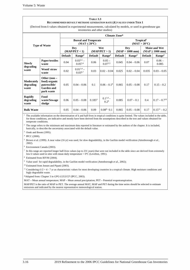
TABLE 3.3 RECOMMENDED DEFAULT METHANE GENERATION RATE (k ) VALUES UNDER TIER 1

(Derived from k values obtained in experimental measurements, calculated by models, or used in greenhouse gas inventories and other studies)

Type of Waste

Climate Zone*

Boreal and Temperate (MAT ≤ 20°C)

Tropical1

(MAT > 20°C) Dry

(MAP/PET < 1) Wet

(MAP/PET > 1) Dry

(MAP < 1000 mm) Moist and Wet

(MAP ≥ 1000 mm) Default Range2 Default Range2 Default Range2 Default Range2

Slowly degrading waste

Paper/textiles waste 0.04 0.033,5 –

0.053,4 0.06 0.05 – 0.073,5 0.045 0.04 – 0.06 0.07 0.06 –

0.085

Wood/ straw waste 0.02 0.013,4 –

0.036,7 0.03 0.02 – 0.04 0.025 0.02 – 0.04 0.035 0.03 – 0.05

Moderately degrading waste

Other (non – food) organic putrescible/ Garden and park waste

0.05 0.04 – 0.06 0.1 0.06 – 0.18 0.065 0.05 – 0.08 0.17 0.15 – 0.2

Rapidly degrading waste

Food waste/Sewage sludge

0.06 0.05 – 0.08 0.1854 0.13,4 – 0.29 0.085 0.07 – 0.1 0.4 0.17 – 0.710

Bulk Waste 0.05 0.04 – 0.06 0.09 0.088 – 0.1 0.065 0.05 – 0.08 0.17 0.1511 – 0.2

1 The available information on the determination of k and half-lives in tropical conditions is quite limited. The values included in the table, for those conditions, are indicative and mostly have been derived from the assumptions described in the text and values obtained for temperate conditions.

2 The range refers to the minimum and maximum data reported in literature or estimated by the authors of the chapter. It is included, basically, to describe the uncertainty associated with the default value.

3 Oonk and Boom (1995). 4 IPCC (2000). 5 Brown et al. (1999). A near value (16 yr) was used, for slow degradability, in the GasSim model verification (Attenborough et al.,

2002). 6 Environment Canada (2003). 7 In this range are reported longer half-lives values (up to 231 years) that were not included in the table since are derived from extremely

low k values used in sites with mean daily temperature < 0ºC (Levelton, 1991). 8 Estimated from RIVM (2004). 9 Value used for rapid degradability, in the GasSim model verification (Attenborough et al., 2002); 10 Estimated from Jensen and Pipatti (2003). 11 Considering t1/2 = 4 - 7 yr as characteristic values for most developing countries in a tropical climate. High moisture conditions and

higly degradable waste. *Adapted from: Chapter 3 in GPG-LULUCF (IPCC, 2003). MAT – Mean annual temperature; MAP – Mean annual precipitation; PET – Potential evapotranspiration. MAP/PET is the ratio of MAP to PET. The average annual MAT, MAP and PET during the time series should be selected to estimate emissions and indicated by the nearest representative meteorological station.



TABLE 3.4 RECOMMENDED DEFAULT HALF-LIFE (t1/2) VALUES (YR) UNDER TIER 1

(Derived from k values obtained in experimental measurements, calculated by models, or used in greenhouse gas inventories and other studies)

Type of Waste

Climate Zone*

Boreal and Temperate (MAT ≤ 20°C)

Tropical1

(MAT > 20°C) Dry

(MAP/PET < 1) Wet

(MAP/PET > 1) Dry

(MAP < 1000 mm) Moist and Wet

(MAP ≥ 1000 mm) Default Range2 Default Range2 Default Range2 Default Range2

Slowly degrading waste

Paper/textiles waste 17 143,5 –

233,4 12 10 – 143,5 15 12 – 17 10 8 – 12

Wood/ straw waste 35 233,4 –

696,7 23 17 – 35 28 17 – 35 20 14 – 23

Moderately degrading waste

Other (non – food) organic putrescible/ Garden and park waste

14 12 – 17 7 6 – 98 11 9 – 14 4 3 – 5

Rapidly degrading waste

Food waste/Sewage sludge

12 9 – 14 44 33,4 – 69 8 6 – 10 2 110 – 4

Bulk Waste 14 12 – 17 7 6 – 98 11 9 – 14 4 3 – 511

1 The available information on the determination of k and half-lives in tropical conditions is quite limited. The values included in the table, for those conditions, are indicative and mostly have been derived from the assumptions described in the text and values obtained for temperate conditions.

2 The range refers to the minimum and maximum data reported in literature or estimated by the authors of the chapter. It is included, basically, to describe the uncertainty associated with the default value.

3 Oonk and Boom (1995). 4 IPCC (2000). 5 Brown et al. (1999). A near value (16 yr) was used, for slow degradability, in the GasSim model verification (Attenborough et al.,

2002). 6 Environment Canada (2003). 7 In this range are reported longer half-lives values (up to 231 years) that were not included in the table since are derived from extremely

low k values used in sites with mean daily temperature < 0ºC (Levelton,1991). 8 Estimated from RIVM (2004). 9 Value used for rapid degradability, in the GasSim model verification (Attenborough et al., 2002). 10 Estimated from Jensen and Pipatti (2003). 11 Considering t1/2 = 4 - 7 yr as characteristic values for most developing countries in a tropical climate. High moisture conditions and

higly degradable waste. *Adapted from: Chapter 3 –GPG-LULUCF (IPCC, 2003). MAT – Mean annual temperature; MAP – Mean annual precipitation; PET – Potential evapotranspiration. MAP/PET is the ratio of MAP to PET. The average annual MAT, MAP and PET during the time series should be selected to estimate emissions and indicated by the nearest representative meteorological station.

METHANE RECOVERY (R) CH4 generated at SWDS can be recovered and combusted in a flare or energy device. The amount of CH4 which is recovered is expressed as R in Equation 3.1. If the recovered gas is used for energy, then the resulting greenhouse gas emissions should be reported under the Energy Sector. Emissions from flaring are however not significant, as the CO2 emissions are of biogenic origin and the CH4 and N2O emissions are very small, so good practice in the waste sector does not require their estimation. However, if it is wished to do so these emissions should be reported under the waste sector. A discussion of emissions from flares and more detailed information are given in Volume 2, Energy, Chapter 4.2. Emissions from flaring are not treated at Tier 1.

The default value for CH4 recovery is zero. CH4 recovery should be reported only when references documenting the amount of CH4 recovery are available. Reporting based on metering of all gas recovered for energy and flaring, or reporting of gas recovery based on the monitoring of produced amount of electricity from the gas (considering the availability of load factors, heating value and corresponding heat rate, and other factors

Volume 5: Waste


impacting the amount of gas used to produce the monitored amount of electricity) is consistent with good practice.

Estimating the amount of CH4 recovered using more indirect methods should be done with great care, using substantiated assumptions. Indirect methods might be based on the number of SWDS in a country with CH4 collection or the total capacity of utilisation equipment or flaring capacity sold.

When CH4 recovery is estimated on the basis of the number of SWDS with landfill gas recovery a default estimate of recovery efficiency would be 20 percent. This is suggested due to the many uncertainties in using this methodology. There have been some measurements of efficiencies at gas recovery projects, and reported efficiencies have been between 10 and 85 percent Oonk and Boom (1995) measured efficiencies at closed, unlined SWDS to be in between 10 and 80 percent, the average over 11 SWDS being 37 percent. More recently Scharff et al. (2003) measured efficiencies at four SWDS to be 9 percent, 50 percent, 55 percent and 33 percent. Spokas et al. (2006) and Diot et al. (2001) recently measured efficiencies above 90 percent. In general, high recovery efficiencies can be related to closed SWDS, with reduced gas fluxes, well-designed and operated recovery and thicker and less permeable covers. Low efficiencies can be related to SWDS with large parts still being in exploitation and with e.g., temporary sandy covers.

Country-specific values may be used but significant research would need to be done to understand the impact on recovery of following parameters: cover type, percentage of SWDS covered by recovery project, presence of a liner, open or closed status, and other factors.

When the amount of CH4 recovered is based on the total capacity of utilisation equipment or flares sold, an effort should be made in order to identify what part of this equipment is still operational. A conservative estimate of amount of CH4 generated could be based on an inventory of the minimum capacities of the operational utilisation equipment and flares. Another conservative approach is to estimate total recovery as 35 percent of the installed capacities. Based on Dutch and US studies (Oonk, 1993; Scheehle, 2006), recovered amounts varied from 35 to 70 percent of capacity rates. The reasons for the range included (i) running hours from 95 percent down to 80 percent, due to maintenance or technical problems; (ii) overestimated gas production and as result oversized equipment; (iii) back-up flares being largely inactive. The higher rates took these considerations already into account when estimating capacity. If a country uses this method for flaring, care must be taken to ensure that the flare is not a back-up flare for a gas-to-energy project. Flares should be matched to SWDS wherever possible to ensure that double counting does not occur.

In all cases, the recovered amounts should be reported as CH4, not as landfill gas, as landfill gas contains only a fraction of CH4. The basis for the reporting should be clearly documented. When reporting is based on the number of SWDS with landfill gas recovery or the total capacity of utilisation equipment, it is essential that all assumptions used in the estimation of the recovery are clearly described and justified with country-specific data and references.

DELAY TIME In most solid waste disposal sites, waste is deposited continuously throughout the year, usually on a daily basis. However, there is evidence that production of CH4 does not begin immediately after deposition of the waste.

At first, decomposition is aerobic, which may last for some weeks, until all readily available oxygen has been used up. This is followed by the acidification stage, with production of hydrogen. The acidification stage is often said to last for several months. After which there is a transition period from acidic to neutral conditions, when CH4 production starts.

The period between deposition of the waste and full production of CH4 is chemically complex and involves successive microbial reactions. Time estimates for the delay time are uncertain, and will probably vary with waste composition and climatic conditions. Estimates of up to one year have been given in the literature (Gregory et al., 2003; Bergman, 1995; Kämpfer and Weissenfels, 2001; Barlaz, 2004). The IPCC provides a default value of six months for the time delay (IPCC, 1997). This is equivalent to a reaction start time of 1st of January in the year after deposition, when the average residence time of waste in the SWDS has been six months. However, the uncertainty of this assumption is at least 2 months.

The IPCC Waste Model allows the user to change the default delay of six months to a different value. It is good practice to choose a delay time of between zero and six months. Values outside this range should be supported by evidence.



3.3 USE OF MEASUREMENT IN THE ESTIMATION OF CH4 EMISSIONS FROM SWDS

No refinement.

3.4 CARBON STORED IN SWDS No refinement.

3.5 COMPLETENESS No refinement.

3.6 DEVELOPING A CONSISTENT TIME SERIES No refinement.

3.7 UNCERTAINTY ASSESSMENT No refinement.

3.7.1 Uncertainty attributable to the method No refinement.

3.7.2 Uncertainty attributable to data Please see Section 3.7.2.2

3.7.2.1 UNCERTAINTIES ASSOCIATED WITH ACTIVITY DATA No refinement.

3.7.2.2 UNCERTAINTIES ASSOCIATED WITH PARAMETERS

Methane correction factor (MCF), Fraction of degradable organic carbon (DOC) in waste and Fraction of degradable organic carbon which decomposes (DOCf) This section provides updates on uncertainty of default DOCf value as shown in Table 3.5 (Updated). The estimates are based on DOCf derived from information reported in the literatures and expert judgement. Reported biodegradability of waste components were varied in a wide range depending on the composition of materials in bulk wastes as well as environmental factors in which the wastes are undergone biodegradation. It is recognized that laboratory experiments where some of reported DOCf values are derived from would be quite different from the real condition of SWDS but there was also some good agreement between the reported biodegradable fractions of waste components derived from laboratory experiments and observed data from field investigations. In the 2006 IPCC Guidelines, the uncertainty range of proposed default DOCf value of bulk wastes is ±20 percent which is in agreement with recent updated information on DOC percentages of ±18 percent found in SWDS (De la Cruz et al. 2013). Moreover, the proposed default DOCf values for different waste component are derived based on the information reported in the literatures.

Volume 5: Waste


TABLE 3.5 (UPDATED) ESTIMATES OF UNCERTAINTIES ASSOCIATED WITH THE DEFAULT ACTIVITY DATA AND PARAMETERS

IN THE FOD METHOD FOR CH4 EMISSIONS FROM SWDS

Activity data and emission factors Uncertainty Range

Total Municipal Solid Waste (MSWT)

Country-specific: 30% is a typical value for countries which collect waste generation data on regular basis. ±10% for countries with high quality data (e.g., weighing at all SWDS and other treatment facilities). For countries with poor quality data: more than a factor of two.

Fraction of MSWT sent to SWDS (MSWF)

±10% for countries with high quality data (e.g., weighing at all SWDS). ±30% for countries collecting data on disposal at SWDS. For countries with poor quality data: more than a factor of two.

Total uncertainty of Waste composition

±10% for countries with high quality data (e.g., regular sampling at representative SWDS). ±30% for countries with country-specific data based on studies including periodic sampling. For countries with poor quality data: more than a factor of two.

Degradable Organic Carbon (DOC)3

For IPCC default values : ±20% For country-specific values: Based on representative sampling and analyses: ±10%

Fraction of Degradable Organic Carbon Decomposed (DOCf) = 0.1 = 0.5 = 0.7

For IPCC default value (0.5): ± 20% For IPCC default value for each waste type ±90% ±70% ±30% For country-specific value ± 10% for countries based on the experimental data over longer time periods.

Methane Correction Factor (MCF) = 1.0 = 0.8 = 0.7 = 0.5 = 0.4 = 0.41 = 0.6

For IPCC default value： –10%, +0% ±20% ±30% ±20% ±30% ±60% –50%, +60%

Fraction of CH4 in generated Landfill Gas (F) = 0.5

For IPCC default value: ±5%

Methane Recovery (R) The uncertainty range will depend on how the amounts of CH4 recovered and flared or utilised are estimated: ± 10% if metering is in place. ± 50% if metering is not in place.

Oxidation Factor (OX) Include OX in the uncertainty analysis if a value other than zero has been used for OX itself. In this case the justification for a non-zero value should include consideration of uncertainties.

half-life ( t1/2 ) Ranges for the IPCC default values are provided in Table 3.4. Country-specific values should include consideration of uncertainties.

Source: Expert judgement by Lead Authors of the Chapter. 1MCF for Managed well – active aeration

3.8 QA/QC, Reporting and Documentation No refinement.

3 The uncertainty range given applies to the DOC content in bulk waste. The ranges for DOC for different waste components

in MSW given in Table 2.4 can be used to estimate the uncertainties for these components.



References References newly cited in the 2019 Refinement

Bayard, R., Benbelkacem, H., Gourdon, R. & Buffière, P. (2018) Characterization of selected municipal solid waste components to estimate their biodegradability. Journal of Environmental Management 216: 4-12.

De la Cruz, F.B., Chanton, J.P. & Barlaz, M.A. (2013) Measurement of carbon storage in landfills from the biogenic carbon content of excavated waste samples. Waste Management 33: 2001-2005.

Eleazer, W.E., Odel III, W.S., Wang, Y.S. & Barlaz, M.A. (1997) Biodegradability of municipal solid waste components in laboratory-scale landfills. Environmental Science and Technology 31: 911-917.

Hrad, M., Gamperling, O. & Huber-Humer, M. (2013) Comparison between lab- and full-scale applications of in situ aeration of an old landfill and assessment of long-term emission development after completion. Waste Management 33: 2061-2073.

Ishigaki,T., Nakanishi A., Tateda, M., Ike, M. & Fujita M. (2003) Application of Bioventing to Waste Landfill for Improving Waste Settlement and Leachate Quality - A Lab Scale Model Study. Journal of Solid Waste Technology and Management 29(4): 230-238.

Jeong S. (2016) Verification of Methodologies and Estimation of IPCC Model Parameters for Solid Waste Landfills, Ph.D. Dissertation, Seoul National University, 141 pp.

Jiang, J., Yang, G., Deng, Z., Huang, Y., Huang, Z., Feng X., Zhou, S. & Zhang, C. (2007) Pilot-scale experiment on anaerobic bioreactor landfills in China. Waste Management 27: 893-901.

Karanjekar, R. V., Bhatt, A., Altouqui S., Jangikhatoonabad, N., Durai, V., Sattler, M., Hossain, M.D.S. & Chen V. (2015) Estimating methane emissions from landfills based on rainfall, ambient temperature, and waste composition: The CLEEN model. Waste Management 46: 389-398.

Laboratory of Solid Waste Disposal Engineering (2016) Study on semi-aerobic landfill site measuring gas flow rate and temperature, Hokkaido University, Japan

Raga, R. & Cossu, R. (2014) Landfill aeration in the framework of a reclamation project in Northern Italy. Waste Management 34: 683-691.

Ritzkowski, M., Heyer, K.U. & Stegmann, R. (2006) Fundamental processes and implications during in situ aeration of old landfills. Waste Management 26: 356-372.

Ritzkowski, M. & Stegmann, R. (2012) Landfill aeration worldwide: Concepts, indications and findings. Waste Management 32: 1411-1419.

Ritzkowski, M. & Stegmann, R. (2013) Landfill aeration within the scope of post-closure care and its completion, Waste Management 33: 2074-2082.

Ritzkowski, M., Walker, B., Kuchta, K., Raga, R. & Stegmann, R. (2016) Aeration of the teuftal landfill: Field scale concept and lab scale simulation, Waste Management 55: 99-107.

Sutthasil, N., Chiemchaisri, C., Chiemchaisri, W., Wangyao, K., Towprayoon, S., Endo, K. & Yamada, M. (2014) Comparison of Solid Waste Stabilization and Methane Emission from Anaerobic and Semi-Aerobic Landfills Operated in Tropical Condition. Environmental Engineering Research , 19(3): 261-268.

Tsubaki, M., Ueno, S. & Tsuji, Y. (2009) The CDM Metrodology for Reduction of Greenhouse Gas Emission from Landfull Sites by Semi-aerobic Landfill System. In: Sardinia 2009, Twelfth International Waste Management and Landfill Symposium, Italy.

UNFCCC CDM Executive Board (2009) Approved baseline and monitoring methodology AM0083 “Avoidance of landfill gas emissions by in-situ aeration of landfill” AM0083 / Version 01.0.1

Wang, X. & Barlaz, M.A. (2016) Decomposition and carbon storage of hardwood and softwood branches in laboratory-scale landfills. Science of the Total Environment 557-558: 355-362.

Wang, X., De la Cruz, F.B., Ximenes, F. & Barlaz, M.A. . (2015) Decomposition and carbon storage of selected paper products in laboratory-scale landfills. Science of the Total Environment 532: 70-79.

Wang, X., Padgett, J.M., De le Cruz, F.B. & Barlaz M.A. (2011) Wood biodegradation in laboratory-scale landfills. Environmental Science and Technology 45: 6864-6871

Ximenes, F., Björdal, C., Cowie, A. & Barlaz, M.A. (2015) The decay of wood in landfills in contrasting climates in Australia. Waste Management 41: 101-110.

Volume 5: Waste


Ximenes, F.A., Cowie, A.L. & Barlaz, M.A. (2018) The decay of engineered wood products and paper excavated from landfills in Australia. Waste Management 74: 312-322.

Yamada M., Ishigaki T., Endo K., Ishimori H., Wangyao K., Sutthasil N. & Chiemchaisri C. (2013) Numerical Analysis of Efficiency of Semiarobic Management of Landfill, Proceedings of the 14th International Waste Management and Landfill Symposium 14: 389.

Zhan, L. T., Xu, H., Chen, Y.M., Lan, J.W., Lin W.A., Xu, X.B. & He P.J. (2017) Biochemical, hydrological and mechanical behaviors of high food waste content MSW landfill: Liquid-gas interactions observed from a large-scale experiment. Waste Management 68: 307-318.

References copied from the 2006 IPCC Guidelines

Barrow, Gordon M. (1996). Physical Chemistry, Mc Graw Hill, NewYork, 6th ed.

IPCC (2000). Good Practice Guidance and Uncertianty Management in National Greenhouse Gas Inventories. Penman, J., Kruger D., Galbally, I., Hiraishi, T., Nyenzi, B., Enmanuel, S., Buendia, L., Hoppaus, R., Martinsen, T., Meijer, J., Miwa, K. and Tanabe, K. (Eds). Intergovernmental Panel on Climate Change (IPCC), IPCC/OECD/IEA/IGES, Hayama, Japan.

IPCC (1997). Revised 1996 IPCC Guidelines for National Greenhouse Inventories. Houghton, J.T., Meira Filho, L.G., Lim, B., Tréanton, K., Mamaty, I., Bonduki, Y., Griggs, D.J. and Callander, B.A. (Eds). Intergovernmental Panel on Climate Change (IPCC), IPCC/OECD/IEA, Paris, France.

Pingoud, K. and Wagner, F. (2006). Methane emissions from landfills and decay of harvested wood products: the first order decay revisited. IIASA Interim Report IR-06-004.



Appendix 3A.1 Information on Nitrous Oxide Emission from Solid Waste Disposal Site

Significant generation of N2O from SWDS was indicated by the IPCC Fourth Assessment Report (2007). However, the 2006 IPCC Guidelines do not present a methodlogy or parameters by which N2O emissions can be estimated.

The approved CDM methodology, AM0083 (UNFCCC CDM Executive Board 2009), is applicable to project activities where landfilled waste is treated aerobically on-site by means of air venting (overdrawing) or low pressure aeration with the objective of avoiding anaerobic degradation processes and achieving aerobic degradation. The AM0083 provides two alternative methodologies for estimating N2O emissions. One is estimation based on measured N2O on the site, and the other is using emission factor. The aerobic pathway of N2O generation in SWDS is well known (Borjesson & Svensson 1997; He et al. 2011; Harborth et al. 2013), and the emission factor given in AM0083 is based on waste composting (0.2-1.6 g N2O/kg waste treated on a dry weight base or 0.06-0.6 g N2O/kg waste treated on a wet weight base), which is regarded as an analogue process to low pressure aeration. While the properties of waste in SWDS or aeration rate adopted in the active aeration are far from the condition of composting, it is recommended to obtain the local monitoring data to be used for estimation of N2O emission from SWDS.

Not only active aeration of managed landfills but cover soils and working faces in all SWDS are potential emission sources of N2O because these zones are allowed to penetrate atmospheric oxygen diffusively. Emission of N2O has not been reported in semi-aerobically managed landfills while not so many information is available. If the specific project on active aeration of SWDS in each country is adopted for emission estimation, and if it also reported N2O emission as well in accordance with AM0083, that can also be taken into consideration for inventory reports.

The anaerobic generation of N2O is also common and has been observed in SWDS (Rinne et al. 2005; Matthew et al. 2005; Ishigaki et al. 2016). Anaerobic pathway of N2O generation is combined with denitrification process and is correlated to anaerobic decay of DOC. There are two uncertainties on the degree of conversion of nitrogen compounds to N2O and the degree of carbon consumption by nitrogen conversion for the emission estimation. Apparent correlation of N2O and CH4 emissions was obtained about 20 percent by equivalent to CO2 in anaerobically managed landfills (Ishigaki et al. 2016), whereas it requires to validate for country specific condition in order to obtain reliable emission estimate.

REFERENCES Börjesson, G. & Svensson B.H. (1997) Nitrous oxide emissions from landfill cover soils in Sweden, Tellus B:

Chemical and Physical Meteorology, 49(4): 357-363.

Harborth, P., Fuss, R, Münnich, K, Flessa, H. & Fricke, K. (2013) Spatial variability of nitrous oxide and methane emissions from an MBT landfill in operation: strong N2O hotspots at the working face. Waste Manag. 33(10): 2099-2107.

He, P., Yang, N., Gu, H., Zhang, H. & Shao, L. (2011) N2O and NH3 emissions from a bioreactor landfill operated under limited aerobic degradation conditions. Journal of Environmental Sciences, 23(6): 1011-1019.

Ishigaki, T., Nakagawa, M., Nagamori, M. & Yamada, M. (2016) Anaerobic generation and emission of nitrous oxide in waste landfills. Environ Earth Sci. 75: 750.

IPCC, 2007: Climate Change 2007: Mitigation. Contribution of Working Group III to the Fourth Assessment Report of the Intergovernmental Panel on Climate Change [B. Metz, O.R. Davidson, P.R. Bosch, R. Dave, L.A. Meyer (eds)], Cambridge University Press, Cambridge, United Kingdom and New York, NY, USA., 385-618pp.

McBain, M.C., Warland, J.S., McBride, R.A. & Wagner-Riddle, C. (2005) Micrometeorological measurements of N2O and CH4 emissions from a municipal solid waste landfill. Waste Manage Res. 23: 409-419.

Rinne, J., Pihlatie, M., Lohila, A., Thum, T., Aurela, M., Tuovinen, J.P., Laurila, T. & Vesala, T. ( 2005) Nitrous Oxide Emissions from a Municipal Landfil . Environ Sci Technol. 39(20): 7790-7793.

UNFCCC CDM Executive Board (2009) Approved baseline and monitoring methodology AM0083 “Avoidance of landfill gas emissions by in-situ aeration of landfill” AM0083 / Version 01.0.1

Volume 5: Waste


Appendix 3A.2 Information on Estimation of CH4 Emission from Solid Waste Disposal Site Managed by Active Aeration Using Locally Available Measured Data

Estimation of MCF for Active Aeration Using Measured Data The practice of implementation of active aeration of SWDS is very limited. Therefore, improvement of the default values of MCF for active aeration shown in Table 3.1 (Updated) is necessary. Estimation of the FOD parameters by locally available direct measured data on landfill gas emission in SWDS is encouraged by the 2006 IPCC Guidelines (Chapter 3.3, Volume 5). Direct measured of gas emission at SWDS managed by active aeration, which are normally collected as operational data, can be also applied for estimating MCF. Stable operational conditions of aeration of SWDS is still under development, therefore monitoring data tends to fluctuate even in the same country. Assessment of uncertainty of local monitoring data is indispensable before estimating the emission in this category.

MCF for SWDS managed by active aeration is determined by measured data of CH4 and CO2 in landfill gas.

EQUATION 3AP.1 (NEW) MCF FOR MANAGED SWDS (ACTIVE AERATION)

( ) ( )' ' 112

P P Q QMCF

P− + − = −

Where:

P = fraction of CH4 measured in landfill gas at cell managed anaerobically or before active aeration (fraction)

P’ = fraction of CH4 measured in landfill gas during active aeration (fraction), P’ ≤ P

Q = fraction of CO2 measured in landfill gas at cell managed anaerobically or before active aeration (fraction)

Q’ = fraction of CO2 measured in landfill gas during active aeration (fraction), Q’ ≥ Q

This method is suitable if fraction of CH4 and CO2 are measured at systems of forced extraction or suction of landfill gas. In other case variance of measured data is high and careful assessment of validity of data is essential. Uncertainty and consistency of MCF and estimated emission is also evaluated.

Default value for fraction of CH4 in generated landfill gas (0.5) is given in the 2006 IPCC Guidelines (Chapter 3.2.3, Volume 5). As stated there, fraction of CH4 in generated landfill gas must not be confused with measured CH4 in landfill gas emitted, because CO2 generated is absorbed in seepage water. Even if the fractions of CH4 and CO2 measured in landfill gas at a cell managed anaerobically or before active aeration (P and Q) are not available, using default value for fraction of CH4 in generated landfill gas (F) is not recommended, and adjustment of CO2 absorption in seepage water is required. Consideration of CH4 oxidation is also necessary when it is enhanced by active aeration.

Estimation of Emissions Using Measurements of Flow Rates and CH4 Concentrations While consistent measured data of fractions of CH4 and CO2 in landfill gas is not available or its validity is poor, direct estimation of CH4 emission by using measured data in individual SWDS is encouraged.

To monitor actual CH4 emissions from the aerated landfill, both surface and vented emissions from the surface have to be measured. As shown in the 2006 IPCC Guidelines (Chapter 3.3, Volume 5), measurement of gases in collection system and fugitive emission through the surface are covered.

CH4 emission from gas collection system is obtained as the product of content of CH4 (Gg/m3) and flow rate of the landfill gas from the pipe (m3/yr). Flow rate of landfill gas is estimated by multiplying the velocity of gas in certain depth by the area of the pipe. When forced extraction is implemented, CH4 emission from gas collection system dominate and reliable and representative data are obtained. Even though, it is necessary to take into consideration the variance of emissions in each well for accurate estimation. At least quarterly measurements should be done within each venting well in order to account for the seasonal variation of emissions.

CH4 emission from surface of SWDS is obtained by several methods shown in Box 3.2 in the 2006 IPCC Guidelines. Representativeness and coverage of surface emission should be carefully considered. Since results



obtained by flux chamber method fluctuate to a great extent from one zone to other within the same SWDS, a number of measurement points is required to express the surface distribution of emissions. Geostatistical analysis methods should be applied in order to obtain representative data of emissions from fluctuated fluxes in different zones of the SWDS. The SWDS can be subdivided into different zones with distinctive characteristics with regard to expected surface emissions. A flux density of the landfill gas (mg/m2•s) can be calculated for each measurement. Then, average surface emissions rate can be calculated for each zone by multiplying the average flux density with the corresponding area of the zone. Due to the high uncertainty of surface measurements, a conservativeness factor should be used to account for such uncertainties. For example, a conservativeness factor of 1.37 is multiplied by CH4 emission from surface emissions is proposed by UNFCCC CDM Executive Board (2009).

REFERENCES UNFCCC CDM Executive Board (2009) Approved baseline and monitoring methodology AM0083 “Avoidance

of landfill gas emissions by in-situ aeration of landfill”, AM0083 / Version 01.0.1

CHAPTER 3 SOLID WASTE DISPOSAL...2019 Refinement to the 2006 IPCC Guidelines for National Greenhouse...

Documents

Transcript of CHAPTER 3 SOLID WASTE DISPOSAL...2019 Refinement to the 2006 IPCC Guidelines for National Greenhouse...