44

CHAPTER 3

SIMULATION OF FOUR QUADRANT OPERATION IN

THREE PHASE BLDC MOTOR USING

MATLAB/SIMULINK

3.1 INTRODUCTION

Simulink platform is effective in the simulation and analysis of

dynamic systems. With Simulink, experimental models can be easily built

from the scratch and existing models can be modified to the user’s needs.

Linear and nonlinear systems, modelled in continuous time, sampled time, or

a hybrid of the two are supported by Simulink. Systems can also be

multirate— having different parts that are sampled or updated at different

rates. This chapter presents a Simulink model in MATLAB R2011a to

simulate the four quadrant operation of three-phase BLDC motor. This

simulation includes the closed loop control of the motor.

3.2 BLOCK DIAGRAM REPRESENTATION OF THE DRIVE

SYSTEM

The three-phase BLDC motor with built in Hall sensors is chosen

for this research work. The Hall sensors are required to detect the rotor

position and they have to be fed back into the controller. The reference speed

is fed as an input to the controller. Eventually, the controller generates the

PWM pulses required to commutate the switches according to its input. The

implementation of the proposed drive system is presented in Figure 3.1.

45

Figure 3.1 Complete Drive System

The three-phase inverter is supplied from a DC source. The inverter

circuit is coupled to the motor using normally closed contacts. During

motoring operation, the PWM pulses provide the appropriate switching

sequence to the inverter.

The switching (relay) circuit is coupled to the BLDC motor.

Whenever the motor is operating in the regenerative mode, the normally open

contacts of the switching circuit get closed. Thereby the generated voltage

gets rectified and the charge gets stored in the chargeable battery.

3.3 SIMULINK MODEL OF BLDC DRIVE

The proposed Simulink model of BLDC drive is shown in Figure

3.2. The controller gets the position of the rotor from the Hall signals and the

actual speed of the motor is also fed as an input. The controller generates the

gate signals as its output, which will be fed to the inverter circuit.

46

Figure 3.2 Simulink Model of Drive System

The different loads to be applied at various instants are also

modelled. The Hall signals, PWM pulses, stator EMFs and stator currents of

the three phases, the actual rotor speed, and the achieved speed control are

captured using the scope. The simulation time is 3 s and the power GUI is

continuous. The battery characteristics, namely the battery voltage, the

charging current and the charging status are also obtained in the scope.

3.3.1 BLDC Motor

Three-phase Permanent Magnet Synchronous Motor (PMSM), with

trapezoidal back EMF is configured as a model of BLDC motor in the

simulation. The stator windings are connected in star to an internal neutral

point. The rotor is non-salient pole type with trapezoidal flux pattern in the air

gap. The motor parameters are presented in Figure 3.3. The Hall signals and

the actual rotor speed are obtained as output from the motor.

47

Figure 3.3 Motor Parameters

3.3.2 Controller

The controller subsystem comprising of decoder and gate signals

generator is shown in Figure 3.4. The decoder receives Hall signals as its

input and the excitation voltages of the three-phases are generated as output by

the decoder. While the excitation voltages and the actual speed of the rotor are the

input to the gate signals generator, the PWM pulses (gate signals) are its output.

Figure 3.4 Controller – Subsystem

48

The decoder subsystem is shown in Figure 3.5.

Figure 3.5 Decoder–Subsystem

The excitation sequence of the phases a, b and c of the three-phase

BLDC motor for clock wise and counter clockwise direction of rotation of

motor are given in Table 3.1 and Table 3.2 respectively. Ha, Hb and Hc

represent the Hall sensor signals and EMFA, EMFB and EMFC represent the

excitation of phases A, B and C respectively.

Table 3.1 Sequence of excitation of phases – clockwise

Ha Hb Hc EMFA EMFB EMFC

0 0 0 0 0 0

0 0 1 0 -1 +1

0 1 0 -1 +1 0

0 1 1 -1 0 +1

1 0 0 +1 0 -1

1 0 1 +1 -1 0

1 1 0 0 +1 -1

1 1 1 0 0 0

49

Table 3.2 Sequence of excitation of phases – counter clockwise

Ha Hb Hc EMFA EMFB EMFC

0 0 0 0 0 0

0 0 1 0 +1 -1

0 1 0 +1 -1 0

0 1 1 +1 0 -1

1 0 0 -1 0 +1

1 0 1 -1 +1 0

1 1 0 0 -1 +1

1 1 1 0 0 0

3.3.3 Gate Signal Generation

The gate signal generator subsystem is displayed in the Figure 3.6.

The gate signals are generated from the decoder excitation voltages, after the

logical operations.

Figure 3.6 Gate Signal Generator–Subsystem

50

The commutation sequence implemented by the gate signal

generator is presented in Table 3.3 and Table 3.4 for clockwise and counter

clockwise direction respectively.

Table 3.3 Commutation Sequence – Clockwise

Ha Hb Hc EMFA EMFB EMFC S1 S2 S3 S4 S5 S6

0 0 0 0 0 0 0 0 0 0 0 0

0 0 1 0 -1 +1 0 0 0 1 1 0

0 1 0 -1 +1 0 0 1 1 0 0 0

0 1 1 -1 0 +1 0 1 0 0 1 0

1 0 0 +1 0 -1 1 0 0 0 0 1

1 0 1 +1 -1 0 1 0 0 1 0 0

1 1 0 0 +1 -1 0 0 1 0 0 1

1 1 1 0 0 0 0 0 0 0 0 0

Table 3.4 Commutation Sequence – Counter Clockwise

Ha Hb Hc EMFA EMFB EMFC S1 S2 S3 S4 S5 S6

0 0 0 0 0 0 0 0 0 0 0 0

0 0 1 0 -1 +1 0 0 1 0 0 1

0 1 0 -1 +1 0 1 0 0 1 0 0

0 1 1 -1 0 +1 1 0 0 0 0 1

1 0 0 +1 0 -1 0 1 0 0 1 0

1 0 1 +1 -1 0 0 1 1 0 0 0

1 1 0 0 +1 -1 0 0 0 1 1 0

1 1 1 0 0 0 0 0 0 0 0 0

The reference speed for the rotor is compared with the actual rotor

speed and error signal is passed on to the PI controller. The Kp and Ki values

51

are obtained as 1.0 by trial and error method. The PI controller’s output is

applied to the PWM generator block. This block generates pulses for carrier

based PWM, self-commutated IGBTs. The carrier frequency is assumed as

1080 Hz with a modulation index of 0.4.

PI controller is chosen due to its ease in design and simple

structure. The proportional (P) term of the controller is formed by multiplying

the error signal by a P gain, causing the PI controller to produce a control

response which is a function of the error magnitude. As the error signal

becomes larger, the P term of the controller becomes larger to provide more

correction. The effect of the P term tends to reduce the overall error as time

goes by. However the P term has less effect as the error approaches zero. In

most systems, the error of the controlled parameter gets very close to zero but

does not converge. The result is a small remaining steady state error.

The integral (I) term of the controller is used to eliminate small

steady state errors. The term I calculates a continuous running total of the

error signal. Therefore a small steady state error accumulates in to a large

error value over time. This accumulated error signal is multiplied by a gain

factor I and becomes the output term I of the PI controller. In the proposed

system, the PI controller is conventional and simple to achieve the desired

steady state response of the speed.

3.3.4 Regenerative Mode

The relay block subsystem for the regeneration process is shown in

Figure 3.7. Three switches are provided, which are normally open contacts of

relay coil. The normally open contacts are closed when the actual speed goes

below zero rpm. This happens when the brake is applied or when there is

reversal in direction of motor rotation. This results in the storage of the energy

in the battery. Otherwise, the brake energy will be dissipated as heat energy.

52

Figure 3.7 Relay Block – Subsystem

During the second and fourth quadrant operations, the BLDC

machine behaves like a generator and the generated voltage is used to charge

the battery. The rectifier converts the obtained AC voltage to DC of the

BLDC motor during the generation mode, to charge the battery. The

parameters of the battery are shown in Figure 3.8. The charge status is assumed

initially as 0%.

Figure 3.8 Battery Parameters

53

3.4 SIMULATION RESULTS

This section deals with the results obtained from the developed

Simulink model. The analyses of the results are presented as two case studies.

In the first case, the motor is on no-load, that is the applied load torque is

maintained at zero; the reference speed is specified and the actual speed is

observed.

In the second case, the load torque is applied at different instants

and the performance variables are observed. The load and the reference speed

are varied and the response of the machine is observed, as it operates in all the

four quadrants.

3.4.1 Speed Control at No-Load

In Table 3.5, the actual speeds obtained at different instants of time

under no-load conditions are compared with the reference speed of the rotor.

Table 3.5 Speed Control

Time (s) 0 0.5 1.0 1.5 2.0 2.5 3.0

Reference Speed (rpm) 0 200 300 400 400 300 200

Actual Speed (rpm) 0 200 300 400 400 300 200

The simulation is carried out for a time of 3 s and the continuous

power GUI mode is adopted. The Hall signals observed for the initial two

seconds are shown in Figure 3.9. The Hall signals received are lesser when

the speed is less from time 0.5 s to 1.0 s, but as the speed increases at 2 s the

Hall signals appear clustered and a frequent change in the position of the rotor

is observed.

54

Figure 3.9 Hall Signals – No load

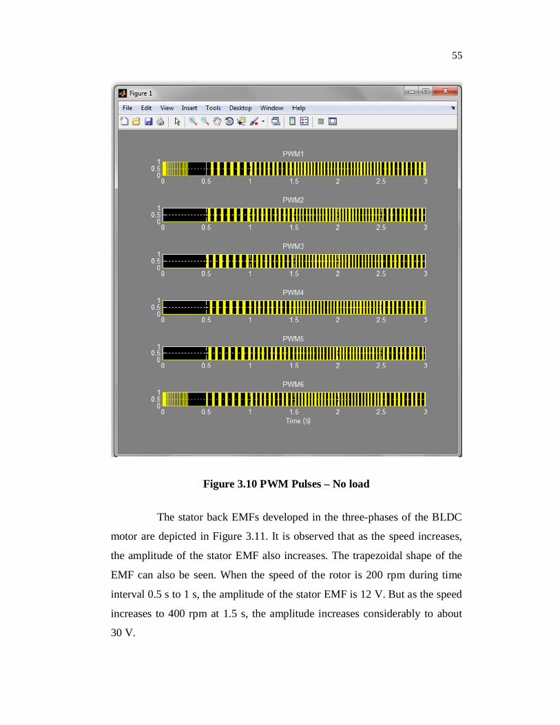
The PWM pulses applied to the inverter circuit are obtained

according to the commutation sequence are shown in Figure 3.10. All the six

pulses which are input to the six IGBTs of the inverter circuit are captured in

the scope.

(s)

55

Figure 3.10 PWM Pulses – No load

The stator back EMFs developed in the three-phases of the BLDC

motor are depicted in Figure 3.11. It is observed that as the speed increases,

the amplitude of the stator EMF also increases. The trapezoidal shape of the

EMF can also be seen. When the speed of the rotor is 200 rpm during time

interval 0.5 s to 1 s, the amplitude of the stator EMF is 12 V. But as the speed

increases to 400 rpm at 1.5 s, the amplitude increases considerably to about

30 V.

(s)

56

Figure 3.11 Stator back EMFs – No load

The stator currents of the three phases (Figure 3.12) clearly show a

spike at 0.5 s, 1s, 1.5 s and 2.5 s. These are the instants at which there is a

change in the speed of the BLDC motor.

(s)

57

Figure 3.12 Stator Currents – No load

The actual rotor speed in rpm and the electromagnetic torque in Nm

developed in the motor are shown separately in Figure 3.13. It is observed

that the developed torque is continuous.

(s)

58

Figure 3.13 Rotor Speed and Electromagnetic Torque – No load

The actual speed attains the steady state in a very short span of time

and settles down too quickly at the reference speed. The stator currents and

actual speed obtained, for no-load condition are presented in Figure 3.14.

(s)

59

Figure 3.14 Stator Currents & Actual Speed – No load

3.4.2 Four Quadrant Operation

The operation of the BLDC motor in all the four quadrants is

simulated and the results are presented in this section. In Table 3.6, the

reference speed, the applied load torque and the quadrant it belongs to, for a

time period of 3 s, are presented. The simulation time is 3 s and continuous

power GUI mode is adopted.

(s)

60

Table 3.6 Quadrant Determination

Time 0 0.5 1.0 1.75 2.0 2.5 2.75 3.0

Reference Speed (rpm) 0 200 200 200 0 -200 -200 0

Applied Load Torque (Nm) 0 0 +1 -1 -1 -1 +1 +1

Quadrant Initial I I II II III IV

For the simulation study,

From start up to 1.0 s, the torque applied is positive. That is,

the machine is operating in the first quadrant, forward

motoring.

At time 1.75 s negative torque is applied. This implies that a

sudden brake is applied. The rotor speed is drastically brought

to zero at 2.0 s; this is the second quadrant of operation,

forward braking.

At 2.5 s the motor is forced to rotate in the reverse direction,

the applied torque remains negative. Since torque and speed

are negative, the motor is operating in the third quadrant,

reverse motoring.

While at 2.75 s the load torque applied is positive, this is

reverse motoring and sudden brake is applied which drops

down the rotor speed to zero rpm, indicating that the motor is

in the fourth quadrant, reverse braking, of speed torque

characteristics.

61

The Hall signals from the Hall sensors of the BLDC machine

shows the difference in the pulse pattern during the four quadrants of

operation over the simulated time of 3 s (Figure 3.15).

Figure 3.15. Hall Signals

The PWM pulses applied to the inverter as found in Figure 3.16

shows the distribution of pulses.

(s)

62

Figure 3.16 PWM pulses

The variation in the amplitude of the stator back EMFs of all the

three phases are clearly visible in the scope results shown in Figure 3.17. The

trapezoidal shape is also seen. At the instant, when the load torque becomes

negative, the amplitude of the back EMF increases to about 58 V. When brake

is applied at time 2.75 s, the amplitude of stator back EMF reduces to zero.

(s)

63

Figure 3.17 Stator Back EMFs

Figure 3.18 shows the different patterns of the stator currents for

the four quadrants of operation. The transition from one quadrant to another is

clearly observed in this waveform. The sharp spikes at 0.5 s and 2.5 s indicate

the start of the motor and the change in direction of rotation of the motor.

(s)

64

Figure 3.18 Stator Currents

The actual rotor speed in rpm is shown in Figure 3.19. When the

applied torque is positive, the motor attains the reference speed with few

oscillations. But when negative load torque is applied, the reference speed is

not attained as it aids the motor to run. Again when the positive load torque is

applied at 2.75 s, the motor settles down to the reference speed as expected.

(s)

65

Figure 3.19 Rotor Speed and Electromagnetic Torque

The electromagnetic torque is developed during the operation of the

motor in all of its four quadrants which is also depicted in Figure 3.19. The

developed torque is also negative between 1.75 s and 2.75 s. After 2.75 s, the

electromagnetic torque builds up to become positive.

The reference speed and the actual rotor speed obtained in the same

reference scale are displayed in Figure 3.20 in order to observe the deviation

in the speed during the application of negative torque.

66

Figure 3.20 Speed Control

From Figures 3.14 and 3.20, on comparison, it is observed that

speed control is better under no-load conditions than when applying a

negative torque. When the motor is not loaded, the actual speed follows the

reference speed and attains the steady state. But during the negative torque

condition, the actual speed does not follow the reference speed, as the

negative torque aids the motor to increase its speed.

67

3.4.3 Regenerative Mode

When the machine is operating in the second and fourth quadrants,

it is said to be in the regenerative mode. During these modes of operation, the

kinetic energy will be wasted as heat energy when brake is applied. In the

proposed system, effective utilisation of this energy is attempted. Hence, the

relay block of the Simulink model closes the normally open contacts and

returns back the energy through a rectifier to be stored in a chargeable battery.

The battery voltage, the battery charging current and the charge status of the

battery which is initially zero is shown in Figure 3.21. At 1.75 s, the battery

has attained the full charge of 100%. When the negative torque is applied, the

battery voltage and current becomes zero.

Figure 3.21 Battery Characteristics

68

Energization of the battery at various operating conditions such as

different applied torques, both positive and negative and with various

directions of rotation, clockwise and counter clockwise are presented in

Table 3.7.

The table indicates that maximum energization is in the first

quadrant followed by the fourth quadrant, where the torque applied is

positive. When the torque becomes negative it results in very less or no

energization of the battery.

Table 3.7 Energization of Battery

Quadrant Applied Load Torque (Nm)

Reference Speed (rpm)

% Charge Status

I

3 100 494 100 585 100 656 100 68

II

-3 100 0.37-4 100 0.37-5 100 0.37-6 100 0.37

III

-3 -100 0.36-4 -100 0.37-5 -100 0.37-6 -100 0.37

IV

3 -100 0.44 -100 2.55 -100 126 -100 18

69

3.5 CONCLUSION

The speed control achieved through the simulation of a three-phase

BLDC motor during no-load and on-load conditions are discussed. The

possibility of energising a battery during the regenerative braking period is

reviewed. The hardware realisation of the proposed Simulink model will be

presented in the forthcoming chapter.