Chapter 3 Robot Vision 1

Chapter 3 Robot Vision

A brief Introduction Mobile robot perception is an interesting field of study and

has evolved from ad-hoc solutions to specific robot situations

to more grounded theory. Robots can be equipped with

human-like senses (vision, sound, touch) but these can be

supplemented with various others. Ultrasonic ‘ping’

rangefinders are perhaps inspired by the bat, motion detection

by the fly eye. The compass could be likened to bird-brain

sensory areas; it’s interesting to look for natural analogues of

other sensors such as GPS, wheel encoders, gyroscopes, laser

rangefinders and doppler sensors.

Sensors can be classified as exteroceptive, those

which respond to the external environment, such as vision,

and proprioceptive, those which respond the robot’s insides,

such as battery voltage, wheel position and wheel load.

Human vision is both a powerful sensory medium and is

incredibly difficult to mimic in a robotics context; remember

that over 50% of our brain is devoted to solving vision

problems. Compared with other sensors, such as laser range-

finding which responds to one (or a few) objects in a scene,

robot vision has the potential to give information about the

entire scene structure. The laser range-finder sends out a ray,

and its collision with an object occurs at a particular angle

and distance, whereas a camera has a field of view and can

report all objects within that field. Usually images are

processed before analysis; this may include edge-detection,

segmentation and object labelling, or specific transforms

which return information about straight lines, extracted by

combing edges (Hough transform).

Nature of Computing 2

Limitations First, we must accept the limitations of developing Computer

Vision solutions for the small mobile robots, often based on

Arduino technology we encounter. The first limitation is

memory size. Consider a small image of resolution 300x200

with three colour channels, i.e., 3 bytes per pixel, which

requires 180 kB of storage. The Arduino Mega2560 has 8 kB

of data memory; clearly you cannot run image processing

algorithms on this MPU, since there cannot be an image in

memory! The second limitation is processing speed; take a

300x200 grey-scale image, performing a convolution with a

3x3 kernel, at a rate of 60 fps, requires a MPU clock speed of

over 60 MHz whereas the Arduino gives us 16 MHz.

How can this be solved? Some companies offer

Arduino-compatible alternatives with huge memory and fast

processors (e.g, the Maixduino has 8 MB of data memory and

runs at 400 MHz and retails at around £25). These boards

mainly use the STMicroelectronics ‘Cortex’ MCU which is

industry standard; the Maixduino board supplements this

with a Kendryte AI processor. Compared with the Arduino,

these boards are often tricky to bring into service, and

documentation and blogs are hard to find, however we have

had recent success getting the Maixduino up and running

using PlatformIO. Then, of course, we could cross over to the

dark-side and use a Raspberry-Pi, or even the NVIDIA Jetson

technology.

Another solution is to off-load vision processing to a

dedicated board, which applies one or more image processing

algorithms, and sends the extracted features (such as

segmented object sizes) to the Arduino for analysis. A feature

can be coded in a few bytes, so memory space and transfer

and processing rates is not an issue. This is the solution we

shall encounter, our ‘Pixy2’ camera and processing board,

which runs algorithms to (i) detect coloured blobs and return

their location and size, (ii) detect lines, returning their

endpoints as (x,y) coordinates in the image, (iii) detect types

of intersections between lines. These are useful functions for

Chapter 3 Robot Vision 3

Figure 1 Pin-hole camera viewed from the top.

Rays from the red object (width W) pass through

the pinhole and create an image of size x on the

camera's CCD retina.

Figure 2 Arrangement we shall use in the lab,

where the geometrical discussion is still valid.

a Robot Vision system, as we shall see. In addition, Pixy2 lets

us extract individual pixels from the image, so we could just

about code our own algorithm, e.g., a multi-line detector. This

device is impressive, it boasts a dual-core 204 MHz NXP

LPC4330 processor with an Aptina MT9M114 1296 x 976

resolution camera.

Pin-hole Camera This is the simplest possible camera which you may have

encountered in GCSE Physics and is a good approximation

for many lens-based cameras. Look at Fig.1 showing a top

view of a camera. Rays (green) from the red object pass

through the camera iris (pin-hole) and form an image on the

charge-coupled-device (CCD) retina. Sizes and distances are

shown. The variable 𝑥 is what we observe from the camera

(and our code will report this). We need to know how to

deduce the distance L of the object from the camera. We

certainly do not know the value of d and we would like not to

have to measure the width W directly.

But let’s first remind ourselves of the geometry. Using similar

triangles, we have

𝑥

𝑑=

𝑊

𝐿

therefore

𝐿 = (𝑊𝑑

𝑥) (1)

This tells us that if we measure a small image width x then

the object is far from the camera. Now, let’s say we place an

object at a known distance 𝐿0 from the camera, and we

measure the corresponding image size 𝑥0, then substituting

into (1) we have

𝐿0 = (𝑊𝑑

𝑥0) (2)

and dividing (1) by (2) we find

Nature of Computing 4

𝐿 =1

𝑥(𝐿0𝑥0) (3)

This is useful, since the quantities in the bracket are known

(we measure them), so we can deduce any distance L from

the image width x, returned by our code. This is the process

of calibrating our camera, preparing it for use. Note the units

of the variables in (3). Both 𝐿 and 𝐿0 are measured in physical

units (e.g. mm) but the x values are measured in pixels.

A Worked Example Suppose we calibrate the camera. Assume the camera width

resolution is 320 pixels. We choose to place the object so that

its image completely fills the camera width. Let’s assume we

find this occurs at an object distance of 100 mm Then the

above expression becomes

𝐿 = 32,0001

𝑥 (4)

Now we make a measurement of the image width x and we

find this is 160 pixels. The distance to the object is

(32,000/160) = 200 mm.

Now let’s move the object and measure the image width x

again, and say it has increased by the smallest amount, 1 pixel

from 160 to 161. The object width is now (32,000/161) =

198.75 mm. This gives us the smallest measurable change in

object distance for this situation, 1.25mm. Now let’s

investigate this, mathematically.

Sensitivity It is useful to ask the question “how much does x change,

when the distance to the object L changes?”. This is one

useful measure of the camera sensitivity. The quantity we

wish to obtain is the relative (or fractional) change in x to L

in other words

∆𝑥

∆𝐿

From expression (3) simple calculus tells us that

Chapter 3 Robot Vision 5

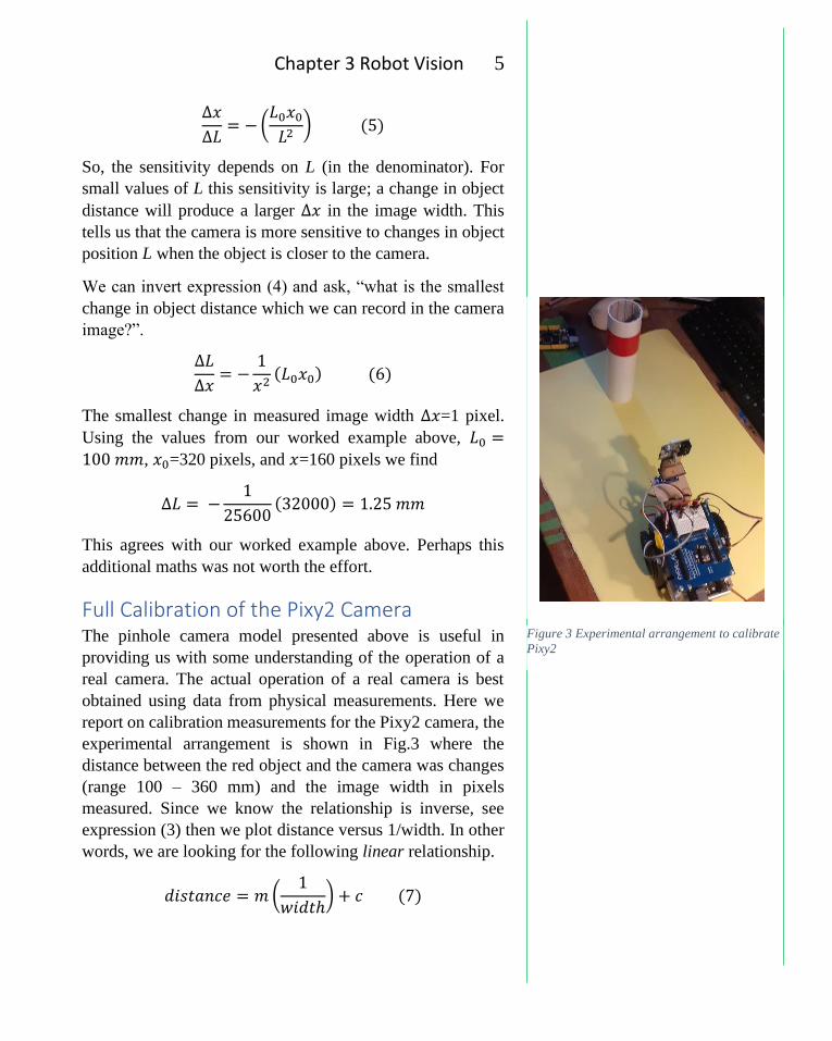
Figure 3 Experimental arrangement to calibrate

Pixy2

∆𝑥

∆𝐿= − (

𝐿0𝑥0

𝐿2) (5)

So, the sensitivity depends on L (in the denominator). For

small values of L this sensitivity is large; a change in object

distance will produce a larger ∆𝑥 in the image width. This

tells us that the camera is more sensitive to changes in object

position L when the object is closer to the camera.

We can invert expression (4) and ask, “what is the smallest

change in object distance which we can record in the camera

image?”.

∆𝐿

∆𝑥= −

1

𝑥2(𝐿0𝑥0) (6)

The smallest change in measured image width ∆𝑥=1 pixel.

Using the values from our worked example above, 𝐿0 =

100 𝑚𝑚, 𝑥0=320 pixels, and 𝑥=160 pixels we find

∆𝐿 = −1

25600(32000) = 1.25 𝑚𝑚

This agrees with our worked example above. Perhaps this

additional maths was not worth the effort.

Full Calibration of the Pixy2 Camera The pinhole camera model presented above is useful in

providing us with some understanding of the operation of a

real camera. The actual operation of a real camera is best

obtained using data from physical measurements. Here we

report on calibration measurements for the Pixy2 camera, the

experimental arrangement is shown in Fig.3 where the

distance between the red object and the camera was changes

(range 100 – 360 mm) and the image width in pixels

measured. Since we know the relationship is inverse, see

expression (3) then we plot distance versus 1/width. In other

words, we are looking for the following linear relationship.

𝑑𝑖𝑠𝑡𝑎𝑛𝑐𝑒 = 𝑚 (1

𝑤𝑖𝑑𝑡ℎ) + 𝑐 (7)

Nature of Computing 6

where m is the gradient of the straight line, and c is the

intercept. Here’s some typical results. The gradient is

calculated as the length of the green arrow divided by the

length of the red arrow (in units shown) and the intercept is

the dist value where 1/width is zero on the plot

My estimates are: gradient = 15625, intercept = -40. So, the

approximate relationship between width and distance is

𝑑𝑖𝑠𝑡𝑎𝑛𝑐𝑒 = 15625 (1

𝑤𝑖𝑑𝑡ℎ) − 40 (8)

However, we can do better than that. We can input the

gradient and intercept estimates into a nonlinear regression

program, which fits the curve to the data automatically, and

gives us the optimal values for gradient and intercept.

Automatic Non-Linear fitting This was done using the Octave script PixyDist.m which

makes use of the function nlinfit. You need to provide a data

set and a model to this function, here our model is the inverse

relation between width and distance. The syntax for the

model is

@(p,w) (p(1)./w) + p(2) (9)

Chapter 3 Robot Vision 7

The @(p,w) tells us that a function of variable w will follow

where p are the parameters to be fit by the function. Running

the script yields the following output

estimated parameters 15276.4 -38.3

95% confidence intervals 14606.6 to 15946.1 -51.5 to -25.1

r2 value 0.9966

The r2 value tells us that 99.7% of the data is explained by

the fitted curve. The confidence intervals are fine, though the

range for the second parameter is perhaps a little large. Our

manual fit was not bad at all! The final relationship between

width (pixels) and distance (mm) is therefore

𝑑𝑖𝑠𝑡 = 15276.7

𝑤𝑖𝑑𝑡ℎ− 38.3 (10)

We can use expression (9) in our code. Just for complete-

ness, here’s the non-linear fit curve.

This non-linear curve fitting is a useful skill to have for other

work. Now we can use the above values and write a function

to convert image width to distance.

float getDistanceFromObject(uint16_t width) {

float dist;

dist = gradient/(float)width + intercept;

return dist;

}

Figure 4 Robot moving through a cluttered

environment, needs to localize each object so it

can navigate between them.

Nature of Computing 8

Figure 6 Field of view of a camera, only

objects B and C are perceived

We have managed to write a computational function which

captures the workings of the camera based on experimental

data.

Application – Object Localization Object localization is more than object detection. In a

detection situation, we are content with detecting that the

robot is about to collide with something, so we can avoid it.

Localization is more precise; when a robot localizes an object

it finds out where it is (relative to its own location), in other

words, it must find the angle of the object and the distance to

the object.

When a robot moves in a cluttered environment (Fig.4) it

needs to know where the objects are located. How it does this

depends on its sensors. If it has a laser sensor, which sends

out a ray which collides with an object, then it is clear that it

needs to scan the space it is moving into. This means rotating

the laser ray from 0 to 180 degrees (looking forward) and

sensing any object at any angle. This is shown in Fig. 5.

But when the robot has a camera, it may not need to do this

scanning, since the camera captures objects within its field of

view. The robot could simply analyze what it sees and based

on this it would decide how to move.

Figure 6 shows such a scenario. Consider the case of a single

object in the camera’s field of view. The Pixycam can tell us

the x-location of the object (measured horizontally from the

left image boundary) and we can use this to generate an error

signal to drive the robot wheels to move the object towards

the centre of the FOV. This is shown in Fig.7 where the object

is to the right of centre, so the robot has rotated clockwise in

order to centre the object

If the camera is pointing forward, then the object is in the

correct place when it is at the centre of the image; here there

Figure 5 Robot scanning an environment.

Top, scans, middle, finds an object at 110

degrees, bottom rotates to face the object

ready for the kill

Chapter 3 Robot Vision 9

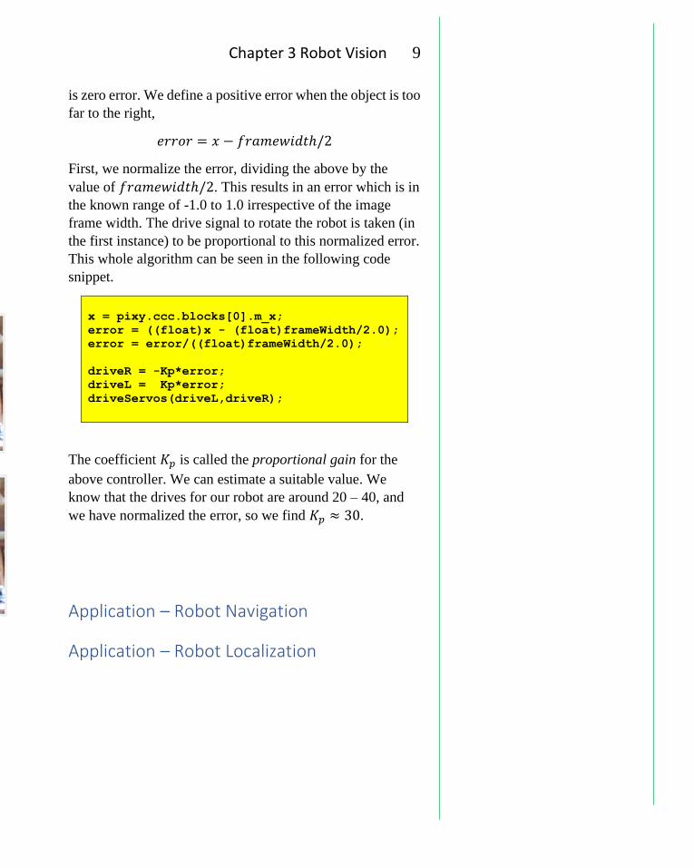
is zero error. We define a positive error when the object is too

far to the right,

𝑒𝑟𝑟𝑜𝑟 = 𝑥 − 𝑓𝑟𝑎𝑚𝑒𝑤𝑖𝑑𝑡ℎ/2

First, we normalize the error, dividing the above by the

value of 𝑓𝑟𝑎𝑚𝑒𝑤𝑖𝑑𝑡ℎ/2. This results in an error which is in

the known range of -1.0 to 1.0 irrespective of the image

frame width. The drive signal to rotate the robot is taken (in

the first instance) to be proportional to this normalized error.

This whole algorithm can be seen in the following code

snippet.

x = pixy.ccc.blocks[0].m_x;

error = ((float)x - (float)frameWidth/2.0);

error = error/((float)frameWidth/2.0);

driveR = -Kp*error;

driveL = Kp*error;

driveServos(driveL,driveR);

The coefficient 𝐾𝑝 is called the proportional gain for the

above controller. We can estimate a suitable value. We

know that the drives for our robot are around 20 – 40, and

we have normalized the error, so we find 𝐾𝑝 ≈ 30.

Application – Robot Navigation

Application – Robot Localization

Nature of Computing 10

Chapter 3 Robot Vision 11

Nature of Computing 12