Chapter -3 RESULTS AND DISCSSION -...
15
56 Chapter -3 RESULTS AND DISCSSION 3.1. INTRODUCTION In nanotechnology, an iron oxide nanoparticle, is defined as a small object that behaves as a whole unit in terms of its transport and properties. Particles are further classified according to size: in terms of diameter, fine particles cover a range between 100 and 2500nanometers. On the other hand, ultrafine particles are sized between 1 and 100nanometers. Similar to ultrafine particles, nanoparticles are sized between 1 and 100nanometers. Nanoparticles may or may not exhibit size-related properties that differ significantly from those observed in fine particles or bulk materials (Buzea et al., 2007). Iron oxides are chemical compounds composed of iron and oxygen. Altogether, there are sixteen known iron oxides and oxyhydroxides (Cornell & Schwertmann, 2003). The uses of these various oxides and hydroxides are tremendously diverse ranging from pigments in ceramic glaze, to use in thermite. Iron (III) oxide or ferric oxide is the inorganic compound with the formula Fe 2 O 3 . It is of one of the three main oxides of iron, the other two being iron(II) oxide (FeO), which is rare, and iron(II,III) oxide (Fe 3 O 4 ), which also occurs naturally as the mineral magnetite. As the mineral known as hematite, Fe 2 O 3 is the main source of the iron for the steel industry. Fe 2 O 3 is paramagnetic, reddish brown, and readily attacked by acids. Rust is often called iron (III) oxide and to some extent, this label is useful, because rust shares several properties and has a similar composition. In the present research work an emphasis has been made to focus on the synthesis of the iron oxide nano particles, subsequently which were used for the treatment of MSW by stabilizing process. Before the use of nano particle, they were characterized by XRD, XRF and SEM techniques. The presences of the functional group in iron oxide nano particle were characterized through XRF techniques and SEM was carried to determine the surface feature of the nano particle. Cadmium, Copper, Lead, Chromium and Mercury are the five Heavy metals considered for MSW samples and Bottom ash samples.
Transcript of Chapter -3 RESULTS AND DISCSSION -...

56
Chapter -3
RESULTS AND DISCSSION
3.1. INTRODUCTION
In nanotechnology, an iron oxide nanoparticle, is defined as a small object that
behaves as a whole unit in terms of its transport and properties. Particles are further
classified according to size: in terms of diameter, fine particles cover a range between
100 and 2500nanometers. On the other hand, ultrafine particles are sized between 1
and 100nanometers. Similar to ultrafine particles, nanoparticles are sized between 1
and 100nanometers. Nanoparticles may or may not exhibit size-related properties that
differ significantly from those observed in fine particles or bulk materials (Buzea et
al., 2007).
Iron oxides are chemical compounds composed of iron and oxygen.
Altogether, there are sixteen known iron oxides and oxyhydroxides (Cornell &
Schwertmann, 2003). The uses of these various oxides and hydroxides are
tremendously diverse ranging from pigments in ceramic glaze, to use in thermite. Iron
(III) oxide or ferric oxide is the inorganic compound with the formula Fe2O3. It is of
one of the three main oxides of iron, the other two being iron(II) oxide (FeO), which
is rare, and iron(II,III) oxide (Fe3O4), which also occurs naturally as the mineral
magnetite. As the mineral known as hematite, Fe2O3 is the main source of the iron for
the steel industry. Fe2O3 is paramagnetic, reddish brown, and readily attacked by
acids. Rust is often called iron (III) oxide and to some extent, this label is useful,
because rust shares several properties and has a similar composition.
In the present research work an emphasis has been made to focus on the
synthesis of the iron oxide nano particles, subsequently which were used for the
treatment of MSW by stabilizing process. Before the use of nano particle, they were
characterized by XRD, XRF and SEM techniques. The presences of the functional
group in iron oxide nano particle were characterized through XRF techniques and
SEM was carried to determine the surface feature of the nano particle. Cadmium,
Copper, Lead, Chromium and Mercury are the five Heavy metals considered for
MSW samples and Bottom ash samples.
57
0
1000
2000
3000
4000
5000
6000
0 10 20 30 40 50 60 70
INTENSITY
2θ
Fe2O3
Fe2O3
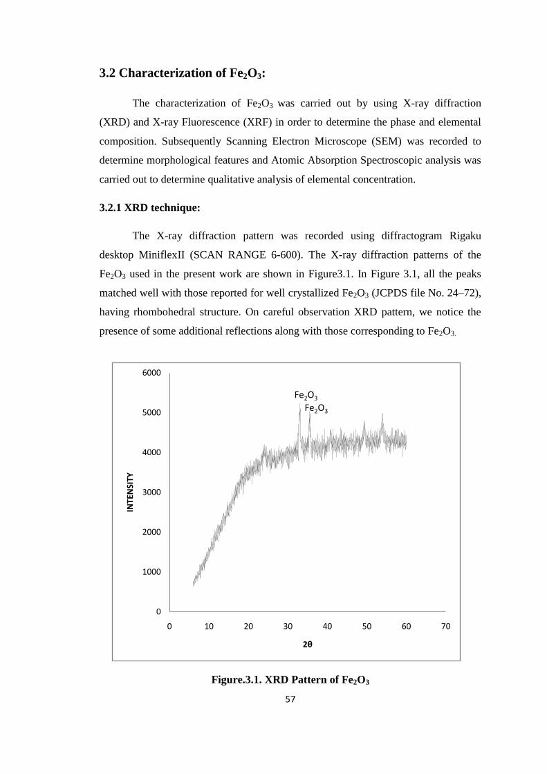
3.2 Characterization of Fe2O3:
The characterization of Fe2O3 was carried out by using X-ray diffraction
(XRD) and X-ray Fluorescence (XRF) in order to determine the phase and elemental
composition. Subsequently Scanning Electron Microscope (SEM) was recorded to
determine morphological features and Atomic Absorption Spectroscopic analysis was
carried out to determine qualitative analysis of elemental concentration.
3.2.1 XRD technique:
The X-ray diffraction pattern was recorded using diffractogram Rigaku
desktop MiniflexII (SCAN RANGE 6-600). The X-ray diffraction patterns of the
Fe2O3 used in the present work are shown in Figure3.1. In Figure 3.1, all the peaks
matched well with those reported for well crystallized Fe2O3 (JCPDS file No. 24–72),
having rhombohedral structure. On careful observation XRD pattern, we notice the
presence of some additional reflections along with those corresponding to Fe2O3.
Figure.3.1. XRD Pattern of Fe2O3

58
3.2.2. XRF Analysis:
X-ray fluorescence spectrum was recorded using Minipal- 4 benchtop model,
with fine focus x-ray tube, MO target of multilayer monochromator of 17.5KeV. The
XRF spectra of Fe2O3 clearly indicate that the presence of Fe+3
(Figure 3.2).
Figure.3.2. XRF Spectra of Fe2O3

59
3.2.3 Scanning Electron Microscopy (SEM):
The SEM images were taken by using Scanning electron microscope (Model
EOV LS 15). The surface morphologies of the Fe2O3 were observed by scanning
electron micrographic images as shown in Figure 3.3. SEM image can clearly shows
the particles having various shapes and also estimation of the particle size appeared
very difficult for the samples reported herein specially because of their extremely
small dimension and inherent nature of agglomeration which is obvious due to high
dipole interactions.
Figure.3.3. SEM image of Fe2O3

60
0
500
1000
1500
2000
2500
3000
3500
4000
0 10 20 30 40 50 60 70
INTENSITY
2θ
FeOOH FeOOH
3.3. Characterization of FeOOH
The characterization of FeOOH was carried out by using X-ray diffraction
(XRD) and X-ray Fluorescence (XRF) in order to determine the phase and elemental
composition. Subsequently Scanning Electron Microscope (SEM) was recorded to
determine morphological features and Atomic Absorption Spectroscopic analysis was
carried out to determine qualitative analysis of elemental concentration.
3.3.1. XRD technique:
The X-ray diffraction patterns of the FeOOH used in the present work are
shown in Figure3.4. In Figure 3.4, the identification of crystalline phase of FeOOH
was accomplished by comparison with JCPDS file No. 29–0713. On careful
observation XRD pattern, we notice the presence of some additional reflections along
with those corresponding to FeOOH.
Figure.3.4.XRD Pattern of FeOOH

61
3.3.2. XRF Analysis:
X-ray fluorescence spectrum was recorded using Minipal- 4 benchtop model,
with fine focus X-ray tube, MO target of multilayer monochromator of 17.5KeV.
Figure.3.5 clearly indicates that the pattern shows the presence the Fe+2
.
Figure.3.5. XRF Spectra of FeOOH
62
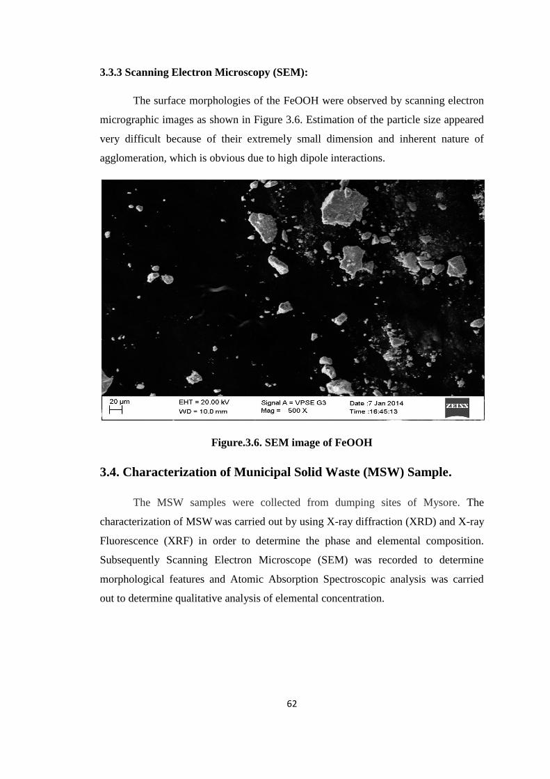
3.3.3 Scanning Electron Microscopy (SEM):
The surface morphologies of the FeOOH were observed by scanning electron
micrographic images as shown in Figure 3.6. Estimation of the particle size appeared
very difficult because of their extremely small dimension and inherent nature of
agglomeration, which is obvious due to high dipole interactions.
Figure.3.6. SEM image of FeOOH
3.4. Characterization of Municipal Solid Waste (MSW) Sample.
The MSW samples were collected from dumping sites of Mysore. The
characterization of MSW was carried out by using X-ray diffraction (XRD) and X-ray
Fluorescence (XRF) in order to determine the phase and elemental composition.
Subsequently Scanning Electron Microscope (SEM) was recorded to determine
morphological features and Atomic Absorption Spectroscopic analysis was carried
out to determine qualitative analysis of elemental concentration.

63
0
200
400
600
800
1000
1200
1400
0 10 20 30 40 50 60 70
INTENSITY
2θ
1
4 35
26
1= Ca(OH)2
2=Hg3=NaCl4=Cd5=Pb
6=Cr
3.4.1. X-Ray Diffraction analysis of MSW
X-ray Diffraction spectra of Municipal Solid Waste (MSW) are shown in
Figure 3.7. The reflection of heavy metal peaks were match through Crystal Impact
software (Match copy right 2003-2014), Bonn, Germany. The diffractogram of MSW
clearly indicate the presence of heavy metal like Cadmium, Copper, Lead, Mercury
and Chromium were present in the sample.
Figure.3.7. XRD pattern of MSW sample
3.4.2 XRF Analysis:
Elemental compositions of MSW samples have been analyzed using the X-ray
fluorescence technique. Figure 3.8 shows the XRF pattern of MSW sample. It was
observed that in MSW samples, concentration levels of all the elements are higher
than the ecological screening values and in case of Fe and Ca concentration is more
when compare to other elements. It is well known that traces of Cu, Zn, Mn, Cr, Mo,

64
Co, etc., are very essential for human bodies but higher doses and accumulation of
these elements might cause adverse effects in the body.
Figure.3.8. XRF Spectra of MSW sample

65
3.4.3. Scanning Electron Microscopy (SEM):
SEM image of MSW sample is shown in Figure 3.9. The collected material
was taken under the SEM without any treatment. Observing the SEM it looks bit
porous in nature. It is observed that the material looks more coiled and bit clustered
on the surface may due to the presence of high amount of organic materials along
with inorganic and heavy metals.
Figure. 3.9. SEM image of MSW sample

66
3.4.4. AAS analysis for MSW:
MSW was analysed for heavy metals by Atomic absorption spectroscopy. The
analysis shows that sample was rich in copper content 1.158 mg/kg compared to other
heavy metals. Metals such as Chromium 0.315 mg/kg and lead 0.257 mg/kg were
found at lower concentrations whereas cadmium and mercury concentration was
found to be 0.001 mg/kg. This study is well match with XRF study. Table 3.1 shows
the concentration of selected five heavy metals concentration.
Table.3.1. Heavy metal concentrations for the MSW samples
Sl.No Heavy Metal Concentration (mg/kg)
1 Cadmium <0.001
2 Copper 1.158
3 Lead 0.257
4 Chromium 0.315
5 Mercury <0.001
3.5. Characterization of Steel Bottom ash (BA) sample.
The Bottom Ash samples were collected from dumping sites of VISL,
Bhadravathi. The characterization of Bottom Ash was carried out by using X-ray
diffraction (XRD) and X-ray Fluorescence (XRF) in order to determine the phase and
elemental composition. Subsequently Scanning Electron Microscope (SEM) was
recorded to determine morphological features and Atomic Absorption Spectroscopic
analysis was carried out to determine qualitative analysis of elemental concentration.

67
0
500
1000
1500
2000
2500
3000
3500
4000
4500
0 10 20 30 40 50 60 70
INTENSITY
2θ
1=Fe
2=Ca3=Mn4=Cu5=Hg6=Si
1
2 35
46
3.5.1. X-Ray Diffraction analysis of Bottom ash.
The X-ray diffraction pattern of Bottom ash used in the present work is shown
in Figure 3.10. The XRD pattern of Bottom ash represent the presence of Heavy
metals and heavy metals peaks are shown in Figure 3.10. The peaks correspond to
heavy metal match was made through Crystal Impact software (Match copy right
2003-2014), Bonn, Germany. The study of XRD pattern clearly indicates that the
presence Cadmium, Copper, Lead, Mercury and Chromium particles are present in the
sample.
Figure 3.10. XRD Pattern of Bottom ash sample

68
3.5.2 XRF Analysis:
Elemental compositions of Bottom ash sample have been analyzed using the
X-ray fluorescence technique as shown in Figure 3.11. The samples were collected
from dumping sites of VISL, Bhadravathi. It was observed that in Bottom ash sample,
presence of Copper, Lead, and Mercury particles.
Figure 3.11. XRF Spectra of Bottom ash sample

69
3.5.3 Scanning Electron Microscopy (SEM):
SEM image of Bottom ash sample is shown in figure 3.13. The collected
material was taken under the SEM without any further treatment. The SEM studies
showed that the particles had subrounded to angular shapes. Distinct edges were
visible in angular, bulky particles. The gravel-size particles had shapes varying from
sub rounded to sub angular. Distinct edges were visible in sub angular, bulky
particles. Most of the particles had a high spherical and a solid structure. A
heterogeneous porous structure was also observed on the surface of a few particles.
Figure 3.12. SEM Picture of Bottom ash sample
3.5.4 AAS Analysis for Bottom ash sample:
Bottom ash sample was analysed for heavy metals by using Atomic absorption
spectroscopy, which shows that sample was rich in Chromium 0.427 mg/kg compared
to other heavy metals. Metals such as copper content 0.251 mg/kg and lead 0.041
mg/kg were found at lower concentrations whereas cadmium and mercury
concentration was found to be 0.001 mg/kg. Table 3.2 shows the concentration of
selected five heavy metals concentration.

70
Table.3.2. Heavy metal concentration in Bottom ash sample
Sl.No Heavy metals Concentration (mg/kg)
1 Cadmium <0.001
2 Copper 0.251
3 Lead 0.041
4 Chromium 0.427
5 Mercury <0.001