Chapter 3 Properties of a pure substance -...
36
Chapter 3 Properties of a pure substance Read BS, Chapter 3 3.1 The pure substance We define a • Pure substance: a material with homogeneous and invariable composition. To elaborate, • Pure substances can have multiple phases: an ice-water mixture is still a pure sub- stance. • An air-steam mixture is not a pure substance. • Air, being composed of a mixture of N 2 , O 2 , and other gases, is formally not a pure substance. However, experience shows that we can often treat air as a pure substance with little error. 3.2 Vapor-liquid-solid phase equilibrium Often we find that different phases of pure substances can exist in equilibrium with one another. Let us consider an important gedankenexperiment (Latin-German for “thought experiment”) in which we boil water. Ordinary water boiling is shown in Fig. 3.1. However, this ordinary experiment has constraints which are too loose. Most importantly, the mass of water leaks into the atmosphere; thus, the water vapor and the air become a mixture and no longer a pure substance. Let us instead consider a more controlled piston-cylinder arrangement. Inside the cylin- der, we begin with pure liquid water at T = 20 ◦ C . The piston is free to move in the cylinder, but it is tightly sealed, so no water can escape. On the other side of the piston is a constant pressure atmosphere, which we take to be at P = 100 kPa =0.1 MPa = 10 5 Pa =1 bar. 43
Transcript of Chapter 3 Properties of a pure substance -...
Chapter 3
Properties of a pure substance
Read BS, Chapter 3
3.1 The pure substance
We define a
• Pure substance: a material with homogeneous and invariable composition.
To elaborate,
• Pure substances can have multiple phases: an ice-water mixture is still a pure sub-stance.
• An air-steam mixture is not a pure substance.
• Air, being composed of a mixture of N2, O2, and other gases, is formally not a puresubstance. However, experience shows that we can often treat air as a pure substancewith little error.
3.2 Vapor-liquid-solid phase equilibrium
Often we find that different phases of pure substances can exist in equilibrium with oneanother. Let us consider an important gedankenexperiment (Latin-German for “thoughtexperiment”) in which we boil water. Ordinary water boiling is shown in Fig. 3.1. However,this ordinary experiment has constraints which are too loose. Most importantly, the massof water leaks into the atmosphere; thus, the water vapor and the air become a mixture andno longer a pure substance.
Let us instead consider a more controlled piston-cylinder arrangement. Inside the cylin-der, we begin with pure liquid water at T = 20 ◦C. The piston is free to move in the cylinder,but it is tightly sealed, so no water can escape. On the other side of the piston is a constantpressure atmosphere, which we take to be at P = 100 kPa = 0.1 MPa = 105 Pa = 1 bar.
43

44 CHAPTER 3. PROPERTIES OF A PURE SUBSTANCE
Figure 3.1: Water boiling isobarically in an open environment.
We slowly add heat to the cylinder, and observe a variety of interesting phenomena. A sketchof what we observe is given in Fig. 3.2. We notice the following behavior:
P = 100 kPa
liquid water T = 20 oC
P = 100 kPa
liquid waterT > 20 oC
P = 100 kPa
saturatedliquid waterT = 99.62 oC
P = 100 kPa
liquid,T = 99.62 oC
P = 100 kPa
saturatedwater vaporT = 99.62 oC
Q
P = 100 kPa
water vaporT > 99.62 oC
Q Q Q Q
vapor,T=99.62 oC
Figure 3.2: Sketch of experiment in which heat is added isobarically to water in a closedpiston-cylinder arrangement.
• The pressure remains at a constant value of 100 kPa. This is an isobaric process.
• The total volume increases slightly as heat is added to the liquid.
• The temperature of the liquid increases significantly as heat is added to the liquid.
• At a special value of temperature, observed to be T = 99.62 ◦C, we have all liquid, butcannot add any more heat and retain all liquid. We will call this state the saturatedliquid state. We call T = 99.62 ◦C the saturation temperature at P = 100 kPa. As wecontinue to add heat,
CC BY-NC-ND. 09 May 2013, J. M. Powers.
3.2. VAPOR-LIQUID-SOLID PHASE EQUILIBRIUM 45
– The temperature remains constant (this is isothermal now as well as isobaric).
– The total volume continues to increase.
– We notice two phases present: liquid and vapor, with a distinct phase boundary.The liquid is dense relative to the vapor. That is ρf > ρg, where f denotes fluidor liquid and g denotes gas or vapor. Thus, vg > vf .
– As more heat is added, more vapor appears, all while P = 100 kPa and T =99.62 ◦C.
– At a certain volume, we have all vapor and no liquid, still at P = 100 kPa,T = 99.62 ◦C. We call this state the saturated vapor state.
• As heat is added, we find both the temperature and the volume rise, with the pressureremaining constant. The water remains in the all vapor state.
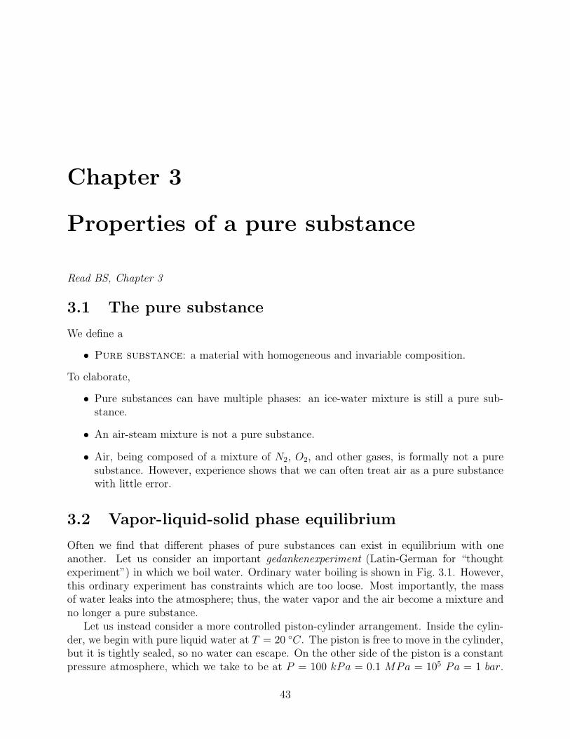
We have just boiled water! We sketch this process in the temperature-specific volume plane,that is, the T − v plane, in Fig. 3.3. Note that the mass m of the water is constant in this
v
T
two-phasemixture
vf
vg
P
= 100
kPa (iso
bar)
saturatedliquid saturated
vapor
Figure 3.3: Isobar in the T − v plane for our thought experiment in which heat is addedisobarically to water in a piston-cylinder arrangement.
problem, so the extensive V is strictly proportional to specific volume, v = V/m.We next repeat this experiment at lower pressure (such as might exist on a mountain
top) and at a higher pressure (such as might exist in a valley below sea level). For moderatepressures, we find qualitatively the exact same type of behavior. The liquid gets hotter,turns into vapor isothermally, and then the vapor gets hotter as the heat is added. However,we note the following important facts:
• The saturation temperature (that is the boiling point) increases as pressure increases,as long as the pressure increase is not too high.
CC BY-NC-ND. 09 May 2013, J. M. Powers.

46 CHAPTER 3. PROPERTIES OF A PURE SUBSTANCE
• As pressure increases vf becomes closer to vg.
• Above a critical pressure, P = Pc = 22.089 MPa, there is no phase change ob-served!1 At the critical pressure, the temperature takes on a critical temperature ofTc = 374.14 ◦C. At the critical pressure and temperature, the specific volume takes thevalue vf = vg = vc = 0.003155 m3/kg.
We see how the boiling point changes with pressure by plotting the saturation pressureas a function of saturation temperature in the T − P plane in Fig. 3.4. This is the so-calledvapor pressure curve. Here, we focus on liquid-vapor mixtures and keep T high enough to
T
P
superheatedvapor
compressedliquid
criticalpoint
Tc
Pc
vapor
pressu
re cu
rve
Figure 3.4: Saturation pressure versus saturation temperature sketch.
prevent freezing. Note the curve terminates abruptly at the critical point.We adopt the following nomenclature:
• saturated liquid: the material is at Tsat and is all liquid.
• saturated vapor: the material is at Tsat and is all vapor.
• compressed (subcooled) liquid: the material is liquid with T < Tsat.
• superheated vapor: the material is vapor with T > Tsat.
• two-phase mixture: the material is composed of co-existing liquid and vapor withboth at Tsat.
1This behavior may have first been carefully documented by T. Andrews, 1869, “The Bakerian lecture:on the continuity of the gaseous and liquid states of matter,” Philosophical Transactions of the Royal Society
of London, 159: 575-590.
CC BY-NC-ND. 09 May 2013, J. M. Powers.

3.2. VAPOR-LIQUID-SOLID PHASE EQUILIBRIUM 47
For two-phase mixtures, we define a new property to characterize the relative concentra-tions of liquid and vapor. We define the
• quality= x: as the ratio of the mass of the mixture which is vapor (vap) to the totalmixture mass:
x =mvap
mtotal. (3.1)
We can also take the total mass to be the sum of the liquid and vapor masses:
mtotal = mliq +mvap. (3.2)
Sox =
mvap
mliq +mvap. (3.3)
There are two important limits to remember:
• x = 0: corresponds to mvap = 0. This is the all liquid limit.
• x = 1: corresponds to mvap = mtotal. This is the all gas limit.
We must have0 ≤ x ≤ 1. (3.4)
We sketch water’s T − v plane again for a wide variety of isobars in Fig. 3.5. We sketch
v
T
saturated vapor linesaturated
liquid line
superheatedvapor
two-phasemixture
com
pre
ssed
liquid
criticalpoint
P = 0.1 MPa
Pc = 22.089 MPa
P = 10 MPa
P = 1 MPa
P = 40 MPa
Tc = 374.14 oC
T= 99.62 oC
vc = 0.003155 m3/kg
Figure 3.5: Sketch of T − v plane for water for a variety of isobars.
water’s P − v plane for a wide variety of isotherms in Fig. 3.6. We can perform a similarthought experiment for ice. We can start with ice at P = 100 kPa and add heat to it. We
CC BY-NC-ND. 09 May 2013, J. M. Powers.

48 CHAPTER 3. PROPERTIES OF A PURE SUBSTANCE
v
P
saturated vapor line
saturated liquid line
superheatedvapor
two-phasemixture
com
pre
ssed
liquid
criticalpoint
Tlow
Thigh
Tc = 374.14
oC
Pc = 22.089 MPa
vc = 0.003155 m3/kg
Figure 3.6: Sketch of P − v plane for water for a variety of isotherms.
observe the ice’s temperature rise until T = Tsat ∼ 0 ◦C. At that temperature, the ice beginsto melt and the temperature remains constant until all the ice is melted. At this point theliquid temperature begins to rise. If we continued to add heat, we would boil the water.
We note if we perform this experiment for P < 0.6113 kPa the ice in fact goes directlyto vapor. It is said to have undergone sublimation. There exists a second important pointwhere ice being heated isobarically can transform into either liquid or gas. This is the so-called triple point. At the triple point we find the saturation pressure and temperature arePtp = 0.6113 kPa and Ttp = 0.01 ◦C, respectively. It is better described as a triple line,because in the P −v−T space we will study, it appears as a line with constant P and T , butvariable v. In the P −T projected plane of the P − v−T volume, it projects as a point. Wesketch water’s P − T plane again for a wider range to include the vapor-liquid-solid phasebehavior in Fig. 3.7.
These characteristics apply to all pure substances. For example, nitrogen has a triplepoint and a critical point. Table A.2 in BS lists critical constants for many materials. Notealso that phase transitions can occur within solid phases. This involves a re-arrangement ofthe crystal structure. This has important implications for material science, but will not beconsidered in detail in this course.
3.3 Independent properties
Let us define a
• Simple compressible substance: a material that can be worked upon by pressureforces.
CC BY-NC-ND. 09 May 2013, J. M. Powers.

3.4. THERMAL EQUATIONS OF STATE 49
T(oC)
P(kPa)
superheatedvapor
compressedliquid
criticalpoint
solid
triplepoint
vapo
rizat
ion
line
sublim
ation
line
supercriticalfluid
0.01
0.6113
22089
374.14
fusion
lin
e
Figure 3.7: Sketch of P − T plane for water.
Note we neglect electric, magnetic, and chemical work modes. While this is indeed restrictive,it will be important for many mechanical engineering applications. The following importantstatement can be proved (but will not be so here):
• For a simple compressible substance, two independent intensive thermodynamic prop-erties define the state of the system.
Consider the implications for
• superheated vapor: If we consider P , T , and v, this states that we must allow one of thevariables to be functions of the other two. We could have P = P (T, v), v = v(T, P ),or T = T (P, v). All are acceptable.
• two-phase mixture: If we have a two-phase mixture, our experiments show that P andT are not independent. In this case, we need another property to characterize thesystem. That property is the quality, x. So for two-phase mixtures, we might havev = v(T, x), for example.
3.4 Thermal equations of state
Here, we will describe some of the many different ways to capture the relation between twoindependent properties and a third dependent property for a simple compressible substance.We will focus on a so-called
CC BY-NC-ND. 09 May 2013, J. M. Powers.

50 CHAPTER 3. PROPERTIES OF A PURE SUBSTANCE
• Thermal equation of state: an equation which gives the pressure as a functionof two independent state variables. An example is the general form:
P = P (T, v). (3.5)
We will progress from simple thermal equations of state to more complex.
3.4.1 Ideal gas law
For many gases, especially at low density and far from the critical point, it is possible towrite a simple thermal equation of state which accurately describes the relation betweenpressure, volume, and temperature. Such equations were developed in the 1600s and early1800s based entirely on macroscopic empirical observation. In the late 1800s, statisticalmechanics provided a stronger theoretical foundation for them, but we will not consider thathere.
Let us start with the most important equation of state:
• Ideal gas law: This equation, which is a combination of Boyle’s law,2 Charles’ law,3
and Avogadro’s law,4 is most fundamentally stated as
PV = nRT. (3.6)
On the continent, Boyle’s law is sometimes known as Mariotte’s law after Edme Mariotte(1620-1684), but Boyle published it fourteen years earlier.5 A reproduction of Boyle’s datais given in Fig. 3.8.6 The data in (V, 1/P ) space is fit well by a straight line with interceptat the origin; that is 1/P = KV , where K is a constant. Thus, PV = C, where C = 1/K isa constant.
2R. Boyle, 1662, New Experiments Physico-Mechanical, Touching the Air: Whereunto is Added A Defence
of the Authors Explication of the Experiments, Against the Obiections of Franciscus Linus and Thomas
Hobbes, H. Hall, Oxford. There exists a 1725 text modified from the 1662 original in The Philosophical
Works of Robert Boyle, Vol. 2, P. Shaw, ed., Innis, Osborn, and Longman, London. Boyle’s law holds thatPV is constant in an isothermal process.
3attributed to J. A. C. Charles by J. L. Gay-Lussac, 1802, “Recherches sur la dilatation des gaz desvapeurs,” Annales de Chimie, 43(1): 137-175. Charles’ law holds that V/T is constant for ideal gasesundergoing isobaric processes. Additionally, Guillaume Amontons (1663-1705) performed some of the earlyexperimentation which led to Charles’ law. John Dalton (1766-1844) is said to have also written on a versionof Charles’ Law in 1801.
4A. Avogadro, 1811, “Essai d’une maniere de determiner les masses relatives des molecules elementairesdes corps, et les proportions selon lesquelles elles entrent dans ces combinaisons,” Journal de Physique,
de Chimie et d’Historie Naturelle, 73:58-76. Here, Avogadro hypothesized that “equal volumes of ideal orperfect gases, at the same temperature and pressure, contain the same number of particles, or molecules.”
5C. Webster, 1965, “The discovery of Boyle’s law, and the concept of the elasticity of air in the seventeenthcentury,” Archive for History of Exact Sciences, 2(6): 441-502. Also described here is how Henry Power(1623-1668) and Richard Towneley (1629-1707) did important preliminary work which helped Boyle formulatehis law.
6see J. B. West, 1999, “The original presentation of Boyle’s law, Journal of Applied Physiology, 98(1):31-39.
CC BY-NC-ND. 09 May 2013, J. M. Powers.

3.4. THERMAL EQUATIONS OF STATE 51
0 10 20 30 40 50
0.01
0.02
0.03
0.04
V (in3)
1/P
(in H
g)-1
a)
b)
Figure 3.8: a) Boyle’s 1662 data to validate his law (PV is constant for an isothermalprocess), b) plot of Boyle’s data: V (column A) versus reciprocal of P (reciprocal of columnD), demonstrating its near linearity.
CC BY-NC-ND. 09 May 2013, J. M. Powers.

52 CHAPTER 3. PROPERTIES OF A PURE SUBSTANCE
Depictions of Boyle, Charles, and Avogadro are given in Fig. 3.9. The ideal gas law was
a) b) c)
Figure 3.9: b) Robert Boyle (1627-1691), Irish scientist who developed an important specialcase of the ideal gas law. Image from http://en.wikipedia.org/wiki/Robert Boyle, c)Jacques Alexandre Cesar Charles (1746-1823), French scientist credited in 1802 by JosephLouis Gay-Lussac (1778-1850) for developing an important special case of the ideal gaslaw in the 1780s. Image from http://en.wikipedia.org/wiki/Jacques Charles,a) Lorenzo Romano Amedeo Carlo Avogadro di Quarengna e di Cerroto(1776-1856), Italian physicist, nobleman, and revolutionary. Image fromhttp://en.wikipedia.org/wiki/Amedeo Avogadro.
first stated in the form roughly equivalent to Eq. (3.6) by Clapeyron,7 depicted in Fig. 3.10.
It is critical that the temperature here be the absolute temperature. For the originalargument, see Thomson.8 Here, n is the number of moles. Recall there are N = 6.02214179×10²³ molecules in amole, where N is Avogadro’s number. Also R is the universal gas constant.From experiment, it is determined to be
R = 8.314472kJ
kmole K. (3.7)
In this class the over bar notation will denote an intensive property on a per mole basis.Intensive properties without over bars will be on a per mass basis. Recall the mass-basis
7E. Clapeyron, 1834, “Memoire sur la puissance motrice de la chaleur,” Journal de l’Ecole Polytechnique,14: 153-190.
8W. Thomson, 1848, “On an absolute thermometric scale founded on Carnot’s theory of the motive powerof heat and calculated from Regnault’s observations, Proceedings of the Cambridge Philosophical Society,1(5): 66-71.
CC BY-NC-ND. 09 May 2013, J. M. Powers.
3.4. THERMAL EQUATIONS OF STATE 53
Figure 3.10: Benoıt Paul Emile Clapeyron (1799-1824), French engineer andphysicist who furthered the development of thermodynamics. Image fromhttp://en.wikipedia.org/wiki/Emile Clapeyron.
specific volume is v = V/m. Let us define the mole-based specific volume as
v =V
n. (3.8)
Thus, the ideal gas law can be represented in terms of intensive properties as
PV
n︸︷︷︸
=v
= RT, (3.9)
Pv = RT. (3.10)
There are other ways to write the ideal gas law. Recall the molecular mass M is themass in g of a mole of substance. More common in engineering, it is the mass in kg of akmole of substance. These numbers are the same! From chemistry, for example, we knowthe molecular mass of O2 is 32 g/mole = 32 kg/kmole. Symbolically, we can say that
M =m
n. (3.11)
Now, take the ideal gas law and divide by m:
PV = nRT, (3.12)
PV
m︸︷︷︸
=v
=n
m︸︷︷︸
=1/M
RT, (3.13)
Pv =R
M︸︷︷︸
≡R
T. (3.14)
Now, let us define
R ≡ R
M. (3.15)
CC BY-NC-ND. 09 May 2013, J. M. Powers.

54 CHAPTER 3. PROPERTIES OF A PURE SUBSTANCE
Let’s check the units:
[R] =kJ
kmole K
kmole
kg=
kJ
kg K. (3.16)
We have actually just lost some universality. Recall R is independent of material. But sinceeach different gas has a different M , then each gas will have its own R. These values forvarious gases are tabulated in Table A.5 of BS.
With this definition, the ideal gas law becomes
Pv = RT. (3.17)
This is the form we will use most often in this class. Note the useful fact that
Pv
T= R. (3.18)
Thus, if an ideal gas undergoes a process going from state 1 to state 2, we can safely say
P1v1
T1=P2v2
T2. (3.19)
Example 3.1Find R for air.
We can model air as a mixture of N2 and O2. Its average molecular mass is known from Table A.5of BS to be M = 28.97 kg/kmole. So R for air is
R =R
M=
8.3145 kJkmole K
28.97 kgkmole
= 0.287kJ
kg K. (3.20)
Consider some notions from algebra and geometry. The function f(x, y) = 0 describes acurve in the x− y plane. In special cases, we can solve for y to get the form y = y(x). Thefunction f(x, y, z) = 0 describes a surface in the x− y − z volume. In special cases, we cansolve for z to get z = z(x, y) to describe the surface in the x− y − z volume.
Example 3.2Analyze the surface described by f(x, y, z) = z2 − x2 − y2 = 0.
Here, we can solve for z exactly to get
z = ±√
x2 + y2. (3.21)
This surface is plotted in Fig. 3.11. We can also get three two-dimensional projections of this surfacein the x − y plane, the y − z plane, and the x − z plane. Orthographic projections of this surface areplotted in Fig. 3.12.
CC BY-NC-ND. 09 May 2013, J. M. Powers.

3.4. THERMAL EQUATIONS OF STATE 55
� -2
� -1
0
1
2
x
�-2
�
0
1
2
y
�-2
�-1
0
1
2
z
-1
Figure 3.11: The surface z2 − x2 − y2 = 0.
-1 0 1 2-2
-1
0
1
2
x
y
-2 -1 0 1 2-2
-1
0
1
2
-2 -1 0 1 2-2
-1
0
1
2
x y
zz
iso-z contours
iso-ycontours
iso-xcontours
-2
Figure 3.12: Contours of constant x, y and z in orthographic projection planes of the surfacez2 − x2 − y2 = 0.
CC BY-NC-ND. 09 May 2013, J. M. Powers.
56 CHAPTER 3. PROPERTIES OF A PURE SUBSTANCE
For the x − y plane we consider
zo = ±√
x2 + y2. (3.22)
for various values of zo. This yields a family of circles in this plane. For the y − z plane, we consider
xo = ±√
z2 − y2. (3.23)
This gives a family of hyperbolas. For real xo, we require z2 ≥ y2. For the z − x plane, we consider
yo = ±√
z2 − x2. (3.24)
This gives a similar family of hyperbolas. For real yo, we require z2 ≥ x2.
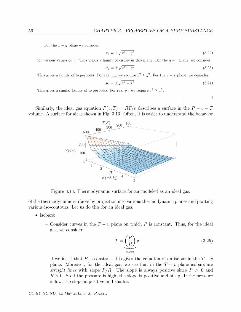
Similarly, the ideal gas equation P (v, T ) = RT/v describes a surface in the P − v − Tvolume. A surface for air is shown in Fig. 3.13. Often, it is easier to understand the behavior
100200300
400500
T(K)
12
34
5v (m3/kg)
0
100
200
P(kPa)
Figure 3.13: Thermodynamic surface for air modeled as an ideal gas.
of the thermodynamic surfaces by projection into various thermodynamic planes and plottingvarious iso-contours. Let us do this for an ideal gas.
• isobars:
– Consider curves in the T − v plane on which P is constant. Thus, for the idealgas, we consider
T =
(P
R
)
︸ ︷︷ ︸
slope
v. (3.25)
If we insist that P is constant, this gives the equation of an isobar in the T − vplane. Moreover, for the ideal gas, we see that in the T − v plane isobars arestraight lines with slope P/R. The slope is always positive since P > 0 andR > 0. So if the pressure is high, the slope is positive and steep. If the pressureis low, the slope is positive and shallow.
CC BY-NC-ND. 09 May 2013, J. M. Powers.

3.4. THERMAL EQUATIONS OF STATE 57
– Consider curves in the P − v plane in which P is constant. Thus, we consider
P = constant, (3.26)
which are straight horizontal lines in the P − v plane.
– Consider curves in the P − T plane in which P is a constant. Thus, we consider
P = constant, (3.27)
which are straight horizontal lines in the P − v plane.
Isobars in various planes are shown in Fig. 3.14.
v v T
T P PPhigh
Plow
Phigh
Plow
Phigh
Plow
Figure 3.14: Isobars for an ideal gas in T − v, P − v, and P − T planes.
• isotherms
– Consider curves in the T − v plane on which T is constant. Thus, for the idealgas, we have
T = constant (3.28)
These are straight horizontal lines in the T − v plane.
– Consider curves in the P − v plane on which T is a constant. Thus, for the idealgas, we have
P = (RT )1
v. (3.29)
These are hyperbolas in the P − v plane.
– Consider curves in the P − T plane on which T is a constant. Thus, for the idealgas, we have
T = constant. (3.30)
These are straight vertical lines in the P − T plane.
Isotherms in various planes are shown in Fig. 3.15.
CC BY-NC-ND. 09 May 2013, J. M. Powers.

58 CHAPTER 3. PROPERTIES OF A PURE SUBSTANCE
v v T
T P P
Thigh
Tlow
Thigh
Tlow
Thigh
Tlow
Figure 3.15: Isotherms for an ideal gas in T − v, P − v, and P − T planes.
• isochores
– Consider curves in the T − v plane on which v is constant. Thus, for the idealgas, we have
v = constant (3.31)
These are straight vertical lines in the T − v plane.
– Consider curves in the P − v plane on which v is a constant. Thus, for the idealgas, we have
v = constant. (3.32)
These are straight vertical lines in the P − v plane.
– Consider curves in the P − T plane on which v is a constant. Thus, for the idealgas, we have
P =
(R
v
)
︸ ︷︷ ︸
constant
T. (3.33)
These are straight lines in the P − T plane with slope R/v. Since R > 0 andv > 0, the slope is always positive. For large v, the slope is shallow. For small v,the slope is steep.
Isochores in various planes are shown in Fig. 3.16.
Example 3.3Given air in a cylinder with stops and a frictionless piston with area A = 0.2 m2, stop height of
1 m, and total height of 2 m, at initial state P1 = 200 kPa and T1 = 500 ◦C with cooling, find
• the temperature when the piston reaches the stops, and
• the pressure if the cooling continues to T = 20 ◦C.
CC BY-NC-ND. 09 May 2013, J. M. Powers.

3.4. THERMAL EQUATIONS OF STATE 59
v v T
T P Pvhigh
vlow
vhigh
vlowv
highv
low
Figure 3.16: Isochores for an ideal gas in T − v, P − v, and P − T planes.
1 m
1 m
air
A = 0.2 m2
Patm
A
PA
free body diagramat the initial state
Figure 3.17: Sketch for example problem of cooling air.
The initial state along with a free body diagram is sketched in Fig. 3.17.
We have three distinct states:
• state 1: initial state
• state 2: piston reaches the stops
• state 3: final state, where T = 20◦C.
At the initial state, the total volume is
V1 = A((1 m) + (1 m)) = (0.2 m2)(2 m) = 0.4 m3. (3.34)
We also know that P1 = 200 kPa. For use of the ideal gas law, we must use absolute temperature. So
T1 = 500 + 273.15 = 773.15 K. (3.35)
CC BY-NC-ND. 09 May 2013, J. M. Powers.
60 CHAPTER 3. PROPERTIES OF A PURE SUBSTANCE
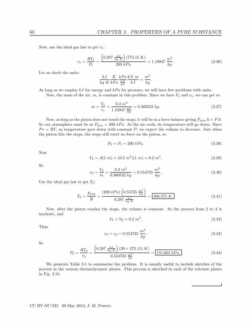
Now, use the ideal gas law to get v1:
v1 =RT1
P1=
(
0.287 kJkg K
)
(773.15 K)
200 kPa= 1.10947
m3
kg. (3.36)
Let us check the units:kJ
kg K
K
kPa
kPakNm2
kN m
kJ=
m3
kg.
As long as we employ kJ for energy and kPa for pressure, we will have few problems with units.Now, the mass of the air, m, is constant in this problem. Since we have V1 and v1, we can get m:
m =V1
v1=
0.4 m3
1.10947 m3
kg
= 0.360532 kg. (3.37)
Now, as long as the piston does not touch the stops, it will be in a force balance giving PatmA = PA.So our atmosphere must be at Patm = 200 kPa. As the air cools, its temperature will go down. SincePv = RT , as temperature goes down with constant P , we expect the volume to decrease. Just whenthe piston hits the stops, the stops still exert no force on the piston, so
P2 = P1 = 200 kPa. (3.38)
Now
V2 = A(1 m) = (0.2 m2)(1 m) = 0.2 m3. (3.39)
So
v2 =V2
m=
0.2 m3
0.360532 kg= 0.554735
m3
kg. (3.40)
Use the ideal gas law to get T2:
T2 =P2v2
R=
(200 kPa)(
0.55735 m3
kg
)
0.287 kJkg K
= 386.575 K. (3.41)
Now, after the piston reaches the stops, the volume is constant. So the process from 2 to 3 isisochoric, and
V3 = V2 = 0.2 m3. (3.42)
Thus
v3 = v2 = 0.554735m3
kg. (3.43)
So
P3 =RT3
v3=
(
0.287 kJkg K
)
(20 + 273.15) K)
0.554735 m3
kg
= 151.665 kPa. (3.44)
We generate Table 3.1 to summarize the problem. It is usually useful to include sketches of theprocess in the various thermodynamic planes. This process is sketched in each of the relevant planesin Fig. 3.18.
CC BY-NC-ND. 09 May 2013, J. M. Powers.

3.4. THERMAL EQUATIONS OF STATE 61
Table 3.1: Numerical values for ideal gas cooling example
variable units state 1 state 2 state 3T K 773.15 386.575 293.15P kPa 200 200 151.665
v m3
kg1.10947 0.554735 0.554735
V m3 0.4 0.2 0.2
v(m3/kg) v(m3/kg) T(K)
T(K) P(kPa) P(kPa)
200 - 200
151.6 - 151.6 -
773 -
386 -
293 -
1
2
3
12
3
12
3
0.555 1.11 0.555 1.11 386 773
T=293 K
T = 386 KT =
773 K
v = 1.11 m
3 /kg
P = 200
kPa
P = 15
1.6 kP
a v =
0.5
55 m
3 /kg
-
Figure 3.18: Sketch of T − v, P − v, and P − T planes for air-cooling example problem.
3.4.2 Non-ideal thermal equations of state
The ideal gas law is not a good predictor of the P − v − T behavior of gases when
• the gas has high enough density that molecular interaction forces become large andthe molecules occupy a significant portion of the volume; this happens near the vapordome typically, or
• the temperature is high enough to induce molecular dissociation (e.g. N2 + N2 ⇌
2N +N2)
One alternative is a corrected thermal equation of state.
3.4.2.1 van der Waals
For the van der Waals9 equation of state, which will be studied in more detail in Sec. 11.6,one has
P =RT
v − b− a
v2, (3.45)
9J. D. van der Waals, 1873, Over de Continuiteit van den Gas -en Vloeistoftoestand, Ph.D. Dissertation,U. Leiden; see also J. D. van der Waals, 1910, Nobel Lecture.
CC BY-NC-ND. 09 May 2013, J. M. Powers.

62 CHAPTER 3. PROPERTIES OF A PURE SUBSTANCE
with
a =27
64R2T
2c
Pc
, b =1
8RTc
Pc
. (3.46)
A depiction of van der Waals is given in Fig. 3.19.
Figure 3.19: Johannes Diderik van der Waals (1837-1923), Dutch physicistand Nobel laureate who developed a corrected state equation. Image fromhttp://en.wikipedia.org/wiki/Johannes Diderik van der Waals.
3.4.2.2 Redlich-Kwong
For the Redlich-Kwong10 equation of state, one has
P =RT
v − b− a
v(v + b)√T, (3.47)
with
a = (0.42748)R2T
5/2c
Pc
, b = (0.08664)RTc
Pc
. (3.48)
3.4.3 Compressibility factor
In some cases, more detail is needed to capture the behavior of the gas, especially near thevapor dome. Another commonly used approach to capturing this behavior is to define the
• Compressibility factor: the deviation from ideality of a gas as measured by
Z =Pv
RT. (3.49)
CC BY-NC-ND. 09 May 2013, J. M. Powers.

3.4. THERMAL EQUATIONS OF STATE 63
P (MPa)
2
1
01 10
300 K
130 K
200 K
saturated liquid
saturated vapor
criticalpoint
ideal gas, Z = 1
Z =
Pv/
RT
Figure 3.20: Sketch of compressibility chart for N2.
For ideal gases, Pv = RT , so Z = 1. Experiments show the behavior of real gases, and thiscan be presented in graphical form, as shown for N2 in Fig. 3.20. Note
• for all T , Z → 1 as P → 0. Thus, one has ideal gas behavior at low pressure
• for T > 300 K, Z ∼ 1 for P < 10 MPa.
• Hold at P = 4 MPa and decrease temperature from 300 K; we see Z decrease belowunity. Now
Z =Pv
RT=
P
ρRT, ρ =
P
ZRT. (3.50)
Since Z < 1, the density ρ is higher than we would find for an ideal gas with Z = 1.Thus, in this region, there is an attractive force between molecules.
• For P > 30 MPa, we find Z > 1. Thus, a repulsive force exists in this regime. Theforces are complicated.
Note that generalized compressibility charts have been developed for general gases. Theseare based on the so-called reduced pressures and temperatures, Pr and Tr, where
Pr =P
Pc
, Tr =T
Tc
. (3.51)
10O. Redlich and J. N. S. Kwong, 1949, “On the thermodynamics of solutions. V. an equation of state.fugacities of gaseous solutions,” Chemical Reviews, 44(1): 233-244.
CC BY-NC-ND. 09 May 2013, J. M. Powers.

64 CHAPTER 3. PROPERTIES OF A PURE SUBSTANCE
The reduced pressure and temperature are dimensionless. Values with the c subscript are thecritical constants for the individual gases. Appendix D of BS gives generalized compressibilitycharts.
3.4.4 Tabular thermal equations of state
Often equations are too inaccurate for engineering purposes. This is generally because wemay be interested in behavior under a vapor dome. Consider that the surface for steam iswell represented by that shown in Fig. 3.21.
Figure 3.21: P − v − T surface for H2O, showing solid, liquid, and vapor phases.
In such cases, one should use tables to find a third property, given two independentproperties. We can say that the thermal equation of state is actually embodied in thetabular data.
We lay down some rules of thumb for this class:
• If steam, use the tables.
• If air or most other gas, use the ideal gas law, but check if the pressure is high orthe properties are near the vapor dome, in which case use compressibility charts ornon-ideal state equations.
Let us look at how the tables are organized.
CC BY-NC-ND. 09 May 2013, J. M. Powers.

3.4. THERMAL EQUATIONS OF STATE 65
3.4.4.1 Saturated liquid-vapor water, temperature tables
For water, the most important table is the saturated steam table. One should go to suchtables first. If the water is a two-phase mixture, tables of this type must be used as theequation of state. Recall, for two-phase mixtures, pressure and temperature are not inde-pendent thermodynamic variables. Two properties still determine the state, but quality x isnow important. So for two-phase mixtures we allow
• T = T (v, x),
• P = P (v, x), or
• v = v(T, x),
for example. But P 6= P (T, v) as for ideal gases.
Consider the structure of saturation tables, as shown in Table 3.2, extracted from BS’sTable B.1.1. Data from the steam tables is sketched in Fig. 3.22. We have the notation:
Specific Volume, m3
kg
Temp. Press. Sat. Liquid Evap. Sat. Vapor◦C kPa vf vfg vg
0.01 0.6113 0.001000 206.131 206.1325 0.8721 0.001000 147.117 147.118
10 1.2276 0.001000 106.376 106.37715 1.705 0.001001 77.924 77.925
......
......
...35 5.628 0.001006 25.2148 25.215840 7.384 0.001008 19.5219 19.5229
......
......
...374.1 22089 0.003155 0 0.00315
Table 3.2: Saturated liquid-vapor water tables, temperature entry, from BS, Table B.1.1.
• f : saturated liquid,
• g: saturated vapor,
• vf : specific volume of saturated liquid, and
• vg: specific volume of saturated vapor.
CC BY-NC-ND. 09 May 2013, J. M. Powers.

66 CHAPTER 3. PROPERTIES OF A PURE SUBSTANCE
v(m3/kg )
T(oC)
compressedliquid
superheatedvapor
15 oC
vf=0.001000 m3/kg v
g =77.925 m3/kg
vfg = 77.924 m3/kg
f g
Figure 3.22: Vapor dome for H2O with data for vf , vg, and vfg at T = 15◦C.
Note for liquid-vapor mixtures, this table begins at the triple point temperature 0.01 ◦C andends at the critical temperature 374.1 ◦C. At P = Pc and T = Tc, we have vf = vg. Notethat
• vf ≃ constant
• vg decreases with increasing T
We define vfg as
vfg ≡ vg − vf . (3.52)
Recall the quality x is
x =mvap
mtotal.
Consider a mass of fluid m in total volume V . We must have
V = Vliq + Vvap, (3.53)
m = mliq +mvap. (3.54)
CC BY-NC-ND. 09 May 2013, J. M. Powers.

3.4. THERMAL EQUATIONS OF STATE 67
Now, use the definition of specific volume and analyze to get
mv = mliqvf +mvapvg, (3.55)
v =mliq
mvf +
mvap
mvg, (3.56)
v =m−mvap
mvf +
mvap
mvg, (3.57)
v = (1 − x)vf + xvg, (3.58)
v = vf + x (vg − vf )︸ ︷︷ ︸
=vfg
. (3.59)
We get the final important results:
v = vf + xvfg. (3.60)
x =v − vf
vfg
. (3.61)
3.4.4.2 Saturated liquid-vapor water, pressure tables
Sometimes we are given the pressure of the mixture, and a saturation table based on thepressure is more useful. An example of a portion of such a table is shown in Table 3.3.
Specific Volume, m3
kg
Press. Temp. Sat. Liquid Evap. Sat. VaporkPa ◦C vf vfg vg
0.6113 0.01 0.001000 206.131 206.1321.0 6.98 0.001000 129.20702 129.208021.5 13.03 0.001001 87.97913 87.980132.0 17.50 0.001001 67.00285 67.00385
......
......
...22089 374.1 0.003155 0 0.00315
Table 3.3: Saturated water tables, pressure entry from BS, Table B.1.2.
Example 3.4Given a vessel with V = 0.4 m3 filled with m = 2 kg of H2O at P = 600 kPa, find
• the volume and mass of liquid, and
• the volume and mass of vapor.
CC BY-NC-ND. 09 May 2013, J. M. Powers.

68 CHAPTER 3. PROPERTIES OF A PURE SUBSTANCE
liquid water
water vapor
P = 600 kPam = 2 kgV = 0.4 m3
Figure 3.23: Schematic for liquid-vapor mixture example problem.
The problem is sketched in Fig. 3.23. While the problem statement suggests we have a two-phasemixture, that is not certain until one examines the tables. First, calculate the specific volume of thewater:
v =V
m=
0.4 m3
2 kg= 0.2
m3
kg. (3.62)
Next go to the saturated water tables with pressure entry to see if the water is a two-phase mixture.We find at P = 600 kPa that
vf = 0.001101m3
kg, vg = 0.31567
m3
kg. (3.63)
Now, for our mixture, we see that vf < v < vg, so we have a two-phase mixture. Now, apply Eq. (3.61)to find the quality.
x =v − vf
vfg=
v − vf
vg − vf=
0.2 m3
kg − 0.001101 m3
kg
0.31567 m3
kg − 0.001101 m3
kg
= 0.632291. (3.64)
Now, from Eq. (3.1), we have x = mvap/mtotal, so
mvap = xmtot = 0.632291(2 kg) = 1.26458 kg. (3.65)
Now, for the liquid mass we have
mliq = mtotal − mvap = (2 kg) − (1.26458 kg) = 0.735419 kg. (3.66)
Most of the mass is vapor, but the fraction that is liquid is large.Now, let us calculate the volumes.
Vvap = mvapvg = (1.26458 kg)
(
0.31567m3
kg
)
= 0.39919 m3, (3.67)
Vliq = mliqvf = (0.735419 kg)
(
0.001101m3
kg
)
= 0.000809696 m3. (3.68)
The volume is nearly entirely vapor.
CC BY-NC-ND. 09 May 2013, J. M. Powers.

3.4. THERMAL EQUATIONS OF STATE 69
3.4.4.3 Superheated water tables
The superheat regime is topologically similar to an ideal gas. For a superheated vapor,the quality x is meaningless, and we can once again allow pressure and temperature to beindependent. Thus, we can have v = v(T, P ). And the tables are in fact structured to givev(T, P ) most directly. An example of a portion of such a table is shown in Table 3.4. This
Temp. v u h s◦C m3
kgkJkg
kJkg
kJkg K
P = 10 kPa (45.81 ◦C)
Sat. 14.67355 2437.89 2584.63 8.150150 14.86920 2443.87 2592.56 8.1749
100 17.19561 2515.50 2687.46 8.4479150 19.51251 2587.86 2782.99 8.6881
......
......
...
Table 3.4: Superheated water tables, from BS, Table B.1.3.
portion of the superheated tables focuses on a single isobar, P = 10 kPa. At that pressure,the saturation temperature is 45.81 ◦C, indicated in parentheses. As long as T > 45.81 ◦C,we can use this table for P = 10 kPa water. And for various values of T > 45.81 ◦C, wefind other properties, such as specific volume v, and properties we have not yet focused on,internal energy u, enthalpy h, and entropy s.
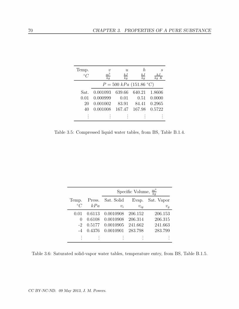
3.4.4.4 Compressed liquid water tables
Liquids truly have properties which vary with both T and P . To capture such variation,we can use compressed liquid tables as an equation of state. An example for water is givenin Table 3.5. If compressed liquid tables do not exist, it is usually safe enough to assumeproperties are those for x = 0 saturated liquid at the appropriate temperature.
3.4.4.5 Saturated water, solid-vapor
Other types of saturation can exist. For example, below the triple point temperature, onecan have solid water in equilibrium with water vapor. The process where ice transformsdirectly to water vapor is known as sublimation. Saturation tables for ice-vapor equilibriumexist as well. For example, consider the structure of saturation tables, as shown in Table3.6, extracted from BS’s Table B.1.5.
CC BY-NC-ND. 09 May 2013, J. M. Powers.
70 CHAPTER 3. PROPERTIES OF A PURE SUBSTANCE
Temp. v u h s◦C m3
kgkJkg
kJkg
kJkg K
P = 500 kPa (151.86 ◦C)
Sat. 0.001093 639.66 640.21 1.86060.01 0.000999 0.01 0.51 0.0000
20 0.001002 83.91 84.41 0.296540 0.001008 167.47 167.98 0.5722
......
......
...
Table 3.5: Compressed liquid water tables, from BS, Table B.1.4.
Specific Volume, m3
kg
Temp. Press. Sat. Solid Evap. Sat. Vapor◦C kPa vi vig vg
0.01 0.6113 0.0010908 206.152 206.1530 0.6108 0.0010908 206.314 206.315-2 0.5177 0.0010905 241.662 241.663-4 0.4376 0.0010901 283.798 283.799...
......
......
Table 3.6: Saturated solid-vapor water tables, temperature entry, from BS, Table B.1.5.
CC BY-NC-ND. 09 May 2013, J. M. Powers.

3.4. THERMAL EQUATIONS OF STATE 71
3.4.4.6 Tables for other materials
For many materials similar tables exist, e.g., ammonia, NH3. Consider the ammonia satura-tion tables, as shown in Table 3.7, extracted from BS’s Table B.2.1. One also has tables for
Specific Volume, m3
kg
Temp. Press. Sat. Liquid Evap. Sat. Vapor◦C kPa vf vfg vg
-50 40.9 0.001424 2.62557 2.62700-45 54.5 0.001437 2.00489 2.00632-40 71.7 0.001450 1.55111 1.55256-35 93.2 0.001463 1.21466 1.21613
......
......
...132.3 11333.2 0.004255 0 0.004255
Table 3.7: Saturated liquid-vapor ammonia tables, temperature entry, from BS, Table B.2.1.
superheated ammonia vapor. An example of a portion of such a table is shown in Table 3.8.Other tables in BS, include those for carbon dioxide, CO2, a modern refrigerant, R-410a,11
Temp. v u h s◦C m3
kgkJkg
kJkg
kJkg K
P = 50 kPa (−46.53 ◦C)
Sat. 2.1752 1269.6 1378.3 6.0839-30 2.3448 1296.2 1413.4 6.2333-20 2.4463 1312.3 1434.6 6.3187-10 2.5471 1328.4 1455.7 6.4006
......
......
...
Table 3.8: Superheated ammonia tables, from BS, Table B.2.2.
another common refrigerant, R-134a,12 diatomic nitrogen, N2, and methane, CH4.
3.4.4.7 Linear interpolation of tabular data
• interpolation is often required when exact values are not tabulated.
11a common cooling fluid invented in 1991, a near-azeotropic mixture of difluoromethane and pentafluo-roethane.
12a cooling fluid which became common in the 1990s, 1,1,1,2-tetrafluoroethane.
CC BY-NC-ND. 09 May 2013, J. M. Powers.

72 CHAPTER 3. PROPERTIES OF A PURE SUBSTANCE
• in this course we will primarily use linear interpolations.
• use extrapolations only if there is no other choice.
• occasionally double interpolations will be necessary.
3.4.4.7.1 Single interpolation The most common interpolation is the single interpo-lation of variables. We give an example here.
Example 3.5Given water at T = 36.7 ◦C, with v = 10 m3/kg, find the pressure and the quality if a two-phase
mixture.
A wise first step is to go to the saturated tables. We check Table B.1.1 from BS and find there areno values at T = 36.7 ◦C. So we must create our own personal steam table values at this temperature,just to determine if where we are on the thermodynamic surface. We list the important part of thesaturated water liquid-vapor tables in Table 3.9.
Specific Volume, m3
kg
Temp. Press. Sat. Liquid Evap. Sat. Vapor◦C kPa vf vfg vg
......
......
...35 5.628 0.001006 25.2148 25.2158
36.7 ? ? ? ?40 7.384 0.001008 19.5219 19.5229
......
......
...
Table 3.9: Relevant portion of saturated liquid-vapor water tables, temperature entry, fromBS, Table B.1.1.
We seek to get appropriate values for P , vf , vfg, and vg at T = 36.7 ◦C. Let us find P first. Theessence of linear interpolation is to fit known data to a straight line, then use the formula of that line topredict intermediate values of variables of interest. We know values of P at T = 35 ◦C and T = 40 ◦C.In fact we have two points: (T1, P1) = (35 ◦C, 5.628 kPa), and (T2, P2) = (40 ◦C, 7.384 kPa). This letsus fit a line using the familiar point-slope formula:
P − P1 =
(P2 − P1
T2 − T1
)
︸ ︷︷ ︸
slope
(T − T1). (3.69)
We could have used the other point. Note when T = T1, that P = P1. Also, when T = T2, P = P2.
CC BY-NC-ND. 09 May 2013, J. M. Powers.
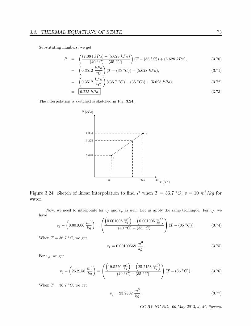
3.4. THERMAL EQUATIONS OF STATE 73
Substituting numbers, we get
P =
((7.384 kPa) − (5.628 kPa)
(40 ◦C) − (35 ◦C)
)
(T − (35 ◦C)) + (5.628 kPa), (3.70)
=
(
0.3512kPa◦C
)
(T − (35 ◦C)) + (5.628 kPa), (3.71)
=
(
0.3512kPa◦C
)
((36.7 ◦C) − (35 ◦C)) + (5.628 kPa), (3.72)
= 6.225 kPa. (3.73)
The interpolation is sketched is sketched in Fig. 3.24.
T (oC )
P (kPa)
35 36.7 40
7.384
6.225
5.6281
2
Figure 3.24: Sketch of linear interpolation to find P when T = 36.7 ◦C, v = 10 m3/kg forwater.
Now, we need to interpolate for vf and vg as well. Let us apply the same technique. For vf , wehave
vf −(
0.001006m3
kg
)
=
(
0.001008 m3
kg
)
−(
0.001006 m3
kg
)
(40 ◦C) − (35 ◦C)
(T − (35 ◦C)). (3.74)
When T = 36.7 ◦C, we get
vf = 0.00100668m3
kg. (3.75)
For vg, we get
vg −(
25.2158m3
kg
)
=
(
19.5229 m3
kg
)
−(
25.2158 m3
kg
)
(40 ◦C) − (35 ◦C)
(T − (35 ◦C)). (3.76)
When T = 36.7 ◦C, we get
vg = 23.2802m3
kg. (3.77)
CC BY-NC-ND. 09 May 2013, J. M. Powers.

74 CHAPTER 3. PROPERTIES OF A PURE SUBSTANCE
Knowing vf and vg, we do not need to interpolate for vfg. We can simply use the definition:
vfg = vg − vf =
(
23.2802m3
kg
)
−(
0.00100668m3
kg
)
= 23.2792m3
kg. (3.78)
Now, v = 10 m3/kg. Since at T = 36.7◦C, we have vf < v < vg, we have a two-phase mixture.Let us get the quality. From Eq. (3.61), we have
x =v − vf
vfg=
(
10 m3
kg
)
−(
0.00100668 m3
kg
)
23.2792 m3
kg
= 0.429525. (3.79)
Thus
x =mvap
mtot= 0.429525. (3.80)
3.4.4.7.2 Double interpolation Sometimes, we need to do extra linear interpolations.Say we are given superheated water with vo and To and we are asked to find Po. But neithervo nor To are listed in the tables. Then we need to do a multi-step procedure.
• Go to the tables and for the given To and vo, estimate approximately the value of Po
by visual examination.
• For a nearby value of P = P1, get a linear interpolation of the form T = T (v, P1). Usethis to get T1 = T (vo, P1).
• For a different nearby value of P = P2, get another linear interpolation of the formT = T (v, P2). Use this to get T2 = T (vo, P2). We now have two points (T1, P1) and(T2, P2), both valid at v = vo.
• Use the two points (T1, P1), (T2, P2) to develop a third interpolation P = P (T, vo).Estimate Po by Po = P (To, vo).
Example 3.6Consider m = 1 kg of H2O initially at T1 = 110 ◦C, x1 = 0.9. The H2O is heated until T2 = 200 ◦C.
As sketched in Fig. 3.25, the H2O is confined in a piston-cylinder arrangement, where the pistonis constrained by a linear spring with dP/dv = 40 kPa/m3/kg. At the initial state, the spring isunstretched. Find the final pressure.
While this problem seems straightforward, there are many challenges. Let us first consider whatwe know about the initial state. Since we have a numerical value for x1, we know state 1 is a two-phasemixture. From the tables, we find that
P1 = 143.3 kPa, vf1 = 0.001052m3
kg, vg1 = 1.2101
m3
kg, vfg1 = 1.20909
m3
kg. (3.81)
CC BY-NC-ND. 09 May 2013, J. M. Powers.

3.4. THERMAL EQUATIONS OF STATE 75
PA
PatmAFs=k(y-y1)
water
free body diagram
Figure 3.25: Sketch of piston-cylinder arrangement.
We can then calculate v1 for the mixture:
v1 = vf1 + x1vfg1 =
(
0.001052m3
kg
)
+ (0.9)
(
1.20909m3
kg
)
= 1.08923m3
kg. (3.82)
We now know everything we need about state 1.At state 2, we only know one intensive thermodynamic property, the temperature, T2 = 200 ◦C.
• To get a second, and thus define the final state, we will need to bring in information about the process.
Now, we will need to consider a force balance on the piston. Newton’s second law for the piston says
mpistond2y
dt2=∑
Fy. (3.83)
From our free body diagram, we note three major forces:
• force due to the interior pressure from the water,
• force due to the exterior pressure from the atmosphere,
• force due to the linear spring, which we call Fs = k(y − y1) where k is the spring constant, y is theposition of the piston, and y1 is the initial position of the piston. Note that Fs = 0 when y = y1.
We write this as
mpistond2y
dt2= PA − PatmA − k(y − y1). (3.84)
Now, in classical thermodynamics, we make the assumption that the inertia of the piston is so smallthat we can neglect its effect. We are really requiring that a force balance exist for all time. Thus,even though the piston will move, and perhaps accelerate, its acceleration will be so small that it canbe neglected relative to the forces in play. We thus take
∣∣∣∣mpiston
d2y
dt2
∣∣∣∣≪ |Fs|, |PatmA|, |PA|. (3.85)
With this assumption, we have
0 ≃ PA − PatmA − k(y − y1). (3.86)
Solve for P , the water pressure, to get
P = Patm +k
A(y − y1). (3.87)
CC BY-NC-ND. 09 May 2013, J. M. Powers.

76 CHAPTER 3. PROPERTIES OF A PURE SUBSTANCE
Now, V = Ay and V1 = Ay1, so we can say
P = Patm +k
A2(V − V1). (3.88)
Let us use the fact that V = mv and V1 = mv1 to rewrite as
P = Patm +km
A2(v − v1). (3.89)
This equation is highlighted because it provides an algebraic relationship between two intensive thermo-
dynamic properties, P and v, and such a tactic will be useful for many future problems. Using numbersfrom our problem, with dP/dv = km/A2, we can say
P = (143.3 kPa) +
(
40kPam3
kg
)(
v −(
1.08923m3
kg
))
, (3.90)
P = (99.7308 kPa) +
(
40kPam3
kg
)
v.
︸ ︷︷ ︸
linear spring rule
(3.91)
Now, at state 1, we have V = V1 and P = P1 = 143.3 kPa, so we must have Patm = 143.3 kPa for thisproblem.
Let us now consider the possibilities for state 2. We are constrained to be on the line in P −v spacegiven by our force balance, Eq. (3.91). We are also constrained to be on the T = 200 ◦C isotherm,which is also a curve in P − v space. So let us consider the P − v plane, as sketched in Fig. 3.26. The
v
P
T1=110 oC
T2=200 oC
v
P
T1 =110 oC
T2 =200 oC
km/A2 ~ large
km/A2 ~ small
1
2
1
2
Figure 3.26: Sketch of P − v plane for piston-cylinder-linear spring problem for water.
isotherms for T1 = 110 ◦C and T2 = 200 ◦C are set in both parts of Fig. 3.26. Since both T1 and T2 arewell below Tc, both isotherms pierce the vapor dome. Our final state has a line in P − v space from theforce balance intersecting the state 2 isotherm. There are two distinct possibilities for the final state:
• for a stiff spring, i.e. large km/A2, our line will intersect the isotherm within the vapor dome, or
• for a loose spring, i.e. small km/A2, our line will intersect the isotherm in the superheated vaporregion.
Let us consider the first possibility: state 2 is under the vapor dome. If that is the case, then thetables tell us that P2 = 1553.8 kPa. At this pressure, Eq. (3.91) gives us v = (1553.8− 99.7308)/40 =
CC BY-NC-ND. 09 May 2013, J. M. Powers.
3.4. THERMAL EQUATIONS OF STATE 77
36.3517 m3/kg. However, at this pressure vg = 0.12736 m3/kg. Since we just found v > vg, ourassumption that the final state was under the dome must be incorrect!
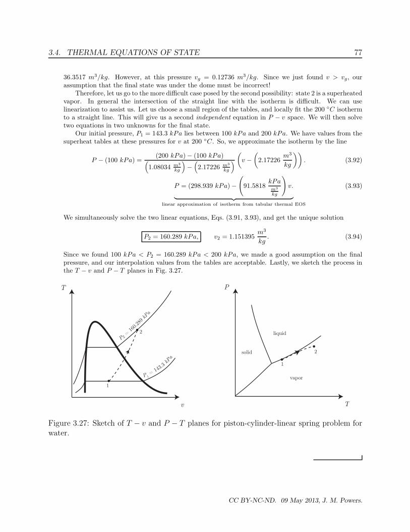
Therefore, let us go to the more difficult case posed by the second possibility: state 2 is a superheatedvapor. In general the intersection of the straight line with the isotherm is difficult. We can uselinearization to assist us. Let us choose a small region of the tables, and locally fit the 200 ◦C isothermto a straight line. This will give us a second independent equation in P − v space. We will then solvetwo equations in two unknowns for the final state.
Our initial pressure, P1 = 143.3 kPa lies between 100 kPa and 200 kPa. We have values from thesuperheat tables at these pressures for v at 200 ◦C. So, we approximate the isotherm by the line
P − (100 kPa) =(200 kPa) − (100 kPa)
(
1.08034 m3
kg
)
−(
2.17226 m3
kg
)
(
v −(
2.17226m3
kg
))
. (3.92)
P = (298.939 kPa) −(
91.5818kPam3
kg
)
v.
︸ ︷︷ ︸
linear approximation of isotherm from tabular thermal EOS
(3.93)
We simultaneously solve the two linear equations, Eqs. (3.91, 3.93), and get the unique solution
P2 = 160.289 kPa, v2 = 1.151395m3
kg. (3.94)
Since we found 100 kPa < P2 = 160.289 kPa < 200 kPa, we made a good assumption on the finalpressure, and our interpolation values from the tables are acceptable. Lastly, we sketch the process inthe T − v and P − T planes in Fig. 3.27.
v
T
T
P
1
2
1
2
P2 = 1
60.289
k
Pa
liquid
solid
vaporP 1 = 14
3.3 k
Pa
Figure 3.27: Sketch of T − v and P − T planes for piston-cylinder-linear spring problem forwater.
CC BY-NC-ND. 09 May 2013, J. M. Powers.

78 CHAPTER 3. PROPERTIES OF A PURE SUBSTANCE
CC BY-NC-ND. 09 May 2013, J. M. Powers.