Physics 235 Chapter 3

- 1 -

Chapter 3 Oscillations

In this Chapter different types of oscillations will be discussed. A particle carrying out oscillatory motion, oscillates around a stable equilibrium position (note: if the equilibrium position was a position of unstable equilibrium, the particle would not return to its equilibrium position, and no oscillatory motion would result). We will not only focus on harmonic motion in one dimension but also consider motion in two- or three-dimensions. In addition, we will discuss damped motion and driven motion. Simple-Harmonic Motion in One Dimension Since we have the freedom to choose the origin of our coordinate system, we can choose it to coincide with the equilibrium position of our oscillator. The force that is responsible for the harmonic motion can be expanded around the equilibrium position:

where F0 is the force at x = 0. Since x = 0 is the equilibrium point, the force at this point must be 0. If the displacement x is small, we can ignore all terms involving x2 and higher powers. The force can thus be approximated by

Note: the constant k is positive since dF/dx must be negative if the equilibrium point is a point of stable equilibrium. A force that is proportional to –kx is said to obey Hooke’s law. Since the force F is equal to ma, we can rewrite the previous equation as

This equation is frequently rewritten as

where w0 is the angular frequency of the harmonic motion. The most general solution of this differential equation is A sin(w0t - f). The amplitude and the phase angle must be determined to match the initial conditions (for example, the position and velocity at time t = 0 may have been

F x( ) = F0 + xdFdx

⎛⎝⎜

⎞⎠⎟ 0

+ x2

2!d 2Fdx2

⎛⎝⎜

⎞⎠⎟ 0

+ x3

3!d 3Fdx3

⎛⎝⎜

⎞⎠⎟ 0

+ ....

F x( ) = x dFdx

⎛⎝⎜

⎞⎠⎟ 0

= −kx

!!x + kmx = 0

!!x +ω 02x = 0

Physics 235 Chapter 3

- 2 -

specified). The total energy of the harmonic oscillator is constant, but the kinetic and potential energy components of the total energy are time dependent. The angular frequency of the harmonic motion is independent of the amplitude of the motion. Systems that have this property are called isochronous systems. Note: keep in mind though that only for small oscillations the force might be proportional to the displacement. This means that only for small displacements, the motion will be simple harmonic; for larger displacements the angular frequency may become dependent on amplitude. Simple-Harmonic Motion in Two Dimensions When we discuss simple-harmonic motion in two dimensions we can always decompose the motion into two components, each directed along one of the two coordinate axes. We need to consider two special cases: • The motion is a result of a single force, which obeys Hooke’s law. The force can be

written as:

Of course, one can argue that with the proper choice of coordinate system, this can be considered one-dimensional motion. However, the reason that the solution discussed in the previous section is not the general solution in the two-dimensional case is due to the fact that the initial conditions, such as the velocity at time t = 0, does not have to be directed in the same direction as the position vector r. If we decompose the position vector r into its components along the x and y axes, we get the following differential equations that must be satisfied by the oscillator:

The resulting motion will be thus the combined motion of two simple-harmonics oscillators, one along each axes, with the same angular frequency but different amplitudes and phase angles:

Although these equations of motion are simple, the easiest way to examine this type of motion is by actually looking at plots of for example, the trajectory carried out by the particle. You can use

F!"

F = −kr

!!x +ω 02x = 0

!!y +ω 02y = 0

x t( ) = Acos(ω 0t −α )

y t( ) = Bcos(ω 0t − β )

Physics 235 Chapter 3

- 3 -

the Excel document SHM2DOneF.xls to study the motion of this two-dimensional oscillator. Examples of trajectories for A = B = 1 m, a = 180°, b = 0° and A = B = 1 m, a = 90°, b = 45° are shown in Figure 1.

Figure 1. Two-dimensional motion of a simple-harmonic oscillator with A = B = 1 m, a = 180°, b = 0° (left) and A = B = 1 m, a = 90°, b = 45° (right). The angular frequencies of the motion in the x and y directions are taken to be the same.

Since the angular frequency of the motion in the x direction is the same as the angular frequency of the motion in the y direction, the trajectory of the particle will be a closed trajectory (that is, after a given period T, the particle will return to the same position and have the same velocity and acceleration; the motion is truly periodic).

• The motion is a result of a several forces, which each obey Hooke’s law. Now consider what happens if we have several forces acting on the particle. Since each of these forces may have a different force constant, the angular frequency of the motion along the x axis may be different from the angular frequency of the motion along the y axis:

The corresponding x and y positions as function of time are

!!x +ω A2x = 0

!!y +ω B2y = 0

x t( ) = Acos(ω At −α )

y t( ) = Bsin(ω Bt − β )

Physics 235 Chapter 3

- 4 -

The biggest difference between this case of multiple forces and the previously discussed case of a single force is that in the former case there is no guarantee that the trajectory is closed (except when wA/wB is a rational fraction), while in the latter case every trajectory is closed, independent of the initial conditions. The trajectory described by the particle is called a Lissajous curve. Examples of such curves for two slightly different sets of parameters are shown in Figure 2 for A = B = 1 m, a = 0°, b = 135°, wA = 1 rad/s, wB = 2 rad/s (left) and A = B = 1 m, a = 0°, b = 135°, wA = 1 rad/s, wB = 2.1 rad/s (right). You can use the Excel document SHM2DTwoF.xls to study the motion of this two-dimensional oscillator in more detail.

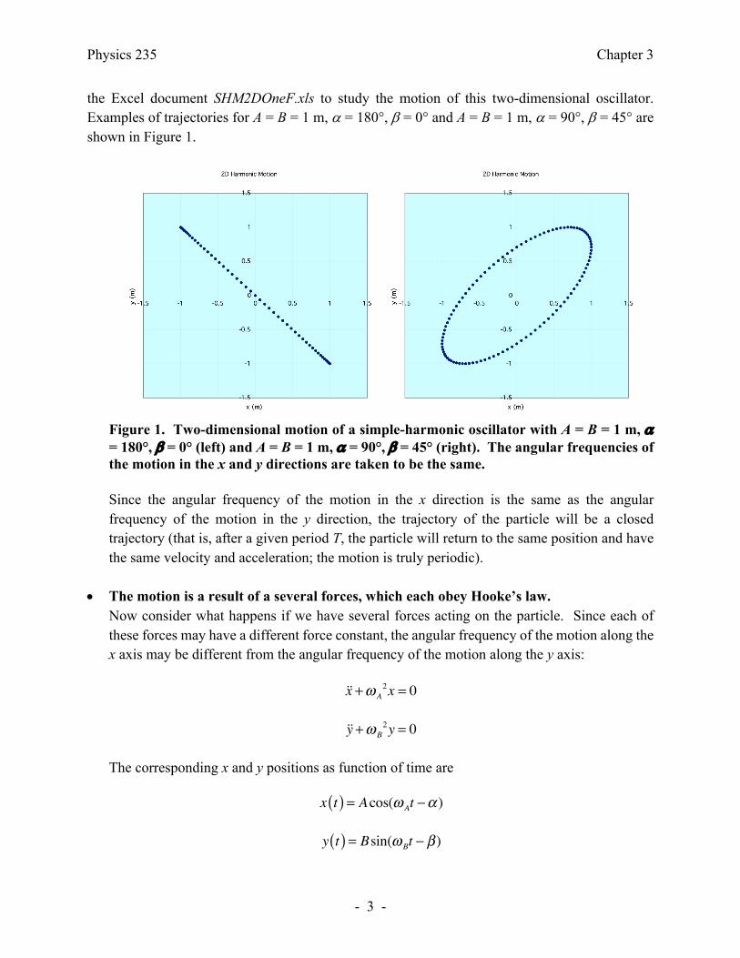
Figure 2. Lissajous curve for A = B = 1 m, a = 0°, b = 135°, wA = 1 rad/s, wB = 2 rad/s (left) and A = B = 1 m, a = 0°, b = 135°, wA = 1 rad/s, wB = 2.1 rad/s (right). Phase Diagrams Although the trajectory of the particle in real space is one way to visualize the information of the motion of the oscillators, in general it does not provide information about important parameters such as the total energy of the system. More detailed information is provided by phase diagrams; they show simultaneous information about the position and the velocity of the particle (which is the information that is required to uniquely specify the motion of the simple-harmonic oscillator). For example, a phase diagram for a one-dimensional oscillator is a two-dimensional figure showing velocity versus position. Figure 3 shows a phase diagram for a one-dimensional simple-harmonic oscillator; it shows three phase paths, corresponding to three different total energies. A few important observations about phase diagrams can be made: • Two phase paths can not cross. If they would cross at a particular point, then the total energy

at that point would not be defined (it would have two possible values).

Physics 235 Chapter 3

- 5 -

• The phase paths will be executed in a clock-wise direction. For example, in the upper right corner of the phase diagram, the velocity is positive. This implies that x must be increasing. The x coordinate will continue to increase until the velocity becomes equal to zero.

Figure 3. Phase diagram for a one-dimensional simple-harmonic oscillator

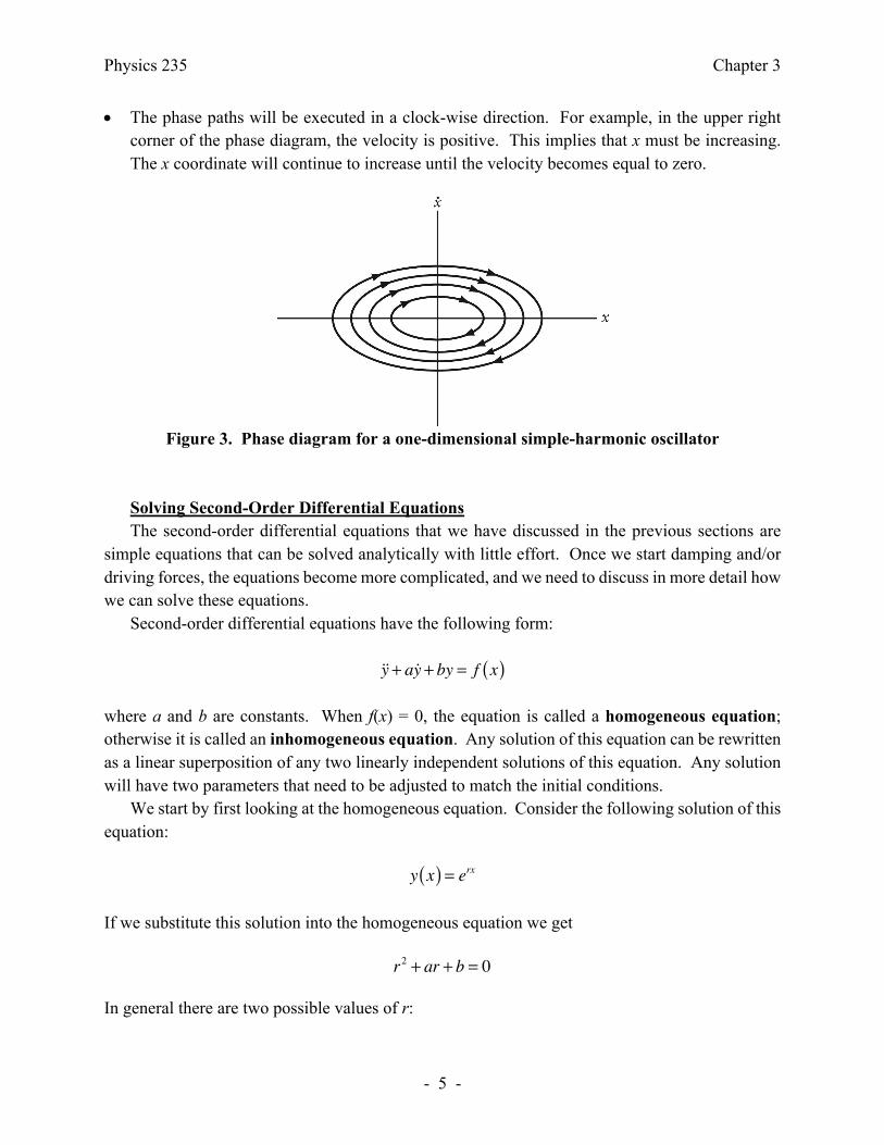
Solving Second-Order Differential Equations The second-order differential equations that we have discussed in the previous sections are simple equations that can be solved analytically with little effort. Once we start damping and/or driving forces, the equations become more complicated, and we need to discuss in more detail how we can solve these equations. Second-order differential equations have the following form:

where a and b are constants. When f(x) = 0, the equation is called a homogeneous equation; otherwise it is called an inhomogeneous equation. Any solution of this equation can be rewritten as a linear superposition of any two linearly independent solutions of this equation. Any solution will have two parameters that need to be adjusted to match the initial conditions. We start by first looking at the homogeneous equation. Consider the following solution of this equation:

If we substitute this solution into the homogeneous equation we get

In general there are two possible values of r:

!!y + a!y + by = f x( )

y x( ) = erx

r2 + ar + b = 0

Physics 235 Chapter 3

- 6 -

If a2 ≠ 4b then we can write the general solution to the homogeneous differential equation as

This is the most general solution to the homogeneous differential equation since its two terms are linearly independent. If a2 = 4b then there is only one solution for r and there must be another solution of the differential equation. Consider the function xerx, where r = -a/2. This is a solution of the homogeneous differential equation, which we can verify by substituting it into the equation:

Since the functions xerx and erx are linearly independent, the most general solution can be written as

If a2 < 4b, the solutions for r are complex numbers:

and the general solution can be rewritten as

Now we continue and consider the inhomogeneous equation

Consider that u is the general solution of the corresponding homogenous solution (u is called the complementary function) and v is a solution of the inhomogeneous equation (v is called the a particular solution). This requires that

and

r± = − a2± 12

a2 − 4b

y x( ) = c1e−a2+12

a2−4b⎛⎝⎜

⎞⎠⎟ x + c2e

−a2−12

a2−4b⎛⎝⎜

⎞⎠⎟ x

d 2

dx2xerx( )+ a ddx xerx( )+ b xerx( ) = 2r + a( )erx + r2 + ar + b( )xerx = 0

y x( ) = c1e−a2

⎛⎝⎜

⎞⎠⎟ x + c2xe

−a2

⎛⎝⎜

⎞⎠⎟ x

r± =α ± iβ

y x( ) = eαx c1 cosβx + c2 sinβx( )

!!y + a!y + by = f x( )

!!u + a !u + bu = 0

Physics 235 Chapter 3

- 7 -

The function u + v is now also a solution of the inhomogeneous solution, and since it contains two constants (since u is the general solution of the homogeneous solution), it must be the general solution of the inhomogeneous equation. Damped Oscillations A damped oscillator has a restoring force that satisfies Hooke’s law and a damping force that may be a function of velocity. The differential equation that describes the damped motion is

or

where b is the damping parameter. The general solution of the differential equation, which can be solved analytically, is

The corresponding velocity is equal to

There are three distinct modes of oscillations described by this general solution. We illustrate these modes by focusing on three distinct cases of damping. In each case, we assume that at time t = 0, the displacement is x0 and the velocity it v0. The phase diagrams for these examples can be explored using the Excel document DampedMotion.xls. • Critical Damping: w02 = b2.

In this case the position and velocity are given by

and

!!v + a !v + bv = f x( )

m!!x + b !x + kx = 0

!!x + bm!x + k

mx = !!x + 2β !x +ω 0

2x = 0

x t( ) = e−βt A1eβ 2−ω0

2 t + A2e− β 2−ω0

2 t{ }

v t( ) = β 2 −ω 02 − β{ }A1e−βte β 2−ω0

2 t − β 2 −ω 02 + β{ }A2e−βte− β 2−ω0

2 t

x t( ) = A1e−βt + A2te−βt

Physics 235 Chapter 3

- 8 -

In order to satisfy the boundary conditions we must require that

or

An example of a phase diagram for critical damping is shown in Figure 4 (left).

Figure 4. Phase diagram of critically damped harmonic motion with w0 = 1 rad/s and b = 1 Ns/m (left) and over damped harmonic motion with w0 = 1 rad/s, and b = 2 Ns/m (right).

• Over damping: w02 < b 2.

In this case, the position and velocity are given by

and

v t( ) = −βA1e−βt + A2 e

−βt − βte−βt( )

x 0( ) = A1 = x0

v 0( ) = −βA1 + A2 = −βx0 + A2 = v0

A1 = x0

A2 = v0 + βx0

x t( ) = e−βt A1eβ 2−ω0

2 t + A2e− β 2−ω0

2 t{ }

Physics 235 Chapter 3

- 9 -

To match the boundary conditions we must require that

or

An example of a phase diagram for over damping is shown in Figure 4 (right).

• Under damping: w02 > b 2. In this case, the position and velocity are given by

and

To satisfy the boundary conditions we must require that

or

v t( ) = e−βt A1 β 2 −ω 02 − β{ }e β 2−ω0

2 t − A2 β 2 −ω 02 + β{ }e− β 2−ω0

2 t{ }

x 0( ) = A1 + A2 = x0

v 0( ) = A1 β 2 −ω 02 − β{ }− A2 β 2 −ω 0

2 + β{ } = v0

A1 =x0 β 2 −ω 0

2 + β{ }+ v02 β 2 −ω 0

2

A2 =x0 β 2 −ω 0

2 − β{ }− v02 β 2 −ω 0

2

x t( ) = e−βt A1 cos ω 02 − β 2 t( )+ A2 sin ω 0

2 − β 2 t( ){ }

v t( ) = e−βt −βA1 + ω 02 − β 2A2( )cos ω 0

2 − β 2 t( )− βA2 + ω 02 − β 2( )sin ω 0

2 − β 2 t( ){ }

x 0( ) = A1 = x0

v 0( ) = −βA1 + ω 02 − β 2A2 = v0

A1 = x0

Physics 235 Chapter 3

- 10 -

Examples of phase diagrams for under damping are shown in Figure 5.

Figure 5. Phase diagram of under damped harmonic motion with w0 = 1 rad/s, and b = 0.5 Ns/m (left) and w0 = 1 rad/s, and b = 0.1 Ns/m (right).

A comparison of the displacement as function of time for the three types of damping is shown in Figure 6. For a given set of initial conditions (same displacement and velocity) we see that the critically damped oscillator approaches the equilibrium position at a rate that is higher than either the under damped or the over damped oscillator.

Figure 6. Displacement as function of time for a one-dimensional damped oscillator.

A2 =βA1 + v0ω 0

2 − β 2

Physics 235 Chapter 3

- 11 -

Driven Motion We will start out discussion of driven motion by considering an external driving force that varies in a harmonic fashion as function of time. The equation of motion for an oscillator exposed to the driving force is given by

The general solution for the complementary solution has already been discussed previously and is given by

A particular solution is

where

This can be verified by substituting this solution in the original differential equation.

!!x + 2β !x +ω 02x = Acos ωt( )

xc t( ) = e−βt A1eβ 2−ω0

2 t + A2e− β 2−ω0

2 t{ }

xp t( ) = A

ω 02 −ω 2( )2 + 4ω 2β 2

cos ωt −δ( )

δ = tan−1 2ωβω 0

2 −ω 2

⎛⎝⎜

⎞⎠⎟

Figure 7. Examples of sinusoidal driven oscillatory motion with damping.

Physics 235 Chapter 3

- 12 -

The complementary solution has an amplitude which decreases exponentially as function of time, while the amplitude of the particular solution is independent of time. As a result, for long times, the motion will be dominated by the particular solution, and this solution represents the steady-state solution. The transient effects may be dominated by the complementary solution. Figure 7 shows examples of complementary functions and particular solutions for a driven oscillator with damping. The amplitude of the steady-state solution of the driven harmonic oscillator is a function of the angular frequency w of the driving force and the “natural” angular frequency of the oscillator. There are three different resonance frequencies for the system: • The amplitude resonance frequency. This is the frequency for which the amplitude has a

maximum. This requires that

or

The amplitude has a maximum when the driving frequency is equal to

• The kinetic energy resonance frequency. The kinetic energy of the oscillator, in its steady-

state condition, is equal to

The average kinetic energy, averaged over one period, is equal to

The average kinetic energy has a maximum when

ddω

A

ω 02 −ω 2( )2 + 4ω 2β 2

⎛

⎝

⎜⎜

⎞

⎠

⎟⎟= −

−2ω ω 02 −ω 2( )+ 4ωβ 2

ω 02 −ω 2( )2 + 4ω 2β 2( )3/2

A = 0

ω −ω 02 +ω 2 + 2β 2( ) = 0

ω R = ω 02 − 2β 2

T = 12m!x2 = 1

2m −Aω

ω 02 −ω 2( )2 + 4ω 2β 2

sin ωt −δ( )⎛

⎝

⎜⎜

⎞

⎠

⎟⎟

2

= 12m A2ω 2

ω 02 −ω 2( )2 + 4ω 2β 2

sin2 ωt −δ( )

T = 12m A2ω 2

ω 02 −ω 2( )2 + 4ω 2β 2

sin2 ωt −δ( ) = 14m A2ω 2

ω 02 −ω 2( )2 + 4ω 2β 2

Physics 235 Chapter 3

- 13 -

This happens when the driving frequency w equal to natural frequency w0.

• The potential energy resonance frequency. Since the potential energy is proportional the displacement squared, the potential energy will have a maximum when the displacement has a maximum. This resonance frequency will thus be the same as the amplitude resonance frequency. Although in general the driving force will not be a simple harmonic function, the discussion in

this Section is useful since any arbitrary function can be expanded in a series of harmonic functions. Consider a driving force F(t) and assume the driving force has a period t. Consider that the force F can be expanded in the following way in terms of simple harmonic functions:

where

Consider the following integrals:

They can be used to express determine the coefficients an and bn:

d Tdω

= 14m 2A2ω

ω 02 −ω 2( )2 + 4ω 2β 2

−A2ω 2 8ωβ 2 − 4ω ω 0

2 −ω 2( )( )ω 0

2 −ω 2( )2 + 4ω 2β 2( )2⎧

⎨⎪

⎩⎪

⎫

⎬⎪

⎭⎪=

= 14m

2A2ω 2 ω 02 −ω 2( ) ω 0

2 +ω 2( )ω 0

2 −ω 2( )2 + 4ω 2β 2( )2⎧

⎨⎪

⎩⎪

⎫

⎬⎪

⎭⎪

F t( ) = 12a0 + an cosnωt + bn sinnωt( )

n=1

∞

∑

ω = 2πτ

F t '( )cos nωt '( )0

τ

∫ dt ' = F t '( )cos nωt '( )0

τ

∫ dt ' = an cos2 nωt '( )dt '

0

τ

∫ = annϖ

cos2 x( )dx0

nωτ

∫ = anτ2

F t '( )sin nωt '( )0

τ

∫ dt ' = F t '( )sin nωt '( )0

τ

∫ dt ' = bn sin2 nωt '( )dt '

0

τ

∫ = bnnϖ

sin2 x( )dx0

nωτ

∫ = bnτ2

Physics 235 Chapter 3

- 14 -

When we apply the for F(t) to the oscillator, we need to solve the following differential equation to determine the motion of the oscillator:

In order to solve this equation, we rely on the principle of superposition. Consider the function x1 and x2 which satisfy the following differential equations:

Adding these two equations we obtain the following relation:

We thus see that (x1 + x2) is a solution of the differential equation with a driving force of (F1 + F2). We can thus solve the differential equation for the driving force F(t) if we solve each of the following differential equations:

The solution to the first equation is

where

an =2τ

F t '( )cos nωt '( )dt '0

τ

∫

bn =2τ

F t '( )sin nωt '( )dt '0

τ

∫

!!x + 2β !x +ω 02x = 1

2a0 + an cosnωt + bn sinnωt( )

n=1

∞

∑

!!x1 + 2β !x1 +ω 02x1 = F1

!!x2 + 2β !x2 +ω 02x2 = F2

!!x1 + !!x2( )+ 2β !x1 + !x2( )+ω 02 x1 + x2( ) = F1 + F2

!!x + 2β !x +ω 02x = cosnωt = cosω nt

!!x + 2β !x +ω 02x = sinnωt = sinω nt

!!x + 2β !x +ω 02x = 1

2

x t( ) = A

ω 02 −ω n

2( )2 + 4ω n2β 2

cos ω nt −δ n( )

Physics 235 Chapter 3

- 15 -

The solution of the second equation is

where

The solution to the third equation is

The solution of the following differential equation

is thus equal to

where

and

δ n = tan−1 2ω nβ

ω 02 −ω n

2

⎛⎝⎜

⎞⎠⎟

x t( ) = B

ω 02 −ω n

2( )2 + 4ω n2β 2

sin ω nt −δ n( )

δ n = tan−1 2ω nβ

ω 02 −ω n

2

⎛⎝⎜

⎞⎠⎟

x = 12ω 0

2

!!x + 2β !x +ω 02x = 1

2a0 + an cosnωt + bn sinnωt( )

n=1

∞

∑

x t( ) = a02ω 0

2 +1

ω 02 −ω n

2( )2 + 4ω n2β 2

an cos ω nt −δ n( )+ bn sin ω nt −δ n( )( )n=1

∞

∑

δ n = tan−1 2ω nβ

ω 02 −ω n

2

⎛⎝⎜

⎞⎠⎟

ω n = nω

Physics 235 Chapter 3

- 16 -

Updated on 9/1/19 7:26 PM.