Chapter 3 Hyperbolic Position Location Systems location... · 2006-02-01 · CHAPTER 3. HYPERBOLIC...

Chapter 3

Hyperbolic Position Location

Systems

3.1 Introduction

This chapter introduces the general models for the position location problem and the

techniques involved in the hyperbolic position location method. Hyperbolic position

location (PL) estimation is accomplished in two stages. The first stage involves

estimation of the time difference of arrival (TDOA) between receivers through the use

of time delay estimation techniques. The estimated TDOA’s are then transformed into

range difference measurements between base stations, resulting in a set of nonlinear

hyperbolic range difference equations. The second stage utilizes efficient algorithms

to produce an unambiguous solution to these nonlinear hyperbolic equations. The

solution produced by these algorithms result in the estimated position location of

the source. The following sections introduce the techniques and algorithms used to

perform hyperbolic position location of a mobile user.

34

CHAPTER 3. HYPERBOLIC POSITION LOCATION SYSTEMS 35

3.2 TDOA Estimation Techniques

The time difference of arrival (TDOA) of a signal can be estimated by two general

methods: subtracting TOA measurements from two base stations to produce a relative

TDOA, or through the use of cross-correlation techniques, in which the received signal

at one base station is correlated with the received signal at another base station. The

former method requires knowledge of the transmit timing, and thus, strict clock

synchronization between the base stations and source. To eliminate the need for

knowledge of the source transmit timing, differencing of arrival times at the receivers is

commonly employed. Differencing the observed time of arrival eliminates some of the

errors in TOA estimates common to all receivers and reduces other errors because of

spatial and temporal coherence. While determining the TDOA from TOA estimates is

a feasible method, cross-correlation techniques dominate the field of TDOA estimation

techniques. As such, the discussion of TDOA estimation is limited to cross-correlation

estimation techniques. In the following section, a general model for TDOA estimation

is developed and the techniques for TDOA estimation are presented.

3.2.1 General Model for TDOA Estimation

For a signal, s(t), radiating from a remote source through a channel with interference

and noise, the general model for the time-delay estimation between received signals

at two base stations, x1(t) and x2(t), is given by

x1(t) = A1s(t− d1) + n1(t) (3.1)

x2(t) = A2s(t− d2) + n2(t),

where A1 and A2 are the amplitude scaling of the signal, n1(t) and n2(t) consist of

noise and interfering signals and d1 and d2 are the signal delay times, or arrival times.

This model assumes that s(t) , n1(t) and n2(t) are real and jointly stationary, zero-

mean (time average) random processes and that s(t) is uncorrelated with noise n1(t)

and n2(t). Referring the delay time and scaling amplitudes to the receiver with the

shortest time of arrival, assuming d1 < d2, the model of (3.1) can be rewritten as

x1(t) = s(t) + n1(t) (3.2)

x2(t) = As(t−D) + n2(t),


where A is the amplitude ratio and D = d2 − d1. It is desired to estimate D, the

time difference of arrival (TDOA) of s(t) between the two receivers. It may also be

desirable to estimate the scaling amplitude A. By estimating the amplitude scaling,

selection of the appropriate receivers can be made. It follows that the limit cyclic

cross-correlation and autocorrelations are given by

Rαx2x1

(τ ) = ARαs (τ −D)e−jπαD +Rα

n2n1(τ ) (3.3)

Rαx1

(τ ) = Rαs (τ ) +Rα

n1(τ ) (3.4)

Rαx2

(τ ) = |A|2Rαs (τ )e−jπαD +Rα

n2(τ ), (3.5)

where the parameter α is called the cycle frequency [Gar92a]. If α = 0, the above

equations are the conventional limit cross-correlation and autocorrelations.

If s(t) exhibits a cycle frequency α not shared by n1(t) and n2(t), then by using

this values of α in the measurements in (3.3)-(3.5), we obtain through infinite time

averaging

Rαn1

(τ ) = Rαn2

(τ ) = Rαn2n1

(τ ) = 0 (3.6)

and the general model for time delay estimation between base stations is

Rαx2x1

(τ ) = ARαs (τ −D)e−jπαD (3.7)

Rαx1

(τ ) = Rαs (τ ) (3.8)

Rαx2

(τ ) = |A|2Rαs (τ )e−jπαD. (3.9)

Accurate TDOA estimation requires the use of time delay estimation techniques that

provide resistance to noise and interference and the ability to resolve multipath sig-

nal components. Many techniques have been developed that estimate TDOA D

with varying degrees of accuracy and robustness. These include the generalized

cross-correlation (GCC) and cyclostationarity-exploiting cross-correlation methods.

Cyclostationarity-exploiting methods include the Cyclic Cross-Correlation (CYC-

COR), the Spectral-Coherence Alignment (SPECCOA) method, the Band-Limited

Spectral Correlation Ratio (BL-SPECCORR) method and the Cyclic Prony method

[Gar94]. While signal selective cyclostationarity-exploiting methods have been shown

in [Gar94] and [Gar92b] to outperform GCC methods in the presence of noise and in-

terference, they do so only when spectrally overlapping noise and interference exhibit

a cycle frequency different than the signal of interest. When spectrally overlapping


signals exhibit the same cycle frequency, as is encountered in multiuser CDMA sys-

tems, these methods do not offer an advantage over GCC methods. As such, only

generalized cross-correlation methods for TDOA estimation are presented.

3.2.2 Generalized Cross-Correlation Methods

Conventional correlation techniques that have been used to solve the problem of

TDOA estimation are referred to as generalized cross-correlation (GCC) methods.

These methods have been explored in [Gar92a], [Gar92b], [Kna76], [Car87], [Rot71],

[Hah73] and [Hah75]. These GCC methods cross-correlate prefiltered versions of the

received signals at two receiving stations, then estimate the TDOA D between the

two stations as the location of the peak of the cross-correlation estimate. Prefiltering

is intended to accentuate frequencies for which high signal-to-noise (SNR) is highest

and attenuate the noise power before the signal is passed to the correlator.

Generalized cross-correlation methods for TDOA estimation are based on (3.7) with

α = 0 [Gar92a]. Thus (3.7) is rewritten as

R0x2x1

(τ ) = AR0s(τ −D). (3.10)

The argument τ that maximizes (3.10) provides an estimate of the TDOA D. Equiv-

alently, (3.10) can be written as

Rx2x1(τ ) = R0x2x1

(τ ) =∫ ∞−∞

x1(t)x2(t− τ )dt. (3.11)

However, Rx2x1(τ ) can only be estimated from a finite observation time. Thus, an

estimate of the cross-correlation is given by

Rx2x1(τ ) =1

T

∫ T

0x1(t)x2(t− τ )dt, (3.12)

where T represents the observation interval. Equation (3.12) is based on the use of

an analog correlator. An integrate and dump correlation receiver of this form is one

realization of a matched filter receiver [Zie85]. The correlation process can also be

implemented digitally if sufficient sampling of the waveform is used. The output of a

discrete correlation process using digital samples of the signal is given by

Rx2x1(m) =1

N

N−|m|−1∑n=0

x1(n)x2(n+m)dt. (3.13)


Figure 3.1: Generalized Cross-Correlation Method for TDOA Estimation

The cross-power spectral density function, Gx2x1(f), related to the cross-correlation

of x1(t) and x2(t) in (3.12) is given by

Rx2x1(τ ) =∫ ∞−∞

Gx2x1(f)ejπfτdf (3.14)

or

Gx2x1(f) =∫ ∞−∞

Rx2x1(τ )e−jπfτdt. (3.15)

As before, because only a finite observation time of x1(t) and x2(t) is possible, only

an estimate Gx2x1(f) of Gx2x1(f) can be obtained.

In order to improve the accuracy of the delay estimate, filtering of the two signals is

performed before integrating in (3.12). As shown in Figure 3.1, each signal x1(t) and

x2(t) is filtered through H1(f) and H2(f), then correlated, integrated and squared.

This is performed for a range of time shifts, τ , until a peak correlation is obtained.

The time delay causing the cross-correlation peak is an estimate of the TDOA D.

If the correlator is to provide an unbiased estimate of TDOA D, the filters must

exhibit the same phase characteristics and hence are usually taken to be identical

filters [Hah73].

When x1(t) and x2(t) are filtered, the cross-power spectrum between the filtered

outputs is given by

Gy2y1(f) = H1(f)H∗2 (f)Gx2x1(f), (3.16)

where ∗ denotes the complex conjugate. Therefore, the generalized cross-correlation,

specified by superscript G, between x1(t) and x2(t) is

RGy2y1

(τ ) =∫ ∞−∞

ΨG(f)Gx2x1(f)ejπfτdf, (3.17)


where

ΨG(f) = H1(f)H∗2 (f) (3.18)

and denotes the general frequency weighting, or filter function. Because only an

estimate of RGy2y1

(τ ) can be obtained, (3.17) is rewritten as

RGy2y1

(τ ) =∫ ∞−∞

ΨG(f)Gx2x1(f)ejπfτdf, (3.19)

which is used to estimate the TDOA D. The GCC methods use filter functions ΨG(f)

to minimize the effect of noise and interference.

The choice of the frequency function, ΨG(f), is very important, especially when the

signal has multiple delays resulting from a multipath environment. Consider the

optimal case in which n1(t) and n2(t) are uncorrelated and only one signal delay is

present. The cross-correlation of x1(t) and x2(t) in (3.10) can be rewritten as

R0x2x1

(τ ) = AR0s(τ )⊗ δ(t−D), (3.20)

where ⊗ denotes a convolution operation. Equation (3.20) can be interpreted as the

spreading of a delta function at D by the inverse Fourier transform of the signal spec-

trum. When the signal experiences multiple delays due to a multipath environment,

the cross-correlation can be represented as

Rx2x1(0) = R0s(τ )⊗

∑i

Aiδ(t−Di). (3.21)

If the delays of the signal are not sufficiently separated, the spreading of the one delta

function will overlap another, thereby making the estimation of the peak and TDOA

difficult if not impossible. The frequency function ΨG(f) can be chosen to ensure a

large peak in the cross-correlation x1(t) and x2(t), resulting in a narrower spectra and

better TDOA resolution. However, in doing so, the peaks are more sensitive to errors

introduced by the finite observation time, especially in cases of low signal to noise

ratio (SNR). Thus the choice of ΨG(f) is a compromise between good resolution and

stability [Kna76].

Several frequency functions, or processors, have been proposed to facilitate the esti-

mate of D. When the filters H1(f) = H2(f) = 1, ∀(f), then ΨG(f) = 1, and the

estimate G is simply the delay abscissa at which the cross-correlation peaks. This is

considered cross-correlation processing. Other processors include the Roth Impulse


Table 3.1: GCC Frequency Functions

Processor Name Frequency Function ΨG(f)

Cross-correlation 1

Roth Impulse Response 1/Gx1x1(f) or 1/Gx2x2(f)

Smoothed Coherence Transform 1/√Gx1x1(f)Gx2x2(f)

Eckart Gs1s1(f)/[Gn1n1(f)Gn2n2(f)]

Hannon-Thomson or Maximum Likelihood|γx1x2(f)|2

|Gx1x2(f)|[1−|γx1x2(f)|2]

Response processor [Rot71], the Smoothed Coherence Transform (SCOT) [Car73], the

Eckart filter [Kna76],[Hah73], and the Hannan-Thomson (HT) processor or Maximum

Likelihood (ML) estimator [Han73]. A list of GCC frequency functions is provided in

Table 3.1

The Roth Impulse Response processor has the desirable effect of suppressing the

frequency regions in which power spectral noise density,Gn1n1(f) or Gn2n2(f) , is large

and the estimate of the cross power spectral signal density, Gx1x2(f) , is likely to be

in error. However, the Roth processor does not minimize the spreading effect of the

delta function whenever the power spectral noise density is not equal to some constant

times the power spectral density of the signal, Gs1s1(f) [Kna76]. Furthermore, one is

uncertain as to whether the errors in Gx1x2(f) are due to frequency bands in which

Gn1n1(f) or Gn2n2(f) large.

The uncertainty with the Roth processor led to the development of the proposed

Smoothed Coherence Transform (SCOT). The SCOT processor suppresses frequency

bands of high noise and assigns zero weight to bands where Gs1s1(f) = 0 . The SCOT

frequency function is given as

ΨS(f) = 1/√Gx1x1(f)Gx2x2(f). (3.22)

This results in the cross-correlation

RSy2y1

(τ ) =∫ ∞−∞

γx1x2(f)ejπfτdf, (3.23)


where

γx1x2(f)=Gx1x2(f)√

Gx1x1(f)Gx2x2(f)(3.24)

is the coherence estimate [Kna76]. The SCOT processor assigns weighting according

to signal-to-noise (SNR) characteristics. In terms of the noise characteristics, [Hah73]

realizes the SCOT as

|ΨS(f)|2 = 1/N. (3.25)

The SCOT frequency function, for which H1(f) = 1/√Gx1x1(f) and H2(f) =

1/√Gx2x2(f), can be interpreted as a prewhitening process. If Gx1x1(f) = Gx2x2(f),

then the SCOT filter is equivalent to the Roth filter. Consequently, the SCOT still

produces the same broadening as the Roth function [Kna76].

The Eckart processor, similarly to the SCOT processor, suppresses frequency bands

of high noise and assigns zero weight to bands where Gs1s1(f) = 0 . The Eckart

frequency function maximizes the ratio of the change in mean correlator output to

the standard deviation of the correlator output due to the noise alone [Kna76]. For

the model given by (3.2) and n1(t) and n2(t) having the same spectra, the Eckart

frequency function in terms of the SNR characteristics is given by [Hah73] as

|ΨE(f)|2 = S/N2. (3.26)

In practice, the Eckart filter requires knowledge of the signal and noise spectra

[Kna76].

The previously described frequency functions have been shown to be suboptimal by

[Hah73]. The HT processor, which is equivalent to a ML estimator, has been shown

to be the optimal processor by [Hah73] and [Kna76]. The HT frequency function is

given by

ΨHT (f) =|γx1x2(f)|2

|Gx1x2(f)|[1− |γx1x2(f)|2], (3.27)

where |γx1x2(f)|2 is the magnitude-squared coherence [Car81]. For the model in (3.2)

and n1(t) and n2(t) having the same spectra, the HT frequency function in terms of

the SNR characteristics is given as

|ΨHT (f)|2 =S/N2

1 + 2(S/N). (3.28)


For low SNR, it has been shown in [Kna76] that the Eckart function is equivalent to

the HT frequency function.

These GCC TDOA estimation methods have been shown to effective in reducing

the effects of noise and interference [Gar92b]. However, if the noise and interference

n1(t) and n2(t) in (3.2) are both temporally and spectrally coincident with s(t),

there is little that GCC methods can do to reduce the undesirable effects of this

interference. In this situation, generalized cross-correlation methods encounter two

problems. First, GCC methods experience a resolution problem. These GCC methods

require the differences in the TDOAs for each signal to be greater than the widths

of the cross-correlation functions so that the peaks can be resolved. Consequently, if

the TDOAs are not sufficiently separated, the overlapping of cross correlations can

introduce significant errors in the TDOA estimate. Second, if s(t), n1(t) and n2(t)

are resolvable, conventional GCC methods must still identify which of the multiple

peaks is due to the signal of interest and interference. These problems arise because

GCC methods are not signal selective and produce TDOA peaks for all signals in the

received data unless they are spectrally disjoint and can be filtered out [Gar94].

3.2.3 Measures of TDOA Estimation Accuracy

The Cramer-Rao Lower Bound (CRLB) on the variance of an unbiased estimator is

the standard benchmark against which conventional TDOA estimation methods are

evaluated. The derivation of the CRLB is given in [Kna76]. The CRLB typically

used is for evaluating stationary Gaussian signals in stationary Gaussian noise envi-

ronments [Gar92b]. However, the BPSK PN signaling used in CDMA systems exhibit

fundamental periodocities in the chip period, data period and PN code repetition pe-

riod. The signal is therefore nonstationary (cyclostationary) and thus cannot be

appropriately evaluated by the typical CRLB. Although the CRLB for nonstationary

signals exist, it is very difficult to evaluate.


3.3 Hyperbolic Position Location Estimation

Accurate position location (PL) estimation of a source requires an efficient hyper-

bolic position location estimation algorithm. Once the TDOA information has been

acquired, the hyperbolic PL algorithm will be responsible for producing an accurate

and unambiguous solution to the position location problem. Many processing algo-

rithms, with different complexity and restrictions, have been proposed for position

location estimation based on TDOA estimates.

When base stations are placed in a linear fashion relative to the source, the estimation

of the PL is simplified. Carter’s beamforming method provides an exact solution for

the source range and bearing [Car81]. However, it requires am extensive search over a

set of possible source locations, which can become computationally intensive. Hahn’s

method estimates the source range and bearing from the weighted sum of ranges and

bearings obtained from the TDOA’s of every possible combination. This method is

very sensitive to the choice of weights, which can be very complicated in obtaining,

and is only valid for distant sources [Hah73]-[Hah75]. Abel and Smith provide an

explicit solution that can achieve the Cramer-Rao Lower Bound (CRLB) in the small

error region [Abe89].

When the base stations are placed arbitrarily relative to the source, which is typical

scenario of a mobile unit within the infrastructure of a cellular/PCS system, the

position fix becomes more complex. In this situation, the position location of a

source is determined from the intersection of hyperbolic curves produced from the

TDOA estimates. The set of equations that describe these hyperbolic curves are non-

linear and are not easily solved. If the set of nonlinear hyperbolic equations equals

the number of unknown coordinates of the source, then the system is consistent and

a unique solution can be determined from iterative techniques. For an inconsistent

system, in which redundant range difference measurements are made, the problem

of solving for the position location of the source becomes more difficult because no

unique solution exists.

While direct nonlinear solutions to the inconsistent system can provide accurate re-

sults, they tend to be very computationally intensive. Consequently, linearization of


these equations is commonly used to simplify the computation of the position loca-

tion solution. One method of linearizing the equations is by Taylor-series expansion

and retaining the first two terms. Other methods have also been used. For most

situations, linearization of the nonlinear equations of ranging PL system does not

introduce undue errors in the position location estimate. However, linearization can

introduce significant errors when determining a PL solution in bad geometric dilution

of precision (GDOP) situations. It has been shown by Bancroft [Ban85] that elim-

inating the second order terms can lead to significant errors in this situation. The

effect of linearization of hyperbolic equations on the position location solution is also

explored by Nicholson in [Nic73] and [Nic76].

For an inconsistent system of equations, some error criteria must be determined for

selecting an optimum solution. Classical techniques for solving these equations in-

clude the Least Squares (LS) and Weighted Least Squares (WLS) methods. These

techniques can achieve the Maximum Likelihood (ML) estimate which maximizes the

probability that a particular position estimate is the true position location. If the

range difference errors are uncorrelated and Gaussian distributed with zero mean

and equal variances then the LS solution provides the ML estimate [Sta94]. If the

variances are unequal then the WLS solution is the ML estimate. The WLS utilizes

weighting coefficients inversely proportional to the variances of the range difference

estimates. However, a problem exists because the variances are either not known a

priori or difficult to estimate.

For arbitrarily placed base stations and a consistent system of equations, Fang pro-

vides an exact solution to the nonlinear equations [Fan90]. For arbitrarily distributed

base stations and redundant TDOA estimates, the spherical-intersection (SX) [Sch87],

spherical-interpolation (SI) [Fri87], [Smi87a], [Smi87b], [Abe87], Divide and Conquer

(DAC) [Abe90], Chan’s method [Cha94] and the Taylor Series [Foy76], [Tor84] meth-

ods can be used. The Taylor Series estimation method provides a more accurate

solution, even at reasonable TDOA noise levels, than the other methods but is also

more computationally intensive. Consequently, a tradeoff between position location

accuracy and computational requirements exists.


3.3.1 General Model for Hyperbolic PL Estimation

A general model for the two dimensional (2-D) PL estimation of a source usingM base

stations is developed. Referring all TDOA’s to the first base station, which is assumed

to be the base station controlling the call and first to receive the transmitted signal,

let the index i = 2, . . . ,M , unless otherwise specified, (x, y) be the source location

and (Xi, Yi) be the known location of the ith receiver. The squared range distance

between the source and the ith receiver is given as

Ri =√

(Xi − x)2 + (Yi − y)2 (3.29)

=√X2i + Y 2

i − 2Xix− 2Yiy + x2 + y2.

The range difference between base stations with respect to the first arriving base

station is

Ri,1 = c di,1 = Ri −R1 (3.30)

=√

(Xi − x)2 + (Yi − y)2 −√

(X1 − x)2 + (Y1 − y)2,

where c is the signal propagation speed, Ri,1 is the range difference distance between

the first base station and the ith base station, R1 is the distance between the first

base station and the source, and di,1 is the estimated TDOA between the first base

station and ith base station. This defines the set of nonlinear hyperbolic equations

whose solution gives the 2-D coordinates of the source.

Solving the nonlinear equations of (3.30) is difficult. Consequently, linearizing this

set of equations is commonly performed. One way of linearizing these equations

is through the use of Taylor-series expansion and retaining the first two terms

[Foy76] [Tor84]. An commonly used alternative method to the Taylor-series expan-

sion method, presented in [Fri87], [Sch87], [Smi87a] and [Abe87], is to first transform

the set of nonlinear equations in (3.30) into another set of equations. Rearranging

the form of (3.30) into

R2i = (Ri,1 +R1)2, (3.31)

equation (3.29) now can be rewritten as

R2i,1 + 2Ri,1R1 +R2

1 = X2i + Y 2

i − 2Xix− 2Yiy + x2 + y2. (3.32)


Subtracting (3.29) at i = 1 from (3.32) results in

R2i,1 + 2Ri,1R1 = X2

i + Y 2i − 2Xi,1x− 2Yi,1y + x2 + y2, (3.33)

whereXi,1 and Yi,1 are equal toXi−X1 and Yi−Y1 respectively. The set of equations in

(3.33) are now linear with the source location (x, y) and the range of the first receiver

to the source R1 as the unknowns, and are more easily handled.

3.3.2 Hyperbolic Position Location Algorithms

For arbitrarily placed base stations and a consistent system of equations in which

the number of equations equals the number of unknown source coordinates to be

solved, Fang [Fan90] provides an exact solution to the equations of (3.33). For a 2-D

hyperbolic PL system using three base stations to estimate the source location (x, y),

Fang establishes a coordinate system so that the first base station (BS) is located at

(0, 0), the second BS at (x2, 0) and the third BS at (x3, y3). Realizing that for the

first BS, where i = 1, X1 = Y1 = 0, and for the second BS, where i = 2, Y2 = 0 , the

following relationships are simplified

R1 =√

(X1 − x)2 + (Y1 − y)2 =√x2 + y2

Xi,1 = Xi −X1 = Xi

Yi,1 = Yi − Y1 = Yi.

Using these relationships, the equation of (3.33) can be rewritten as

2R2,1R1 = R22,1 −X2

i + 2Xi,1x (3.34)

2R3,1R1 = R23,1 − (X2

3 + Y 23 ) + 2X3,1x+ 2Y3,1y.

Equating the two equations (3.34) and simplifying results in

y = g ∗ x+ h, (3.35)

where

g = {R3,1 − (X2/R2,1)−X3}/Y3

h = {X23 + Y 2

3 −R23,1 +R3,1 ∗R2,1(1− (X2/R2,1)

2)}/2Y3.


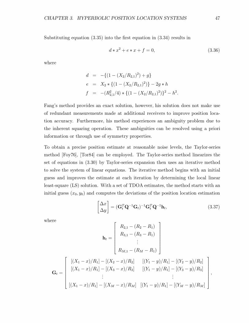
Substituting equation (3.35) into the first equation in (3.34) results in

d ∗ x2 + e ∗ x+ f = 0, (3.36)

where

d = −{(1− (X2/R2,1)2) + g}

e = X2 ∗ {(1− (X2/R2,1)2)} − 2g ∗ h

f = −(R22,1/4) ∗ {(1− (X2/R2,1)2)}2 − h2.

Fang’s method provides an exact solution, however, his solution does not make use

of redundant measurements made at additional receivers to improve position loca-

tion accuracy. Furthermore, his method experiences an ambiguity problem due to

the inherent squaring operation. These ambiguities can be resolved using a priori

information or through use of symmetry properties.

To obtain a precise position estimate at reasonable noise levels, the Taylor-series

method [Foy76], [Tor84] can be employed. The Taylor-series method linearizes the

set of equations in (3.30) by Taylor-series expansion then uses an iterative method

to solve the system of linear equations. The iterative method begins with an initial

guess and improves the estimate at each iteration by determining the local linear

least-square (LS) solution. With a set of TDOA estimates, the method starts with an

initial guess (x0, y0) and computes the deviations of the position location estimation[∆x

∆y

]= (GT

t Q−1Gt)−1GT

t Q−1ht, (3.37)

where

ht =

R2,1 − (R2 −R1)

R3,1 − (R3 −R1)...

RM,1 − (RM −R1)

Gt =

[(X1 − x)/R1]− [(X2 − x)/R2] [(Y1 − y)/R1]− [(Y2 − y)/R2]

[(X1 − x)/R1]− [(X3 − x)/R3] [(Y1 − y)/R1]− [(Y3 − y)/R3]...

...

[(X1 − x)/R1]− [(XM − x)/RM ] [(Y1 − y)/R1]− [(YM − y)/RM ]

,


and Q is the covariance matrix of the estimated TDOA’s. The values Ri for i =

1, 2, . . . ,M are computed from (3.29) with x = x0 and y = y0. In the next iteration,

x0 and y0 are set to x0 + ∆x and y0 + ∆y. The whole process is repeated until ∆x

and ∆y are sufficiently small, resulting in the estimated PL of the source (x, y). This

Taylor-series method can provide accurate results, however, it requires a close initial

guess (x0, y0) to guarantee convergence and can be very computationally intensive.

Friedlander’s method [Fri87] utilizes a Least Squares (LS) and Weighted LS (WLS)

error criterion to solve for the position location [Fri87]. He first transforms the linear

set of equations of (3.33) into

Xi,1x+ Yi,1y =1

2(X2

i + Y 2i −X2

1 − Y 21 −R2

i,1)−Ri,1R1, (3.38)

then realizes this equation in matrix form as

Sx = u−R1p, (3.39)

where

S =

Xi,1 Yi,1

......

XM,1 YM,1

x = [x y]T

u =1

2

X2i + Y 2

i −X21 − Y 2

1 −R2i,1

......

X2M + Y 2

M −X21 − Y 2

1 −R2M,1

p = [Ri,1 . . .RM,1]

T .

In order to eliminate the second term of 3.39, which requires knowledge of the un-

known term R1, the equation in (3.39) is premultiplied by a matrix N which has p

in its null-space. Matrix N is defined as

N = (I− Z)D, (3.40)

where

D = (diag{p})−1 =

Ri,1 0. . .

. . .

0 RM,1

−1


Z =

0 1. . .

. . .

. . . 1

1 0

,

and I is an identity matrix. By using singular value decomposition (SVD) on (I− Z),

Friedlander eliminates the unknown R1 parameter. The SVD of (I− Z) is given as

(I− Z) = [Uk,uk]

ηk1 0. . .

ηkM−2

0 0

[Vk,vTk ], (3.41)

where {ηk1 , . . . , ηkM−2} are the non-zero singular values. The matrix to eliminate the

second term of (3.39) is then given by

N = VTk D, (3.42)

and a closed form solution for the coordinates of the source is found by solving

NSx = Nu, (3.43)

which results in (M−2) linear equations in x and y. The source position can then be

computed using the LS solution. A closed form solution which can be used is given

by Friedlander as

x = (STNNTS)−1STNNTu. (3.44)

Friedlander also uses the Weighted Least Squares (WLS) solution, which provides the

ML estimate in the case of zero-mean Gaussian range difference noises with unequal

variance. The optimal weighting matrix is given as

W = {N(diag{p}+R1I)Q(diag{p}+R1I)NT}−1, (3.45)

where Q is the covariance matrix of the range difference equations. The weighting

matrix W is a function of the unknown parameter R1 , which can be estimated from

R1 =pTPu

pTPp, (3.46)

where

P = I− S(STS)−1S.


The resulting WLS solution is in the form

W1/2Nx = W1/2Nu, (3.47)

which results in a position location estimation by

x = (STNWNTS)−1STNWNTu. (3.48)

Friedlander’s simulation results indicated that, when using four base stations, the LS

and WLS solutions were identical. However, for more than four base stations, the

WLS PL solution outperformed the LS PL solution.

The spherical-intersection (SX) method [Sch87], [Smi87b] is another commonly used

approach. It assumes that R1 is known and solves x and y in terms of R1 from (3.33).

The least squares solution of (3.29) is then used to find the R1 and hence x and y.

Since R1 is assumed to be constant in the first step, the degree of freedom to minimize

the second norm of the error vector, ψ , used in the solution is reduced [Cha94]. The

solution obtained is therefore suboptimal as demonstrated in [Smi87a] and [Abe87].

Another approach called the spherical-interpolation (SI) method [Abe87], [Smi87a],

[Smi87b], first solves x and y in terms of R1, then inserts the intermediate result

back into (3.33) to generate equations in the unknown R1 only. Substituting the

computed R1 values that minimizes the LS equation error to the intermediate result

produces the final result. One drawback to the SI method is it inability to produce

a solution if the number of unknowns is equal to the number of equations based on

the TDOA estimates, which may occur in certain situations. The SI method was

shown in [Smi87a] to provide an order of magnitude greater noise immunity than the

SX method. Although the SI performs better than the SX method, it assumes that

the three variables x, y and R1 in (3.33) to be independent and eliminates R1 from

those equations. Consequently, the solution is suboptimal because this relationship

is ignored. The method proposed by Friedlander and the SI method have be shown

in [Fri87] to be mathematically equivalent.

A divide and conquer (DAC) method, proposed by Abel [Abe90], consists of dividing

the TDOA measurements into groups, each having a size equal to the number of

unknowns. Solution of the unknowns is calculated for each group, then appropriately

combined to provide a final solution. Although this method can achieve optimum


performance, the solution uses stochastic approximation and requires that the Fisher

information be sufficiently large. The Fisher information matrix (FIM) is the inverse

of the Cramer-Rao Matrix Bound (CRMB)(i.e.(FIM)=(CRMB)−1) [Hah75]. The

estimator provides optimum performance when the errors are small, thus implying

a low-noise threshold in which the method deviates from the CRLB. This method

requires an equal number of range difference measurements in each group, and as a

result, the TDOA estimates from the remaining sensors cannot be used to improve

accuracy.

An non-iterative solution to the hyperbolic position estimation problem which is

capable of achieving optimum performance for arbitrarily placed sensors was proposed

by Chan [Cha94]. The solution is in closed-form and valid for both distant and close

sources. When TDOA estimation errors are small, this method is an approximation

to the maximum likelihood (ML) estimator. Chan’s method performs significantly

better than the SI method and has a higher noise threshold that the DAC method

before the performance deviates from the Cramer-Rao lower bound. Furthermore, it

provides an explicit solution form that is not available in the Taylor-series method.

Following Chan’s method [Cha94], for a three base station system (M=3), producing

two TDOA’s, x and y can be solved in terms of R1 from (3.33). The solution is in

the form of[∆x

∆y

]= −

X2,1 Y2,1

X3,1 Y3,1

−1

×[R2,1

R3,1

]R1 +

1

2

R22,1 −K2 +K1

R23,1 −K3 +K1

, (3.49)

where

K1 = X21 + Y 2

1

K2 = X22 + Y 2

2

K3 = X23 + Y 2

3 .

When (3.49) is inserted into (3.29), with i = 1, a quadratic equation in terms of R1 is

produced. Substituting the positive root back into (3.49) results in the final solution.

There may exist two positive roots from the quadratic equation that can produce

two different solutions, resulting in an ambiguity. This problem can be resolved by

using a priori information. The answer to this method is the same as the spherical-

intersection method (SX) given in [Sch87].


For four or more base stations, the PL system is overdetermined because there are

more measurements of TDOA than the number of unknowns. The original set of

nonlinear TDOA equations are transformed into another set of linear equations with

an extra variable. A weighted linear LS provides an initial solution and a second

weighted LS gives an improved position estimate through the use of the known con-

strain of the source coordinates and the extra variable. Letting za = [zTp , R1]T be the

unknown vector, where zp = [x, y]T , the error vector ψ, with TDOA noise, derived

from (3.33) is

ψ = h −Gaz0a, (3.50)

where

h =1

2

R2

2,1 −X22 − Y 2

2 +X21 + Y 2

1

R23,1 −X2

3 − Y 23 +X2

1 + Y 21

...

R2M,1 −X2

M − Y 2M +X2

1 + Y 21

Ga = −

X2,1 Y2,1 R2,1

X3,1 Y3,1 R3,1

......

...

XM,1 YM,1 RM,1

.

Denoting the noise free value of {∗} as {∗}0, when di,j = d0i,j + ni,j is used to express

Ri,1 as R0i,1 + cni,1 and noting from (3.30) that R0

i = R0i,1 +R0

i , the error vector ψ is

found to be

ψ = cBn + 0.5c2n� n (3.51)

B = diag{R02, R

03, . . . , R

0M},

where � represents the Schur product. The TDOA estimates found by the general

cross-correlation methods with Gaussian data is asymptotically normally distributed

when the signal to noise (SNR) is high [Car81]. Consequently, the noise vector n

is also asymptotically normal and the covariance matrix of the error vector can be

evaluated. In practice, the condition cni,1 � R0i is usually satisfied and the second

term on the right of (3.51) can be ignored. Therefore, the error vector ψ becomes a

Gaussian random vector with covariance matrix given by

Ψ = E[ψψT ] = c2BQB (3.52)


where Q is the TDOA covariance matrix. The elements of za are related by (3.29),

which means that (3.50) is still a set of nonlinear equations in x and y variables.

The approach to solving this nonlinear problem is to first assume that there is no

relationship between x, y and R1. They can then be solved by a least squares esti-

mation. The final solution is obtained by imposing the known relationship (3.29) to

the result via another LS computation. This two step procedure is an approximation

of a true ML estimator for the source location. By considering the elements of za

independent, the ML estimate of za is

za = arg min{(h−Gaza)TΨ−1(h−Gaza)} (3.53)

= (GTa Ψ−1Ga)

−1GTaΨ−1h,

which is the generalized LS solution of (3.50). The equation of (3.53) cannot be solved

because Ψ is not known since B contains the true distances between the source and the

sensors. Further approximation is necessary in order to make the problem solvable.

When the source is far away, each R0i for i=2,3,4,...,M is close to R0 so that B ≈ R0I,

where R0 designates the range and I is the identity matrix size (M-1). Since scaling

of Ψ does not affect the answer, an approximation of (3.53) is

za ≈ (GTaQ−1Ga)

−1GTaQ−1h. (3.54)

If the source is close, (3.54) is used first to obtain an initial solution to estimate B.

The final answer is then computed from (3.53). Although (3.53) can be iterated to

provide an even better answer, simulations show that applying (3.53) once is sufficient

to give an accurate answer.

The covariance of position estimate za is obtained by evaluating the expectations of za

and zazTa from (3.53), however this is difficult because Ga contains random quantities

ri,1. The covariance matrix is computed by using a perturbation approach. In the

presence of noise

Ri,1 = R0i,1 + c ni,1. (3.55)

The matrix Ga and vector h can be expressed as Ga = G0a + ∆Ga and h = h0 + ∆h.

Since G0az

0a = h0, (3.50) implies that

ψ = ∆h−∆Gaz0a. (3.56)


Letting za = z0a + ∆za. Then from (3.53)

(G0Ta + ∆GT

a )Ψ−1(G0a + ∆Ga)(z

0a + ∆za) = (G0T

a + ∆GTa )Ψ−1(h + ∆h). (3.57)

Retaining only the linear perturbation terms and then using (3.51) and (3.56), ∆za

and its covariance matrix is

∆za = c(GTaΨ−1Ga)

−1GTaΨ−1Bn (3.58)

cov(za) = E[∆za∆zTa ] = (G0Ta Ψ−1G0

a)−1,

where the square error term in (3.51) has been ignored and (3.52) has been used to

give cov(za).

The position estimation za assumes x, y and Ri are independent; however, they are

related by (3.29). Therefore, we can incorporate this relationship to get an improved

estimate. When the bias is ignored because of small errors in the TDOA estimates, the

vector za is a random vector with its mean centered at the true value with covariance

matrix (3.58). Hence the elements of za can be expressed as

za,1 = x0 + e1, za,2 = y0 + e2, za,3 = R01 + e1, (3.59)

where e1, e2 and e3 are the estimation errors of za . Subtracting the first two elements

of za by X1 and Y1, and then squaring the elements gives another set of equations

ψ′= h

′ −G′az′0a , (3.60)

where ψ′

is a vector denoting the inaccuracies in za. Substituting (3.59) into (3.60)

results in

Ψ′1 = 2(x0 −X1)e1 + e2

1 ≈ 2(x0 −X1)e1

Ψ′2 = 2(y0 − Y1)e2 + e2

2 ≈ 2(y0 − Y1)e2 (3.61)

Ψ′3 = 2R0

1e3 + e23 ≈ 2R0

1e3.

The approximation to the ML procedure used here is valid only if the errors ei are

small. The covariance matrix of ψ′

is given by

Ψ′

= [ψ′ψ′T ]4B

′cov(za)B

′(3.62)

B′

= diag{x0 −X1, y0 − Y1, R

01}.


Since ψ is Gaussian, then it follows that ψ′

is also Gaussian, thus the ML estimate

of z′a is

z′a = (G

′Ta Ψ

′−1G′a)−1G

′Ta Ψ

′−1h′. (3.63)

The matrix Ψ′is not known since it contains the true values of the position. Neverthe-

less, B′

can be approximated by using the values za and G0a in (3.58) approximated

by Ga and B in (3.52) approximated by the values computed from (3.54).

If the source is distant, then the covariance matrix can be approximated as

cov(za) ≈ c2R02

(G0Ta Q−1G0

a)−1, (3.64)

and (3.63) reduces to

z′a ≈ (G

′Ta B

′−1GaQ−1GaB

′−1G′a)−1(G

′Ta B

′−1GaQ−1GaB

′−1G′a)h

′. (3.65)

Matrix G′a is constant. By taking the expectations of z

′a and z

′az′Ta , the covariance

matrix of z′a is

cov(z′a) = (G

′Ta Ψ

′−1G′a)−1. (3.66)

Finally, the position location estimation is obtained from as

zp =√

z′a +

X1

Y1

(3.67)

or

zp = −√

z′a +

X1

Y1

.The proper solution is selected to be the one which lies in the region of interest. If

one of the coordinates of z′a is close to zero, the square root in (3.67) may become

imaginary. If this occurs, the imaginary component is set to zero. The covariance

matrix of the position location estimate can be determined from z′a in (3.60), with

x = x0 + ex and y = y0 + ey. Thus from (3.60)

z′a,1 − (x0 −X1)2 = 2(x0 −X1)ex + e2

x (3.68)

z′a,2 − (y0 − Y1)2 = 2(y0 − Y1)ey + e2

y.

The errors ex and ey are relatively small compared to x0 and y0, thus we can eliminate

e2x and e2

y. Then using (3.52), (3.58) , (3.62) and (3.67), the covariance matrix, Φ, of


position location estimate, zp,is found to be

Φ = cov(zp) =1

4B′′−1cov(z

′a)B

′′−1 (3.69)

= c2(B′′G′Ta B

′−1G0Ta B−1Q−1B−1G0

aB′−1G

′aB′′)−1,

where

B′′

=

(x0 −X1) 0

0 ((y0 − Y1)

.To summarize Chan’s method, the location of a distant source can be estimated by

using equations (3.54), (3.65) and (3.67). The covariance matrix of the PL estimate

is determined from (3.69). For locating near sources, (3.54) is used to give an approx-

imation of B, then used in (3.53), (3.63) and (3.67) to produce a PL solution. The

covariance matrix of the PL estimates can then be determined from (3.69). Chan’s

method offers a closed form solution which can achieve the CRLB. However, it does

so when the range difference errors are assumed to be small. His method also requires

a priori knowledge of the approximate location and distance of the source to resolve

ambiguities in the PL solution.

The hyperbolic PL estimation algorithms presented offer different accuracy’s and

complexities. The Taylor-series LS method offers accurate position location estima-

tion at reasonable noise levels and is applicable to any number of range difference

measurements, but can be computational intensive. Fang’s method provides an op-

timal solution when the system of equations is consistent but does not make use of

redundant measurements. Friedlander’s approach reduces the computational require-

ments for the solution but does is suboptimal because it eliminates a fundamental

relationship. Chan’s method offers a closed form solution, thus eliminating the need

for an iteration approach, but requires a priori information to eliminate ambiguities.

The optimal PL algorithm for a given situation depends on the geometrical configu-

ration of the base stations, the number of coordinates of the source to be solved and

range difference measurements utilized, computational requirements and complexity,

assumptions on the statistical nature of the channel and desired accuracy.


3.4 Measures of Position Location Accuracy

A set of benchmarks is required to evaluate the accuracy of the hyperbolic position

location technique. A commonly used measure of PL accuracy is the comparison of

the mean square error (MSE) of the position location solution to the theoretical MSE

based on the Cramer-Rao Lower Bound (CRLB). Another commonly used measure

of PL accuracy is the circle of error probability (CEP). The effect of the geometric

configuration of the base stations on the accuracy of the position location estimate

is measured by the geometric dilution of precision (GDOP). A simple relationship

exists between the GDOP and CEP measures. Lee in [Lee75a] and [Lee75b] provides

a novel procedure for assessing the accuracy of hyperbolic multilateration PL systems

and limitations of the accuracy’s. Hepsaydir and Yates provide a performance analysis

of position locationing systems using existing CDMA networks in [Hep94].

3.4.1 MSE and the Cramer-Rao Lower Bound

A commonly used measure of accuracy of a PL estimator is the comparison of the

mean squared error (MSE) of the PL solution to the theoretical MSE based on the

Cramer-Rao Lower Bound on the variance of unbiased estimators. The classical

method for computing the MSE of a 2-D position location estimate is

MSE = ε = E[(x− x)2 + (y − y)2], (3.70)

where (x, y) is the coordinates of the source and (x, y) is the estimated position of

the source. The root-mean square (RMS) position location error, which can also be

used as a measure of PL accuracy, is calculated as the square root of the MSE

RMS =√ε =

√E[(x− x)2 + (y − y)2]. (3.71)

To gauge the accuracy of the PL estimator, the calculated MSE or RMS PL is com-

pared to the theoretical MSE based on the Cramer-Rao Lower Bound (CRLB). The

conventional CRLB sets a lower bound for the variance of any unbiased parameter

estimator and is typically used for a stationary Gaussian signal in the presence of

stationary Gaussian noise [Gar92b]. For non-Gaussian and nonstationary (cyclosta-

tionary) signals and noise, alternate methods have been used to evaluate the perfor-

mance of the estimators [Gar92b]. The derivation of the CRLB for Gaussian noise is


provided in [Cha94], [Kna76], [Hah73] and [Hah75]. The CRLB on the PL covariance

is given by Chan [Cha94] as

Φ = c2(GTt Q−1Gt)

−1, (3.72)

where Gt is defined in (3.37) with (x, y, Ri) = (x0, y0, R0i ), which are the actual

coordinates of the source and the range of the first base station to the source, and

matrix Q is the TDOA covariance matrix. The sum of the diagonal elements of Φ

defines the theoretical lower bound on the MSE of the PL estimator. Matrix Q may

not be known in practice; however, if the noise power spectral densities are similar

at the receivers, it can be replaced be a theoretical TDOA covariance matrix with

diagonal elements of σ2d and 0.5σ2

d for all other elements, where σ2d is the variance of

the TDOA estimate [Cha94].

3.4.2 Circular Error Probability

A crude but simple measure of accuracy of position location estimates that is com-

monly used is the circular error probability (CEP) [Tor84] [Foy76]. The CEP is a

measure of the uncertainty in the location estimator relative to its mean. For a 2-D

system, the CEP is defined as the radius of a circle which contains half of the real-

izations of the random vector with the mean as its center. If the position location

estimator is unbiased, the CEP is a measure of the uncertainty relative to the true

transmitter position. If the estimator is biased and bound by bias B, then with a

probability of one-half, a particular estimate is within a distance B + CEP from the

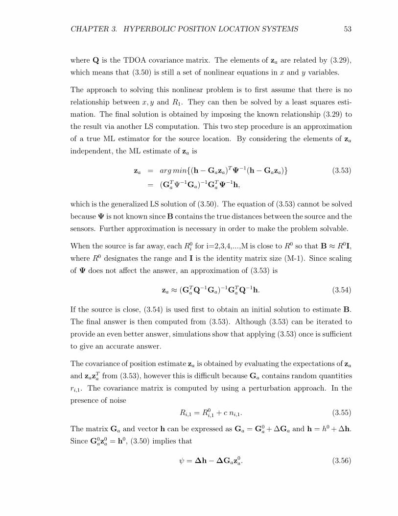
true transmitter position. Figure 3.2 illustrates the 2-D geometrical relations.

The CEP is a complicated function and is usually approximated. Details of its compu-

tation can be found in [Foy76] and [Tor84]. For hyperbolic position location estimator

the CEP is approximated with an accuracy within approximately 10 % as

CEP ≈ 0.75√σ2x + σ2

y, (3.73)

where σ2x and σ2

y are the variances in the estimated position [Tor84].


Figure 3.2: Circle of Error Probability

3.4.3 Geometric Dilution of Precision

The accuracy of Range-Based PL systems depends to a large extent on the geometric

relationship between the base stations and the source to be located. One measure that

quantifies the accuracy based on this geometric configuration is called the geometric

dilution of precision (GDOP) [Wel86] [Tor84] [Ban85] [Lee75a]. The GDOP is defined

as the ratio of the RMS position error to the RMS ranging error. The GDOP for an

unbiased estimator and a ranging system is given by [Jor84] as

GDOP =√tr[(ATA)−1], (3.74)

where A is express in equation (3.20) and tr indicates the trace of the resulting

matrix. The GDOP for an unbiased estimator and a 2-D hyperbolic system is given

by [Tor84] and [Lee75a] as

GDOP =(√

(cσx)2 + (cσy)2)/√

(cσs)2 (3.75)

=(√

σ2x + σ2

y

)/σs,

where (cσs)2 is the mean squared ranging error and (cσx)2 and (cσy)2 are the mean

square position errors in the x and y estimates. The GDOP is related to the CEP by

CEP ≈ (0.75σs)GDOP. (3.76)

The GDOP can be used as a criterion for selecting a set of base station from a large

set whose measurements produce minimum PL estimation error or for designing base

station location within new systems.


3.5 Chapter Summary

This chapter introduced the TDOA estimation techniques and hyperbolic PL al-

gorithms used in the hyperbolic position location method. A general model for

the TDOA estimation problem was developed and the generalized cross-correlation

(GCC) techniques commonly used for time delay estimation were presented. The

effect of the frequency functions on the TDOA estimation and the importance of the

choice of frequency function was discussed. Although GCC methods do facilitate

the estimation of the TDOA, they do encounter problems which are critical to the

position location problem. Firstly, GCC require the differences in the TDOA for

each signal to be greater than the widths of the cross-correlation functions so that

the correlation peaks can be resolved. If not separated sufficiently, overlapping of

cross-correlation functions corrupt the TDOA estimate. Furthermore, because GCC

methods are not signal-selective, they produce correlation peaks for all signals and

are faced with the problem of identifying the TDOA estimate of interest. Signal-

selective TDOA estimation techniques outperform GCC methods; however, they do

not offer any advantages over GCC methods when the spectrally overlapping noise

and interference exhibit the same cycle frequency as the signal of interest, which is

encountered in multiuser CDMA systems.

A general range difference position location model was formulated and the hyperbolic

algorithms used to provide solutions to the range difference equations were presented.

For the problem of geolocating mobile units within a cellular infrastructure, the algo-

rithms applicable to arbitrarily placed base station were reviewed. Fang’s PL method,

Friedlanders Least Square (LS) and Weighted LS PL method, the iterative Taylor-

series LS PL method and Chan’s closed form PL method were described in detail. The

advantages and disadvantages of the various PL algorithms were discussed. Finally,

the measures of position location accuracy commonly used to evaluate hyperbolic

position location algorithms were reviewed.

Chapter 3 Hyperbolic Position Location Systems location... · 2006-02-01 · CHAPTER 3. HYPERBOLIC...

Documents

Transcript of Chapter 3 Hyperbolic Position Location Systems location... · 2006-02-01 · CHAPTER 3. HYPERBOLIC...