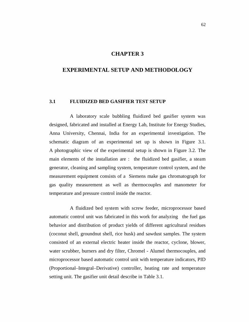
62

CHAPTER 3

EXPERIMENTAL SETUP AND METHODOLOGY

3.1 FLUIDIZED BED GASIFIER TEST SETUP

A laboratory scale bubbling fluidized bed gasifier system was

designed, fabricated and installed at Energy Lab, Institute for Energy Studies,

Anna University, Chennai, India for an experimental investigation. The

schematic diagram of an experimental set up is shown in Figure 3.1.

A photographic view of the experimental setup is shown in Figure 3.2. The

main elements of the installation are : the fluidized bed gasifier, a steam

generator, cleaning and sampling system, temperature control system, and the

measurement equipment consists of a Siemens make gas chromatograph for

gas quality measurement as well as thermocouples and manometer for

temperature and pressure control inside the reactor.

A fluidized bed system with screw feeder, microprocessor based

automatic control unit was fabricated in this work for analyzing the fuel gas

behavior and distribution of product yields of different agricultural residues

(coconut shell, groundnut shell, rice husk) and sawdust samples. The system

consisted of an external electric heater inside the reactor, cyclone, blower,

water scrubber, burners and dry filter, Chromel - Alumel thermocouples, and

microprocessor based automatic control unit with temperature indicators, PID

(Proportional–Integral–Derivative) controller, heating rate and temperature

setting unit. The gasifier unit detail describe in Table 3.1.

63

1 control panel; 2 air blower; 3 Variable displacement drive motor; 4 biomass

hopper; 5 steam generator; 6 Thermo couple; 7 free board; 8 Suction blower;

9 flare; 10 cyclone; 11 blower motor; 12 water scrubber; 13 water inlet; 14 to

gas analyser; 15 burner; 16 dry filter; 17 fluidized bed gasifier

Figure 3.1 Experimental uidized bed gasi cation system

64

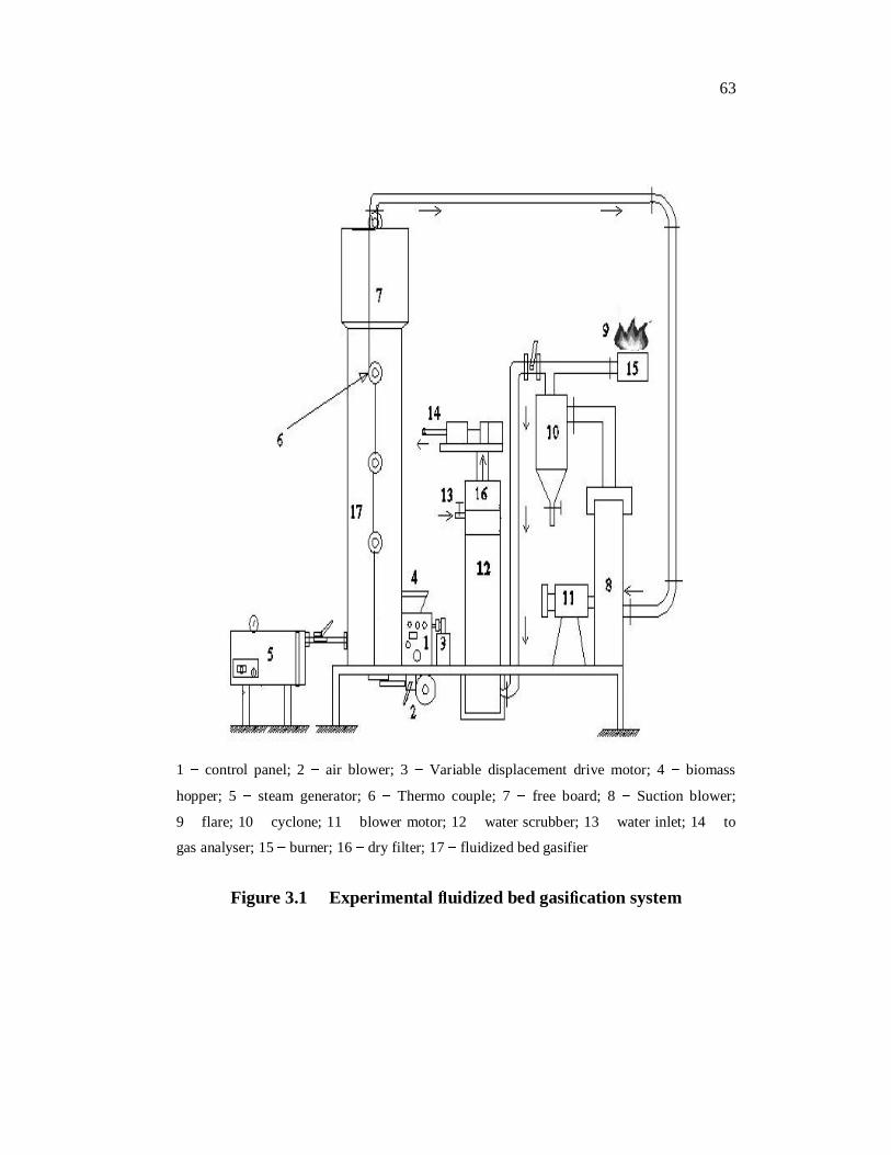
Table 3.1 Main design and operating features of the bubbling

fluidized bed gasifier

Type of gasifier Bubbling fluidized bedGeometrical parameters ID: 108 mm; total height :1400 mmHeating Type External electric heatingCooling medium WaterFeedstock capacity 5-20 kg / h (depending on the type of fuel)Feeding equipment Screw feederGasifying agents Air, SteamOperating temperature 650 - 950 ºCHeating rate 1-60°C/minFeed stock Coconut shell, groundnut shell, rice husk,

and saw dustMain process variables Reactor temperature, steam to Biomass ratioFuel gas treatments Cyclone, Water scrubber, Dry filter

The details of various components, fabrication details, preparation

of samples and its properties, experimental procedures are discussed in this

chapter. The heating coils were wired at the centre of the furnace and it was

insulated with ceramic fiber blankets to prevent the heat loss from the heating

coil to atmosphere. The ceramic fiber layer was covered with mild steel sheets

as an outer cover. 310 grade stainless steel pipes were used as reactor for

heating the samples.

The details of components of the bubbling fluidized bed gasifierhave been developed are explained here.

65

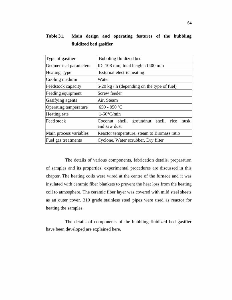
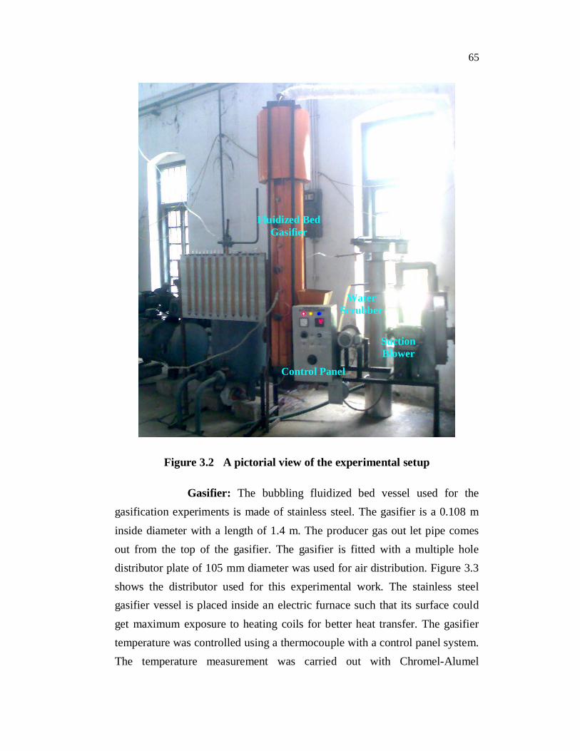
Figure 3.2 A pictorial view of the experimental setup

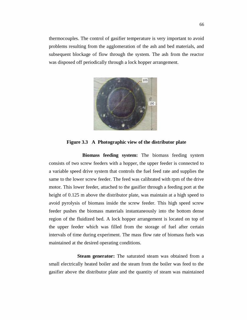
Gasifier: The bubbling fluidized bed vessel used for thegasification experiments is made of stainless steel. The gasifier is a 0.108 minside diameter with a length of 1.4 m. The producer gas out let pipe comesout from the top of the gasifier. The gasifier is fitted with a multiple holedistributor plate of 105 mm diameter was used for air distribution. Figure 3.3shows the distributor used for this experimental work. The stainless steelgasifier vessel is placed inside an electric furnace such that its surface couldget maximum exposure to heating coils for better heat transfer. The gasifiertemperature was controlled using a thermocouple with a control panel system.The temperature measurement was carried out with Chromel-Alumel

Fluidized BedGasifier

WaterScrubber

SuctionBlower

Control Panel

66

thermocouples. The control of gasifier temperature is very important to avoidproblems resulting from the agglomeration of the ash and bed materials, andsubsequent blockage of flow through the system. The ash from the reactorwas disposed off periodically through a lock hopper arrangement.

Figure 3.3 A Photographic view of the distributor plate

Biomass feeding system: The biomass feeding systemconsists of two screw feeders with a hopper, the upper feeder is connected toa variable speed drive system that controls the fuel feed rate and supplies thesame to the lower screw feeder. The feed was calibrated with rpm of the drivemotor. This lower feeder, attached to the gasifier through a feeding port at theheight of 0.125 m above the distributor plate, was maintain at a high speed toavoid pyrolysis of biomass inside the screw feeder. This high speed screwfeeder pushes the biomass materials instantaneously into the bottom denseregion of the fluidized bed. A lock hopper arrangement is located on top ofthe upper feeder which was filled from the storage of fuel after certainintervals of time during experiment. The mass flow rate of biomass fuels wasmaintained at the desired operating conditions.

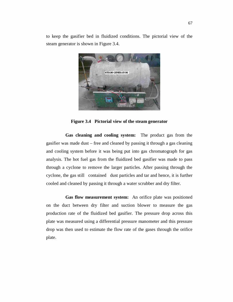
Steam generator: The saturated steam was obtained from asmall electrically heated boiler and the steam from the boiler was feed to thegasifier above the distributor plate and the quantity of steam was maintained

67

to keep the gasifier bed in fluidized conditions. The pictorial view of thesteam generator is shown in Figure 3.4.

Figure 3.4 Pictorial view of the steam generator

Gas cleaning and cooling system: The product gas from the

gasifier was made dust – free and cleaned by passing it through a gas cleaning

and cooling system before it was being put into gas chromatograph for gas

analysis. The hot fuel gas from the fluidized bed gasifier was made to pass

through a cyclone to remove the larger particles. After passing through the

cyclone, the gas still contained dust particles and tar and hence, it is further

cooled and cleaned by passing it through a water scrubber and dry filter.

Gas flow measurement system: An orifice plate was positioned

on the duct between dry filter and suction blower to measure the gas

production rate of the fluidized bed gasifier. The pressure drop across this

plate was measured using a differential pressure manometer and this pressure

drop was then used to estimate the flow rate of the gases through the orifice

plate.

68

3.2 PROCESS INSTRUMENTATION AND CONTROL

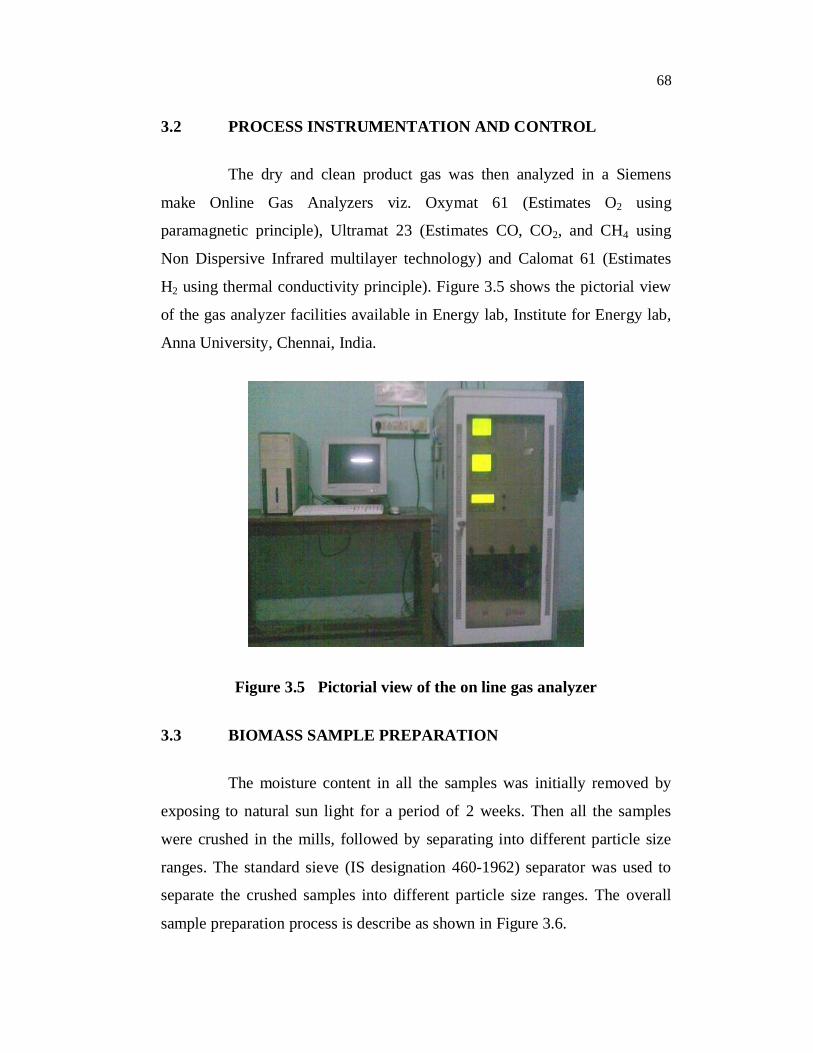
The dry and clean product gas was then analyzed in a Siemens

make Online Gas Analyzers viz. Oxymat 61 (Estimates O2 using

paramagnetic principle), Ultramat 23 (Estimates CO, CO2, and CH4 using

Non Dispersive Infrared multilayer technology) and Calomat 61 (Estimates

H2 using thermal conductivity principle). Figure 3.5 shows the pictorial view

of the gas analyzer facilities available in Energy lab, Institute for Energy lab,

Anna University, Chennai, India.

Figure 3.5 Pictorial view of the on line gas analyzer

3.3 BIOMASS SAMPLE PREPARATION

The moisture content in all the samples was initially removed by

exposing to natural sun light for a period of 2 weeks. Then all the samples

were crushed in the mills, followed by separating into different particle size

ranges. The standard sieve (IS designation 460-1962) separator was used to

separate the crushed samples into different particle size ranges. The overall

sample preparation process is describe as shown in Figure 3.6.

69

Figure 3.6 The overall sample preparation process

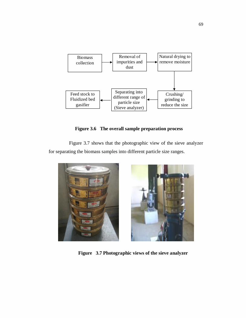
Figure 3.7 shows that the photographic view of the sieve analyzer

for separating the biomass samples into different particle size ranges.

Figure 3.7 Photographic views of the sieve analyzer

Biomasscollection

Removal ofimpurities and

dust

Natural drying toremove moisture

Crushing/grinding to

reduce the size

Separating intodifferent range of

particle size(Sieve analyzer)

Feed stock toFluidized bed

gasifier

70

3.4 SAMPLE TESTING

Compositions of the biomass samples are very essential for this

study because it influences the gasification process. Chemical composition

and structure of agricultural residues differ from crop to crop and is affected

by season, soil type and irrigation conditions. The components and elements

present with all the samples and higher heating values of the samples were

analyzed in the SGS India Pvt. limited laboratory, Chennai. The samples were

tested after crushing and natural drying process for the removal of moisture

present in the sample. Figure 3.8 shows the pictorial view of weighing

machine used for the experimental work. The carbon, hydrogen, oxygen and

nitrogen percentage were found by elemental analysis, volatile matter, fixed

carbon and moisture content were found from the component analysis. The

protocols used for analyzing the different composition of the samples are

given in Table 3.2.

Figure 3.8 Photographic view of the Weighing Machine

71

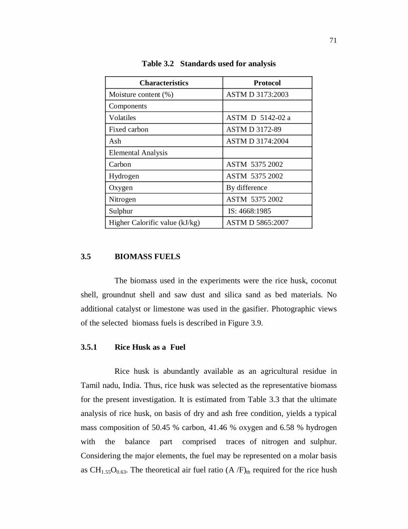
Table 3.2 Standards used for analysis

Characteristics ProtocolMoisture content (%) ASTM D 3173:2003ComponentsVolatiles ASTM D 5142-02 aFixed carbon ASTM D 3172-89Ash ASTM D 3174:2004Elemental AnalysisCarbon ASTM 5375 2002Hydrogen ASTM 5375 2002Oxygen By differenceNitrogen ASTM 5375 2002Sulphur IS: 4668:1985Higher Calorific value (kJ/kg) ASTM D 5865:2007

3.5 BIOMASS FUELS

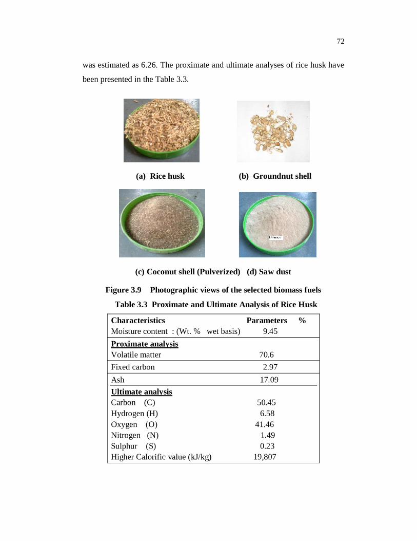
The biomass used in the experiments were the rice husk, coconut

shell, groundnut shell and saw dust and silica sand as bed materials. No

additional catalyst or limestone was used in the gasifier. Photographic views

of the selected biomass fuels is described in Figure 3.9.

3.5.1 Rice Husk as a Fuel

Rice husk is abundantly available as an agricultural residue in

Tamil nadu, India. Thus, rice husk was selected as the representative biomass

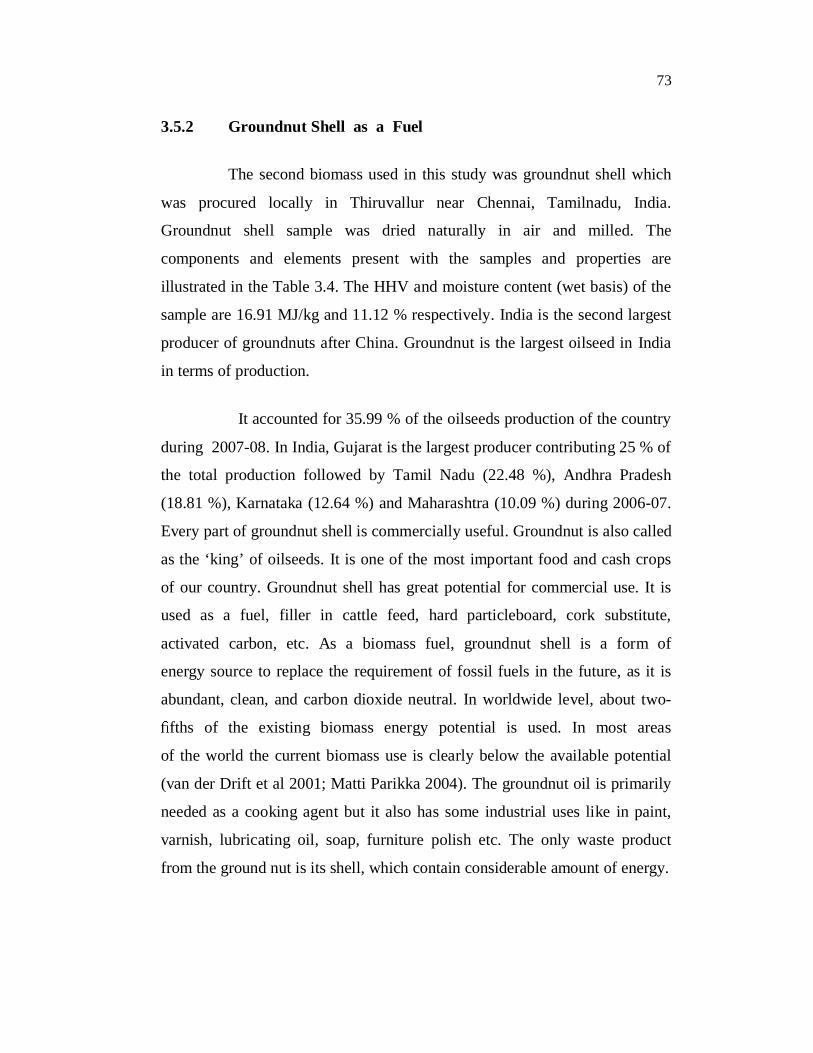
for the present investigation. It is estimated from Table 3.3 that the ultimate

analysis of rice husk, on basis of dry and ash free condition, yields a typical

mass composition of 50.45 % carbon, 41.46 % oxygen and 6.58 % hydrogen

with the balance part comprised traces of nitrogen and sulphur.

Considering the major elements, the fuel may be represented on a molar basis

as CH1.55O0.63. The theoretical air fuel ratio (A /F)th required for the rice hush

72

was estimated as 6.26. The proximate and ultimate analyses of rice husk have

been presented in the Table 3.3.

(a) Rice husk (b) Groundnut shell

(c) Coconut shell (Pulverized) (d) Saw dust

Figure 3.9 Photographic views of the selected biomass fuels

Table 3.3 Proximate and Ultimate Analysis of Rice Husk

Characteristics Parameters %Moisture content : (Wt. % wet basis) 9.45Proximate analysisVolatile matter 70.6Fixed carbon 2.97Ash 17.09Ultimate analysisCarbon (C) 50.45Hydrogen (H) 6.58Oxygen (O) 41.46Nitrogen (N) 1.49Sulphur (S) 0.23Higher Calorific value (kJ/kg) 19,807

73

3.5.2 Groundnut Shell as a Fuel

The second biomass used in this study was groundnut shell which

was procured locally in Thiruvallur near Chennai, Tamilnadu, India.

Groundnut shell sample was dried naturally in air and milled. The

components and elements present with the samples and properties are

illustrated in the Table 3.4. The HHV and moisture content (wet basis) of the

sample are 16.91 MJ/kg and 11.12 % respectively. India is the second largest

producer of groundnuts after China. Groundnut is the largest oilseed in India

in terms of production.

It accounted for 35.99 % of the oilseeds production of the country

during 2007-08. In India, Gujarat is the largest producer contributing 25 % of

the total production followed by Tamil Nadu (22.48 %), Andhra Pradesh

(18.81 %), Karnataka (12.64 %) and Maharashtra (10.09 %) during 2006-07.

Every part of groundnut shell is commercially useful. Groundnut is also called

as the ‘king’ of oilseeds. It is one of the most important food and cash crops

of our country. Groundnut shell has great potential for commercial use. It is

used as a fuel, filler in cattle feed, hard particleboard, cork substitute,

activated carbon, etc. As a biomass fuel, groundnut shell is a form of

energy source to replace the requirement of fossil fuels in the future, as it is

abundant, clean, and carbon dioxide neutral. In worldwide level, about two-

fths of the existing biomass energy potential is used. In most areas

of the world the current biomass use is clearly below the available potential

(van der Drift et al 2001; Matti Parikka 2004). The groundnut oil is primarily

needed as a cooking agent but it also has some industrial uses like in paint,

varnish, lubricating oil, soap, furniture polish etc. The only waste product

from the ground nut is its shell, which contain considerable amount of energy.

74

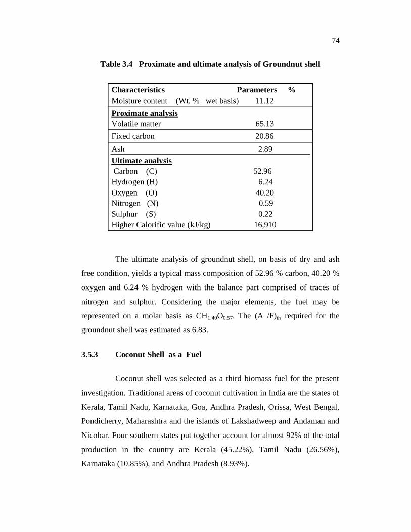
Table 3.4 Proximate and ultimate analysis of Groundnut shell

Characteristics Parameters %Moisture content (Wt. % wet basis) 11.12Proximate analysisVolatile matter 65.13Fixed carbon 20.86Ash 2.89Ultimate analysis Carbon (C) 52.96Hydrogen (H) 6.24Oxygen (O) 40.20Nitrogen (N) 0.59Sulphur (S) 0.22Higher Calorific value (kJ/kg) 16,910

The ultimate analysis of groundnut shell, on basis of dry and ash

free condition, yields a typical mass composition of 52.96 % carbon, 40.20 %

oxygen and 6.24 % hydrogen with the balance part comprised of traces of

nitrogen and sulphur. Considering the major elements, the fuel may be

represented on a molar basis as CH1.40O0.57. The (A /F)th required for the

groundnut shell was estimated as 6.83.

3.5.3 Coconut Shell as a Fuel

Coconut shell was selected as a third biomass fuel for the present

investigation. Traditional areas of coconut cultivation in India are the states of

Kerala, Tamil Nadu, Karnataka, Goa, Andhra Pradesh, Orissa, West Bengal,

Pondicherry, Maharashtra and the islands of Lakshadweep and Andaman and

Nicobar. Four southern states put together account for almost 92% of the total

production in the country are Kerala (45.22%), Tamil Nadu (26.56%),

Karnataka (10.85%), and Andhra Pradesh (8.93%).

75

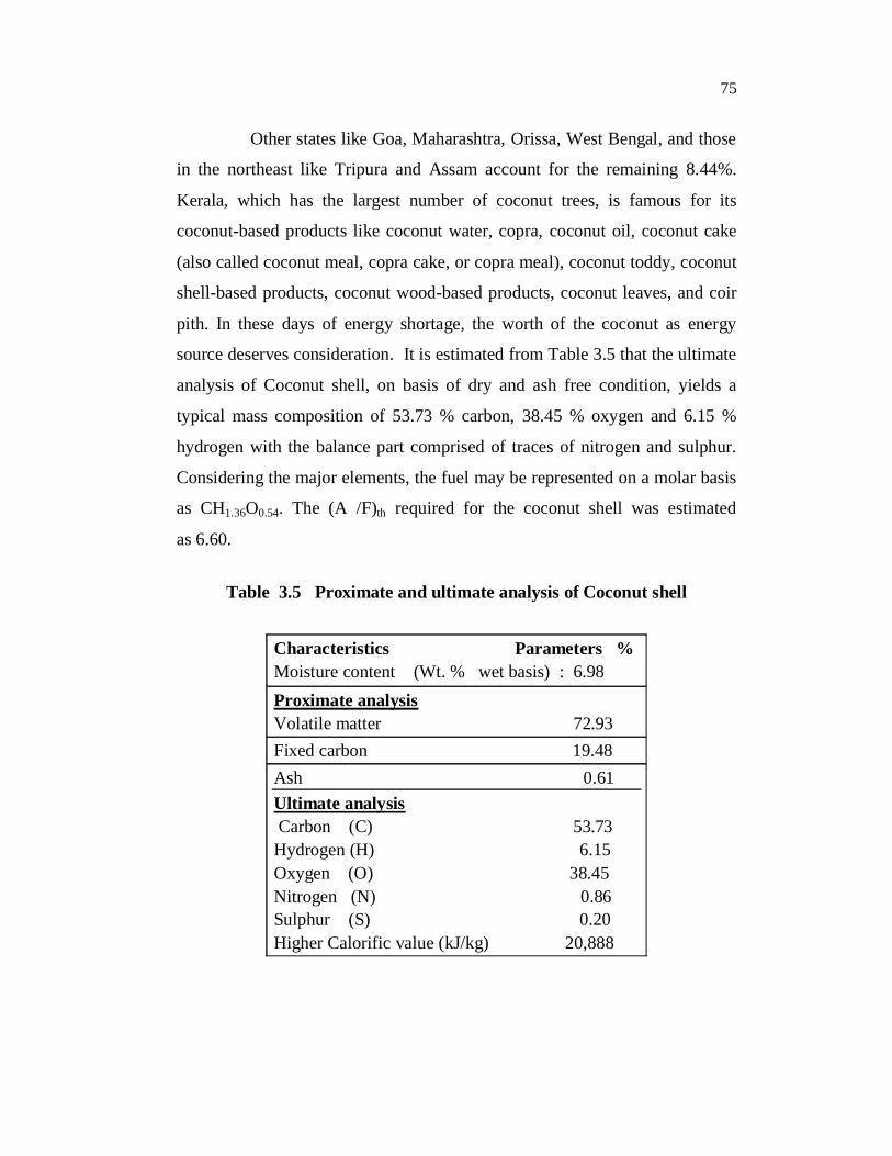
Other states like Goa, Maharashtra, Orissa, West Bengal, and those

in the northeast like Tripura and Assam account for the remaining 8.44%.

Kerala, which has the largest number of coconut trees, is famous for its

coconut-based products like coconut water, copra, coconut oil, coconut cake

(also called coconut meal, copra cake, or copra meal), coconut toddy, coconut

shell-based products, coconut wood-based products, coconut leaves, and coir

pith. In these days of energy shortage, the worth of the coconut as energy

source deserves consideration. It is estimated from Table 3.5 that the ultimate

analysis of Coconut shell, on basis of dry and ash free condition, yields a

typical mass composition of 53.73 % carbon, 38.45 % oxygen and 6.15 %

hydrogen with the balance part comprised of traces of nitrogen and sulphur.

Considering the major elements, the fuel may be represented on a molar basis

as CH1.36O0.54. The (A /F)th required for the coconut shell was estimated

as 6.60.

Table 3.5 Proximate and ultimate analysis of Coconut shell

Characteristics Parameters %Moisture content (Wt. % wet basis) : 6.98Proximate analysisVolatile matter 72.93Fixed carbon 19.48Ash 0.61Ultimate analysis Carbon (C) 53.73Hydrogen (H) 6.15Oxygen (O) 38.45Nitrogen (N) 0.86Sulphur (S) 0.20Higher Calorific value (kJ/kg) 20,888

76

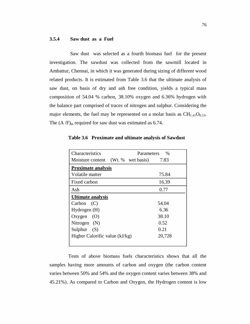
3.5.4 Saw dust as a Fuel

Saw dust was selected as a fourth biomass fuel for the present

investigation. The sawdust was collected from the sawmill located in

Ambattur, Chennai, in which it was generated during sizing of different wood

related products. It is estimated from Table 3.6 that the ultimate analysis of

saw dust, on basis of dry and ash free condition, yields a typical mass

composition of 54.04 % carbon, 38.10% oxygen and 6.36% hydrogen with

the balance part comprised of traces of nitrogen and sulphur. Considering the

major elements, the fuel may be represented on a molar basis as CH1.41O0.53.

The (A /F)th required for saw dust was estimated as 6.74.

Table 3.6 Proximate and ultimate analysis of Sawdust

Characteristics Parameters %Moisture content (Wt. % wet basis) 7.83Proximate analysisVolatile matter 75.84Fixed carbon 16.39Ash 0.77Ultimate analysisCarbon (C) 54.04Hydrogen (H) 6.36Oxygen (O) 38.10Nitrogen (N) 0.52Sulphur (S) 0.21Higher Calorific value (kJ/kg) 20,728

Tests of above biomass fuels characteristics shows that all the

samples having more amounts of carbon and oxygen (the carbon content

varies between 50% and 54% and the oxygen content varies between 38% and

45.21%). As compared to Carbon and Oxygen, the Hydrogen content is low

77

and the values are between 6% and 7%. The Sulfur content in all the samples

is very low with less than 0.25%. Which indicate that the usage of biomass

will not create any environmental related problems. The fixed carbon, ash and

moisture content vary with individual samples. The coconut shell, corncob

and sawdust having more fixed carbon and very low ash content, the

groundnut shell also contains more fixed carbon but the ash content is more

compared with both coconut shell and saw dust. The analysis show that rice

husk have very high amount of ash as compared with all other samples in this

study. Composition varies with all the samples and this will be useful for

studying the influence of different composition on gas yields.

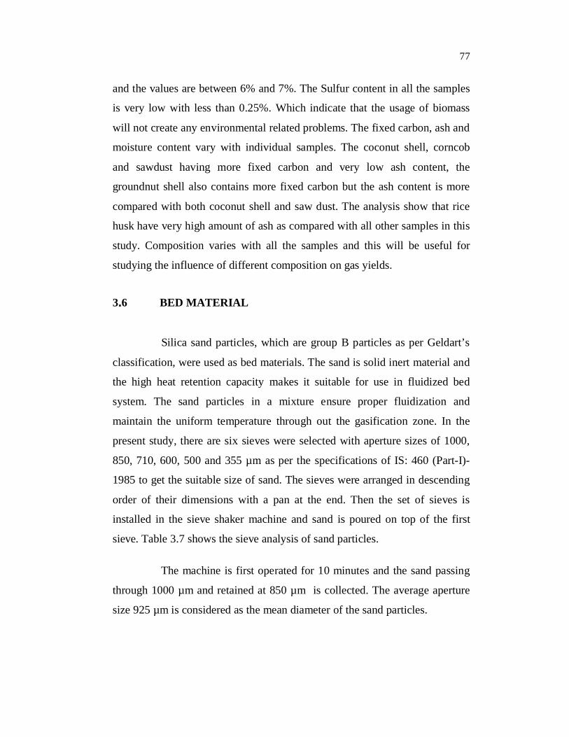
3.6 BED MATERIAL

Silica sand particles, which are group B particles as per Geldart’s

classification, were used as bed materials. The sand is solid inert material and

the high heat retention capacity makes it suitable for use in fluidized bed

system. The sand particles in a mixture ensure proper fluidization and

maintain the uniform temperature through out the gasification zone. In the

present study, there are six sieves were selected with aperture sizes of 1000,

850, 710, 600, 500 and 355 µm as per the specifications of IS: 460 (Part-I)-

1985 to get the suitable size of sand. The sieves were arranged in descending

order of their dimensions with a pan at the end. Then the set of sieves is

installed in the sieve shaker machine and sand is poured on top of the first

sieve. Table 3.7 shows the sieve analysis of sand particles.

The machine is first operated for 10 minutes and the sand passing

through 1000 µm and retained at 850 µm is collected. The average aperture

size 925 µm is considered as the mean diameter of the sand particles.

78

Table 3.7 Sieve analysis of Sand particles

Sieve aperture size

(µm)

Mass particles retained in sieve

(g)

1000 None

850 22.6

710 36.4

600 105

500 125

355 122

300 85

Total mass of samples (g) : 496

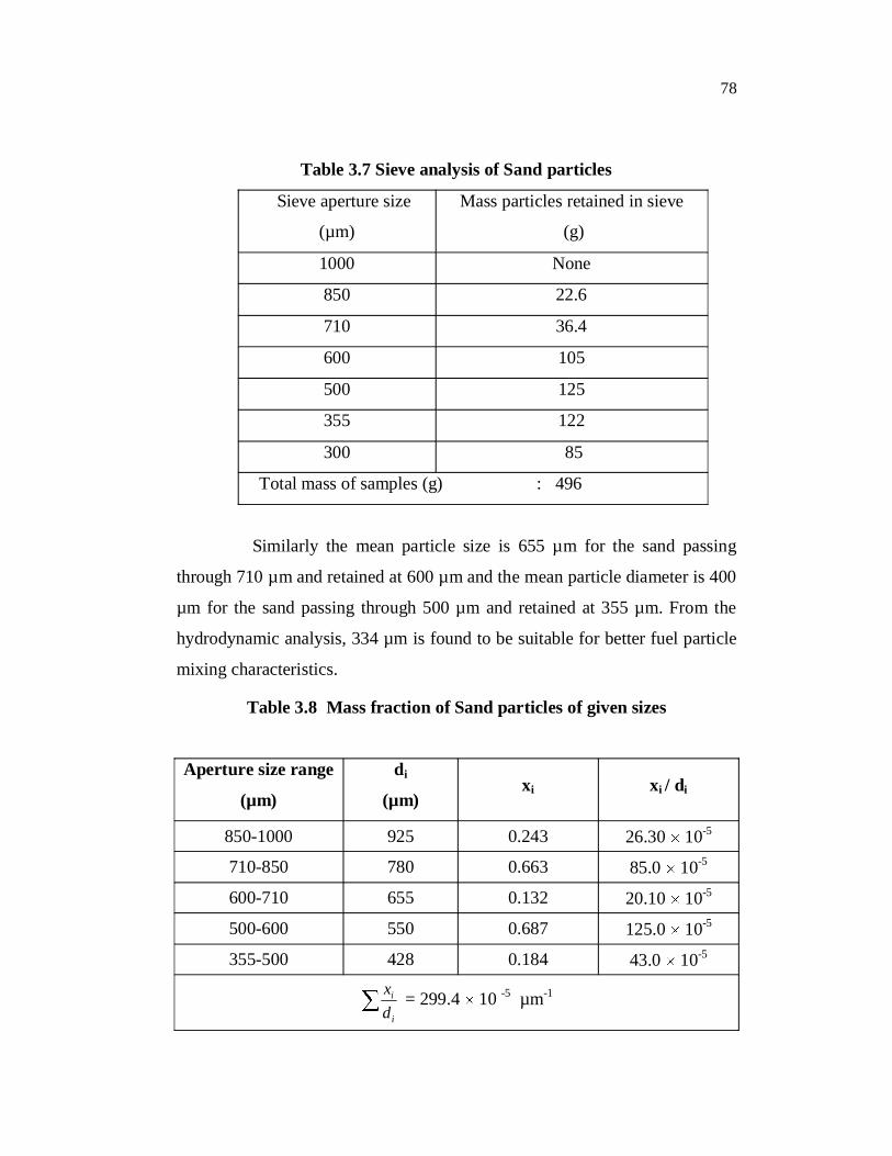
Similarly the mean particle size is 655 µm for the sand passing

through 710 µm and retained at 600 µm and the mean particle diameter is 400

µm for the sand passing through 500 µm and retained at 355 µm. From the

hydrodynamic analysis, 334 µm is found to be suitable for better fuel particle

mixing characteristics.

Table 3.8 Mass fraction of Sand particles of given sizes

Aperture size range

(µm)

di

(µm)xi xi / di

850-1000 925 0.243 26.30 10-5

710-850 780 0.663 85.0 10-5

600-710 655 0.132 20.10 10-5

500-600 550 0.687 125.0 10-5

355-500 428 0.184 43.0 10-5

i

i

dx = 299.4 10 -5 µm-1

79

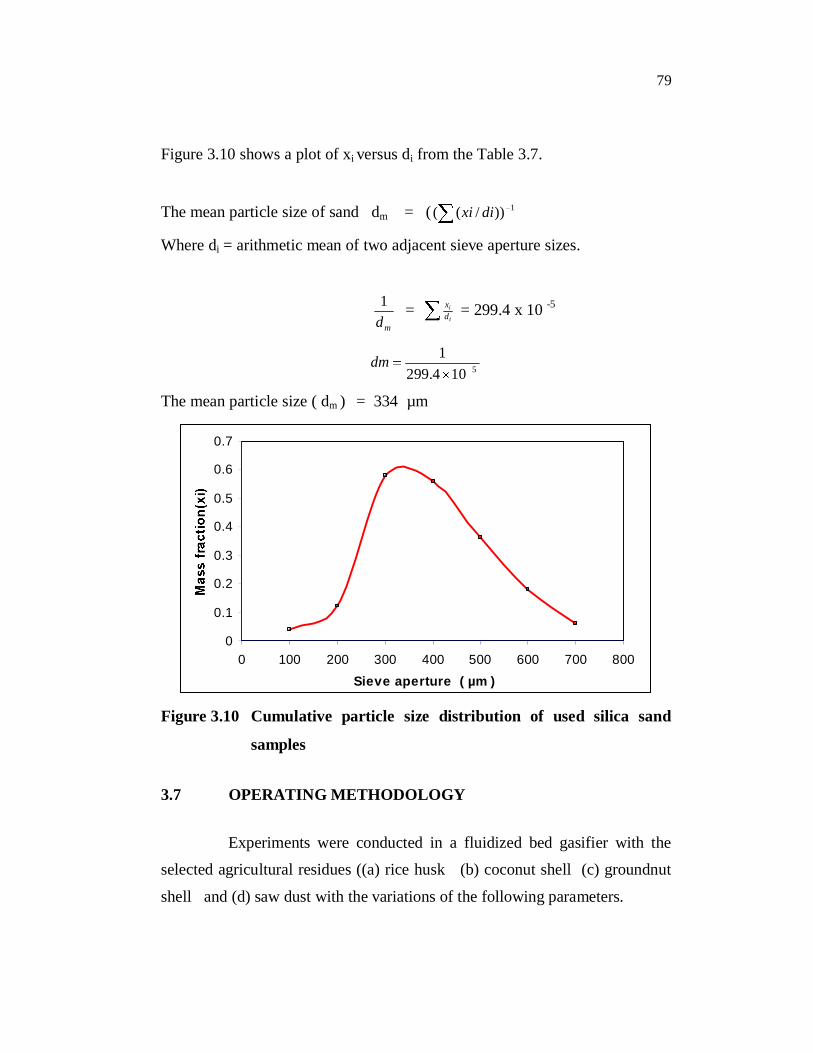
Figure 3.10 shows a plot of xi versus di from the Table 3.7.

The mean particle size of sand dm = ( 1))/(( dixi

Where di = arithmetic mean of two adjacent sieve aperture sizes.

md1 =

i

idx = 299.4 x 10 -5

5104.2991dm

The mean particle size ( dm ) = 334 µm

0

0.1

0.2

0.3

0.4

0.5

0.6

0.7

0 100 200 300 400 500 600 700 800Sieve aperture ( µm )

Figure 3.10 Cumulative particle size distribution of used silica sand

samples

3.7 OPERATING METHODOLOGY

Experiments were conducted in a fluidized bed gasifier with the

selected agricultural residues ((a) rice husk (b) coconut shell (c) groundnut

shell and (d) saw dust with the variations of the following parameters.

80

Bed temperature ranges from 650 to 900°C

Steam to Biomass ratio ranges from 0 to 1.0

Physical and chemical properties of samples in terms of

particle density, ash, oxygen and carbon content in the sample.

The experimental schedule has been designed in order to analyze

the individual effects of the main parameters governing the producer gas

quality (composition, production) and the gasification performance (gas yield,

energy content of the fuel gas), such as: a) varying the bed temperature in the

range from 650 ºC to 900 ºC; b) varying the steam to biomass ratio in the

range from 0 to 1. At the start of each experimental run, the agricultural

residue (Coconut Shell, Groundnut Shell, Rice husk and Sawdust) was added

to the hopper. In order to study the fluidization behaviour of the selected

material, it is loaded in to the bed and then fluidized vigorously to break down

any packing or interlocking of the particles. The air flow rate is gradually

decreased in steps and the pressure drop across the bed is recorded for each

air flow rate. In order to study the fluidization behaviour of the selected

biomass fuels, each fuel is first loaded in the bed. The air supply is increased

gradually to bring the bed of particles into fluization regime. Then the

velocity is gradually decreased, while recording the pressure drop across the

bed. In compare with other fuels, for rice husk high superficial velocities are

required to fluidize the rice husk particles because of their inter-particle

friction due to their rough abrasive surfaces. The minimum fluidized bed

velocity is found to be about 50 cm / s from its pressure drop curve.

To start the experiment test, the furnace heater was set at the

selected operating temperature. At the beginning of the experiment, the

reactor was charged with 3 kg of silica sand of mean diameter 0.334 mm as a

bed material, which helped in stable fluidization and better heat transfer.

81

After the bed temperature reached the desired level and became

remained steady, the samples were fed to the fluidized bed reactor and the

flow rate of biomass was controlled by a variable speed motor drive. The

supply of air was gradually reduced and the super heated steam at 200 ºC was

introduced at the side of the reactor. The bed was operated in fluidized

condition with air as fluidizing medium and steam as gasifying medium and

the test began. Five samples were taken at an interval of 3 minutes after the

test ran in a stable state. Normally each experiment was repeated two times

and the results were good agreement. The gas stream was passes through a

water scrubber followed by a dry filter. Grab samples of cool, clean and dry

gas were collected and analyzed in on line gas analyzer for the permanent

gases H2, CO, CO2 and CH4.

Experiments performed in the fluidized bed gasifier were carried

out in two groups for all the samples. In the first, to determine the effect of the

temperature (650 to 900 ºC) on the gas composition, gas yield, LHV, carbon

conversion efficiency at a constant fuel feed rate and equivalence ratio. The

second group of experiments was performed in order to determine the effect

of steam to biomass ratio (0 to 1.0) on the gas composition, gas yield, LHV,

carbon conversion efficiency. The biomass ow rate for the selected fuels rice

husk, coconut shell, groundnut shell and sawdust were varied from 1.5 to 6

kg/h, 4 to 18 kg/hr, 8 to 35 kg/h and 5 to 25 kg/h respectively.

Equilibrium modeling was carried out to predict the producer gas

composition under varying performance influencing parameters, viz.,

temperature, steam to biomass ratio. The results were compared with the

experimental output. Thermodynamic equilibrium composition prediction is

the important step in modeling the gasification process. Here the biomass is

represented as CHxOy. The biomass is reacted with steam and air to give

82

product gases viz. CO, CO2, H2 and CH4. The model assumes that the

principle reactions are at thermodynamic equilibrium. The model equations

containing three atom balances (C, O, and H) and three equilibrium relations

are solved for gas compositions.

3.8 DATA REDUCTION

The main performance characteristics evaluated from the measured

data were equivalence ratio, carbon conversion efficiency, heating value

(Lv et al 2004).

i) Equivalence ratio:

E.R. = Weight of oxygen( air ) / weight of drybiomassStoichiometricoxygen( air )weight of drybiomass

(3.1)

ii) Hot gas efficiency :

hot gas efficiency =

= 100//// 33

kgkJfuelofHHVhkgnconsumptioFuelmkJgasofHHVhmrateflowgasFuel (3.2)

iii) Cold gas efficiency :

cold gas efficiency =

= 100/

// 33

kgkJsystemtheinfedbiomasstheofLHVkgmproductiongasFuelmkJgasofLHV (3.3)

iv) Carbon conversion efficiency :

Carbon conversion = 4 2 12 10022 4

Gy(CO% CH % CO %). C%

(3.4)

where C% is the mass percentage of carbon in the feed obtained

from the ultimate analysis of the biomass.

v) Gas Yield:

Gy =3Product gas( Nm )

Dry biomass( kg ) (3.5)

83

vi) Dry product gas low heating value, LHV (kJ/ Nm3)

LHV = (30.0 CO + 25.7 H 2 + 85.4 CH4 + 151.3 Cn Hm) +

4 .2 kJ / Nm3 (3.6)

where CO, H2, etc. are the gas concentrations of the product gas.

vii) The HHV of the dry gas was determined from the following

equation (Xiao et al 2006):

HHV = (H2% 30.52 + CO% 30.18 + CH4% 95)

4.1868 (MJ/Nm3) (3.7)

where H2, CO and CH4 are the volumetric percentage in the fuel

gas.

3.9 MODELING

To model the gasification process in detail, knowledge of chemical

reaction kinetics is required which is not available in open literature.

Thermodynamic equilibrium composition prediction is the important step in

modeling the gasification process. Here the biomass is represented as CHxOy.

The biomass is reacted with steam and air to give product gases viz. CO, CO2,

H2 and CH4. The model assumes that the principle reactions are at

thermodynamic equilibrium. The model equations containing four atom

balances (C, O, H and N) and three equilibrium relations are solved for gas

compositions. The four types of biomasses are used for prediction of

equilibrium gas compositions The process of biomass gasification involves

three steps, which are: the initial devolatiliation or pyrolysis step which

produces volatile matter and a char residue, followed by secondary reactions

involving the volatile products and finally, the gasification reactions of the

remaining carbonaceous residue with steam and carbon dioxide. The biomass

84

devolatilization occurs instantaneously after its introduction to the reactor

resulting in volatiles and char.

Different types of models have been developed by Vamvuka et al

(1995), Ruggiero and manfrida (1999) for gasification systems - kinetic,

equilibrium and others. Unlike kinetic models that predict the progress and

product composition at different positions along a reactor, an equilibrium

model predicts the maximum achievable yield of a desired product from a

reacting system. It also provides a useful design aid in evaluating the limiting

possible behaviour of a complex reacting system which is difficult to

reproduce experimentally or in commercial operation.

At chemical equilibrium, a reacting system is at its most stable

composition, a condition achieved when the entropy of the system is

maximized, while its Gibbs free energy is minimized.

Smith and Missen (1982) described two approaches for equilibrium

modeling: stoichiometric and non-stoichiometric. The stoichiometric

approach requires a clearly defined reaction mechanism incorporating all

chemical reactions and species involved. In a non-stoichiometric formulation,

on the other hand, no particular reaction mechanism or species are involved in

the numerical solution. The only input needed to specify the feed is its

elemental composition, which can be readily obtained from ultimate analysis

data. This method is particularly suitable for problems with unclear reaction

mechanisms as well as feed streams like biomass, whose precise chemical

compositions are unknown. In the equilibrium model, the reactor is implicitly

considered to be zero-dimensional, i.e. neither spatial distribution nor change

of parameters with time is considered because all forward and reverse

reactions have reached chemical equilibrium. The molar inflow for any

individual element involved in the chemical reactions can then be written as

the sum of moles of that element in the various feed streams.

85

3.9.1 Assumptions

In view of this, a thermodynamic equilibrium model was used to

predict the gas composition. The basic assumptions of the present model

are:

Biomass is represented by the general formula CHxOy

The ideal gas laws are valid.

All reactions are at thermodynamic equilibrium.

The gasification products contain CO2, CO, H2, CH4, N2, H2O

Nitrogen present in both fuel and air is inert.

The pressure is atmospheric and constant in the char bed.

Ash is inert and is not involved in any reactions, either as a

chemical species or as a catalyst.

No gas is accumulated in the char bed.

There is no tar in the gasification zone.

To develop the model, the chemical formula of rice husk as a

biomass feedstock is defined as CH1.56O0.62. The global air-steam gasification

reaction can be written as follows (Koroneos and Lykidou 2011)

CHxOy + w H2O + m (O2 + 3.76N2 ) = x1H2 + x2CO + x3 CO2

+ x4 H2O + x5 CH4 + 3.76 m N2 (3.8)

where, x and y are the number of atoms of hydrogen and oxygen per number

of carbon in the biomass. The moisture content of the biomass is neglected

and the product quality depends on the x and y.

86

The above reaction represents an overall reaction but a number of

competing intermediate reactions take place during the process. These are,

1) Oxidation :

C + O2 CO2 H0r = - 393.8 kJ / mol (3.9)

2) Steam gasification :

C + H2O CO + H2 H0r = + 131.3 kJ / mol (3.10)

3) Boudouard reaction :

C + CO2 2 CO H0r = + 172.6 kJ / mol (3.11)

4) Methanation reaction :

C + 2H2 = CH4 H0r = - 74.9 kJ / mol (3.12)

5) Water gas-shift reaction :

CO + H2O = CO2 + H2 H0r = - 41.2 kJ / mol (3.13)

According to Von Fredersdorff and Elliot (1963), the three

reactions namely, Boudouard (equation 3.11), steam gasification (equation

3.10) and methanation (equation 3.12) are in equilibrium and the water gas

shift reaction (equation 3.13) is a combination of the Boudouard and steam

gasification reactions. Hence, the water gas shift and methanation reaction

could be considered to be in equilibrium. Oxidation reaction (equation 3.9) is

typically assumed to be very fast and goes to completion.

To find the five unknown species i.e. x1, x2, x3, x4 and x5 of the fuel

gas, five equations are required. Those equations are generated using mass

balance and equilibrium constant relationships.

87

3.9.2 Mass balance

Considering the global air-steam gasification reaction in equation

(3.8), the first three equations were formulated by balancing each chemical

element as shown in equation (3.14) to equation (3.16) (Ramirez et al 2007).

Taking atom balances on carbon, oxygen, hydrogen and nitrogen,

we obtain,

Carbon 1 = x2 + x3 + x5 (3.14)

Oxygen y + w + 2 m = x2 + 2 x3 + x4 (3.15)

Hydrogen x + 2 w = 2 x1 + 2 x4 + 4 x5 (3.16)

3.10 THERMODYNAMIC EQUILIBRIUM

Equilibrium is explained either by minimization of Gibb’s free

energy or using an equilibrium constant. To minimize the Gibb’s free energy,

constrained optimization methods are generally employed. Thus, to avoid

complicated mathematical theories associated with this Gibb’s free energy

approach, the present model in this study is based on the equilibrium constant

method, although it has been developed based on thermodynamic equilibrium.

From the Zainal et al (2001), the equilibrium constant K is a

function of temperature and can be written as,

0

eGln K

RT(3.17)

where, G0 is the Gibb’s free energy (kJ/mol), T is the temperature in K and R

is the universal gas constant in consistent units.

88

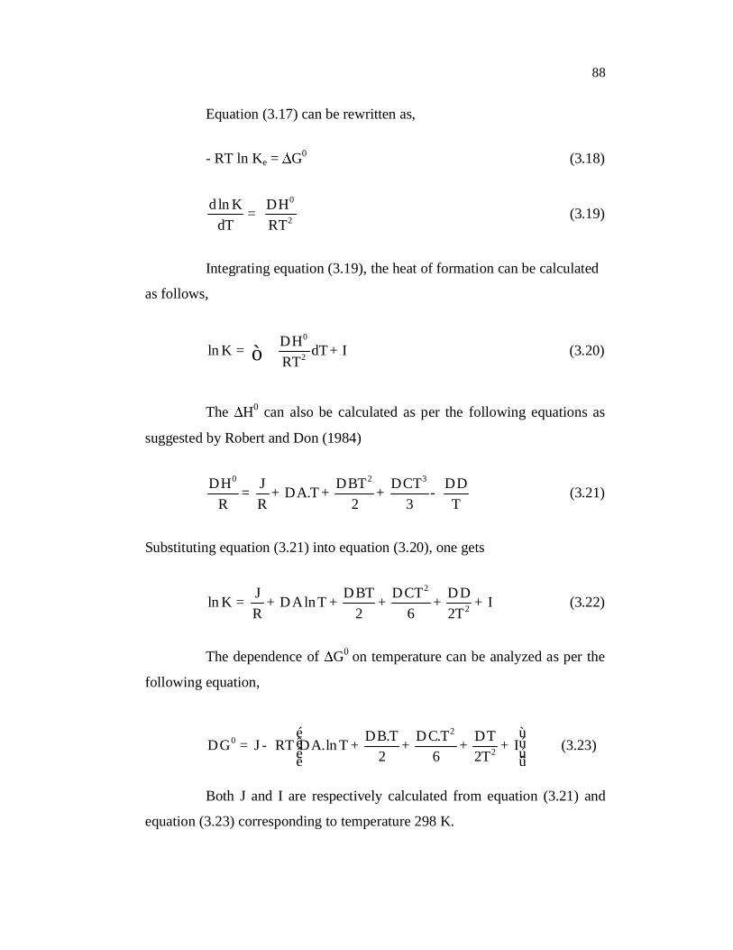
Equation (3.17) can be rewritten as,

- RT ln Ke = G0 (3.18)

0

2d ln K H

dT RTD= (3.19)

Integrating equation (3.19), the heat of formation can be calculated

as follows,

0

2Hln K dT I

RTD= +ò (3.20)

The H0 can also be calculated as per the following equations as

suggested by Robert and Don (1984)

0 2 3H J BT CT DA.TR R 2 3 T

D D D D= + D + + - (3.21)

Substituting equation (3.21) into equation (3.20), one gets

2

2J BT CT Dln K Aln T IR 2 6 2T

D D D= + D + + + + (3.22)

The dependence of G0 on temperature can be analyzed as per the

following equation,

20

2B.T C.T TG J RT A.ln T I2 6 2T

é ùD D Dê úD = - D + + + +ê úë û(3.23)

Both J and I are respectively calculated from equation (3.21) and

equation (3.23) corresponding to temperature 298 K.

89

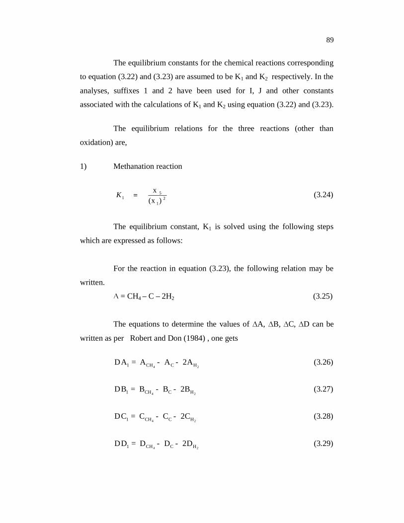
The equilibrium constants for the chemical reactions corresponding

to equation (3.22) and (3.23) are assumed to be K1 and K2 respectively. In the

analyses, suffixes 1 and 2 have been used for I, J and other constants

associated with the calculations of K1 and K2 using equation (3.22) and (3.23).

The equilibrium relations for the three reactions (other than

oxidation) are,

1) Methanation reaction

)x(x

21

51K (3.24)

The equilibrium constant, K1 is solved using the following steps

which are expressed as follows:

For the reaction in equation (3.23), the following relation may be

written.

= CH4 – C – 2H2 (3.25)

The equations to determine the values of A, B, C, D can be

written as per Robert and Don (1984) , one gets

4 21 CH C HA A A 2AD = - - (3.26)

4 21 CH C HB B B 2BD = - - (3.27)

4 21 CH C HC C C 2CD = - - (3.28)

4 21 CH C HD D D 2DD = - - (3.29)

90

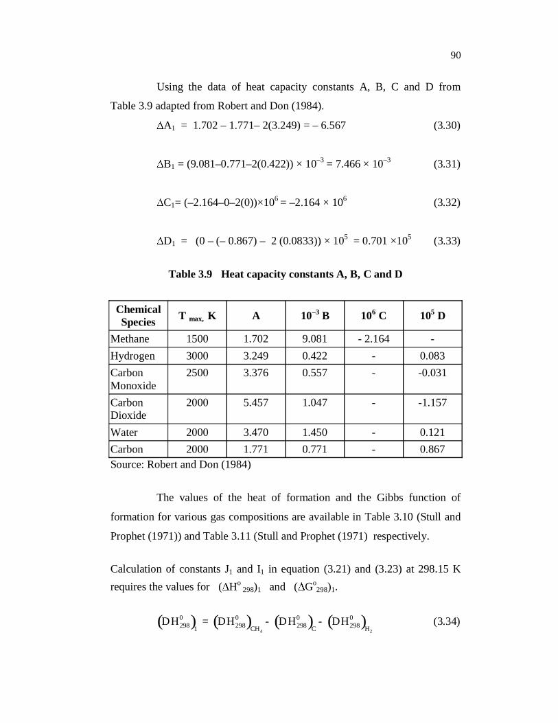
Using the data of heat capacity constants A, B, C and D from

Table 3.9 adapted from Robert and Don (1984).

A1 = 1.702 – 1.771– 2(3.249) = – 6.567 (3.30)

B1 = (9.081–0.771–2(0.422)) × 10–3 = 7.466 × 10–3 (3.31)

C1= (–2.164–0–2(0))×106 = –2.164 × 106 (3.32)

D1 = (0 – (– 0.867) – 2 (0.0833)) × 105 = 0.701 ×105 (3.33)

Table 3.9 Heat capacity constants A, B, C and D

ChemicalSpecies T max, K A 10–3 B 106 C 105 D

Methane 1500 1.702 9.081 - 2.164 -Hydrogen 3000 3.249 0.422 - 0.083CarbonMonoxide

2500 3.376 0.557 - -0.031

CarbonDioxide

2000 5.457 1.047 - -1.157

Water 2000 3.470 1.450 - 0.121Carbon 2000 1.771 0.771 - 0.867Source: Robert and Don (1984)

The values of the heat of formation and the Gibbs function of

formation for various gas compositions are available in Table 3.10 (Stull and

Prophet (1971)) and Table 3.11 (Stull and Prophet (1971) respectively.

Calculation of constants J1 and I1 in equation (3.21) and (3.23) at 298.15 Krequires the values for ( Ho

298)1 and ( Go298)1.

( ) ( ) ( ) ( )4 2

0 0 0 0298 298 298 2981 CH C H

H H H HD = D - D - D (3.34)

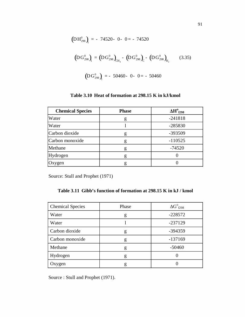
91

( )0298 1

H 74520 0 0 74520D = - - - = -

( ) ( ) ( ) ( )4 2

0 0 0 0298 298 298 2981 CH C H

G G G GD = D - D - D (3.35)

( )0298 1

G 50460 0 0 50460D = - - - = -

Table 3.10 Heat of formation at 298.15 K in kJ/kmol

Chemical Species Phase Hof298

Water g -241818Water l -285830Carbon dioxide g -393509Carbon monoxide g -110525Methane g -74520Hydrogen g 0Oxygen g 0

Source: Stull and Prophet (1971)

Table 3.11 Gibb’s function of formation at 298.15 K in kJ / kmol

Chemical Species Phase Gof298

Water g -228572

Water l -237129

Carbon dioxide g -394359

Carbon monoxide g -137169

Methane g -50460

Hydrogen g 0

Oxygen g 0

Source : Stull and Prophet (1971).

92

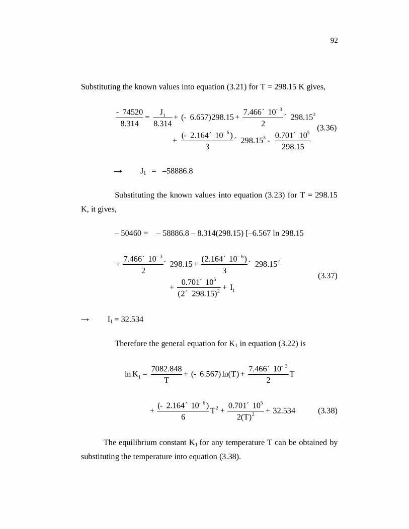
Substituting the known values into equation (3.21) for T = 298.15 K gives,

321

6 53

74520 J 7.466 10( 6.657)298.15 298.158.314 8.314 2

( 2.164 10 ) 0.701 10298.153 298.15

-

-

- ´= + - + ´

- ´ ´+ ´ -(3.36)

J1 = –58886.8

Substituting the known values into equation (3.23) for T = 298.15

K, it gives,

– 50460 = – 58886.8 – 8.314(298.15) [–6.567 ln 298.15

3 62

5

12

7.466 10 (2.164 10 )298.15 298.152 3

0.701 10 I(2 298.15)

- -´ ´+ ´ + ´

´+ +´

(3.37)

I1 = 32.534

Therefore the general equation for K1 in equation (3.22) is

3

17082.848 7.466 10ln K ( 6.567) ln(T) T

T 2

-´= + - +

6 52

2( 2.164 10 ) 0.701 10T 32.534

6 2(T)

-- ´ ´+ + + (3.38)

The equilibrium constant K1 for any temperature T can be obtained by

substituting the temperature into equation (3.38).

93

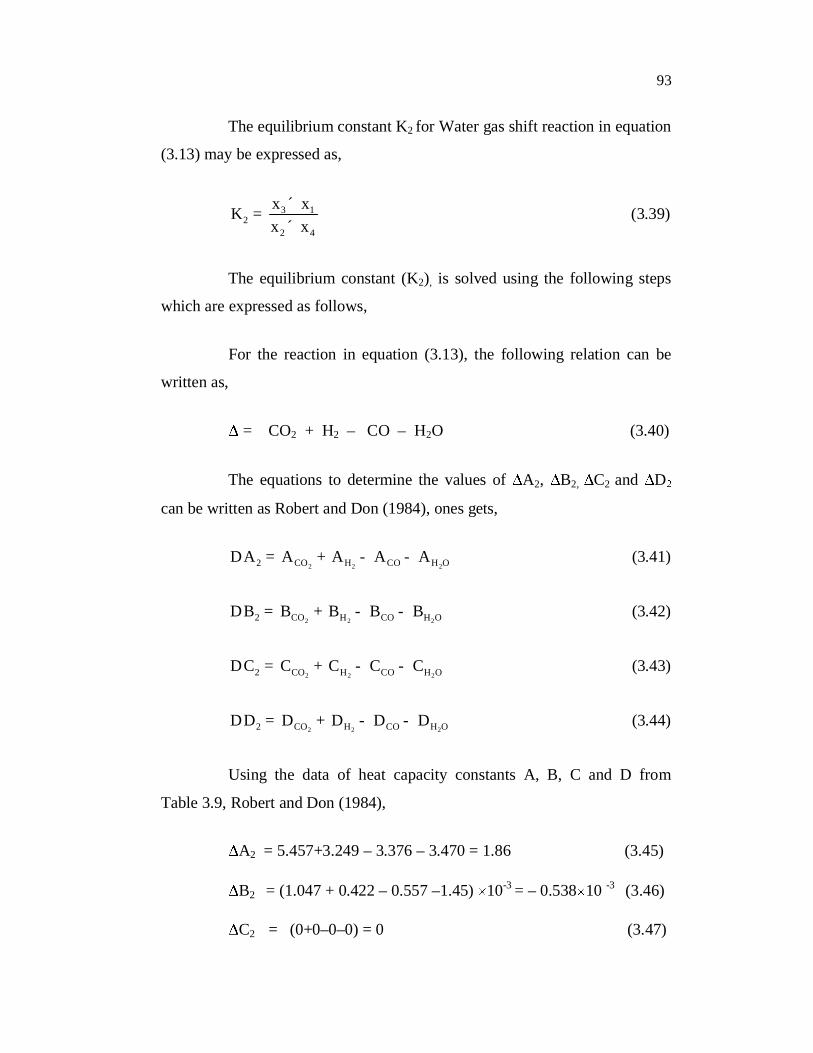
The equilibrium constant K2 for Water gas shift reaction in equation

(3.13) may be expressed as,

3 12

2 4

x xKx x

´=´

(3.39)

The equilibrium constant (K2), is solved using the following steps

which are expressed as follows,

For the reaction in equation (3.13), the following relation can be

written as,

= CO2 + H2 – CO – H2O (3.40)

The equations to determine the values of A2, B2, C2 and D

can be written as Robert and Don (1984), ones gets,

2 2 22 CO H CO H OA A A A AD = + - - (3.41)

2 2 22 CO H CO H OB B B B BD = + - - (3.42)

2 2 22 CO H CO H OC C C C CD = + - - (3.43)

2 2 22 CO H CO H OD D D D DD = + - - (3.44)

Using the data of heat capacity constants A, B, C and D from

Table 3.9, Robert and Don (1984),

A2 = 5.457+3.249 – 3.376 – 3.470 = 1.86 (3.45)

B2 = (1.047 + 0.422 – 0.557 –1.45) 10-3 = – 0.538 10 -3 (3.46)

C2 = (0+0–0–0) = 0 (3.47)

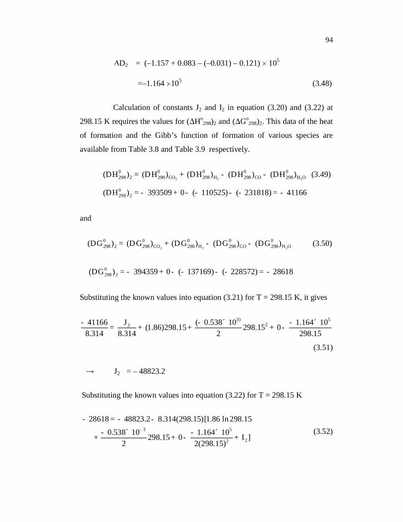
94

D2 = (–1.157 + 0.083 – (–0.031) – 0.121) 105

=–1.164 105 (3.48)

Calculation of constants J2 and I2 in equation (3.20) and (3.22) at

298.15 K requires the values for ( Ho298)2 and ( Go

298)2. This data of the heat

of formation and the Gibb’s function of formation of various species are

available from Table 3.8 and Table 3.9 respectively.

2 2 2

0 0 0 0 0298 2 298 CO 298 H 298 CO 298 H O( H ) ( H ) ( H ) ( H ) ( H )D = D + D - D - D (3.49)

0298 2( H ) 393509 0 ( 110525) ( 231818) 41166D = - + - - - - = -

and

2 2 2

0 0 0 0 0298 2 298 CO 298 H 298 CO 298 H O( G ) ( G ) ( G ) ( G ) ( G )D = D + D - D - D (3.50)

0298 2( G ) 394359 0 ( 137169) ( 228572) 28618D = - + - - - - = -

Substituting the known values into equation (3.21) for T = 298.15 K, it gives

3) 52241166 J ( 0.538 10 1.164 10(1.86)298.15 298.15 0

8.314 8.314 2 298.15- - ´ - ´= + + + -

(3.51)

J2 = – 48823.2

Substituting the known values into equation (3.22) for T = 298.15 K

3 5

22

28618 48823.2 8.314(298.15)[1.86 ln 298.15

0.538 10 1.164 10298.15 0 I ]2 2(298.15)

-

- = - -

- ´ - ´+ + - + (3.52)

95

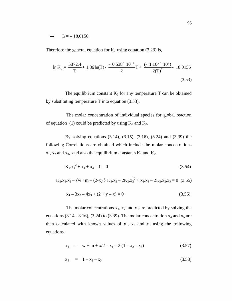
I2 = – 18.0156.

Therefore the general equation for K2 using equation (3.23) is,

3 5

2 25872.4 0.538 10 ( 1.164 10 )ln K 1.86ln(T) T 18.0156

T 2 2(T)

-- ´ - ´= + - + -

(3.53)

The equilibrium constant K2 for any temperature T can be obtained

by substituting temperature T into equation (3.53).

The molar concentration of individual species for global reaction

of equation (1) could be predicted by using K1 and K2.

By solving equations (3.14), (3.15), (3.16), (3.24) and (3.39) the

following Correlations are obtained which include the molar concentrations

x1, x2 and x3, and also the equilibrium constants K1 and K2

K1.x12 + x2 + x3 – 1 = 0 (3.54)

K2.x1.x2 – {w +m – (2-x) } K2.x2 – 2K2.x22 + x1.x3 – 2K2.x2.x3 = 0 (3.55)

x1 – 3x2 – 4x3 + (2 + y – x) = 0 (3.56)

The molar concentrations x1, x2 and x3 are predicted by solving the

equations (3.14 - 3.16), (3.24) to (3.39). The molar concentration x4 and x5 are

then calculated with known values of x1, x2 and x3 using the following

equations.

x4 = w + m + x/2 – x1 – 2 (1 – x2 – x3) (3.57)

x5 = 1 – x2 – x3 (3.58)

96

where, x and y are the number of atoms of hydrogen and oxygen per number

of carbon in the biomass. The moisture content of the biomass is neglected

and the product quality depends on the x and y.

3.11 ENERGY BALANCE

Energy balance equation of reactants and products of global steam

gasification reaction in equation (3.8) is shown in the following.

22)(22... 1 Hf

oinOHOHf

o CpTHxQHmHwH HlRH

22.. 32 COf

oCOf

o CpTHxCpTHx COCO

+4422 .. 54 CHf

oOHvapf

o CpTHxCpTHx CHOH (3.59)

The heat balance equation (3.59) contains a term Qin which stands

for the external heat addition required for endothermic reactions to occur.

2 2

22 22

42 42

( ) ( )

1 2 3

4 5

.( ) . . )

( . ) ( . ) ( . )

( . ) ( . )

RH

H H CO CO CO CO

H H O CH CHO

O Of H O l vap H O g fs P Fs in

O O Of P f P f P

O Of P f P

H w H H m H T C Q

x H T C x H T C x H T C

x H T C x H T C

Since 02H

fOH then the above equation may be written as,

=> inFSFSOfHo

vaplOHo

fo QCpTHmHfHwH gRH 22

.. )(

222... 321 COf

oCOf

oH CpTHxCpTHxCpTx COCO

4422.. 54 CHf

oOHf

o CpTHxCpTHx CHOH (3.61)

inOHOHfo QdHmdHwH

FSRHRH 22..

4222..... 54321 CHgOHCOCOH dHxdHxdHxdHxdHx (3.62)

inOHOHfo QdHmdHwH

FSRHRH 22..

(3.60)

97

42

22

.1.222

...

32321

321

CHgOH

COCOH

dHxxdHxxxxmw

dHxdHxdHx(3.63)

inOHOHfo QdHmdHwH

FSRHRH 22..

42422

4222

.22

.2

3

21

CHgOHCHgOHCO

CHgOHCOgOHH

dHdHxmwdHdHdHx

dHdHdHxdHdHx

(3.64)

gOHfo

CHOHgOH

RHOHgOHCHOHCO

CHgOHCOgOHHin

dHxHdHdHdHm

dHdHwdHdHdHx

dHdHdHxdHdHxQ

RHFS 2

3

21

2.

.2.

...

422

22422

42222

(3.65)

Now the expression of Qin may be stated as follows,

Qin = a 1.x1 + a 2.x2 + a 3.x3 + a 4.w + a5.m + a 6 (3.66)

where,

gOHfo

CH

FSOHgOH

RHOHgOH

CHOHCO

CHOHCO

gOHH

dHxHdHa

dHdHa

dHdHa

dHdHdHa

dHdHdHa

dHdHa

RH 24

22

22

422

42

22

2

2

2

6

5

4

3

2

1

(3.67)

and

98

222. Hf

oH CpTHdH H

2121

2 22

222.4

3.

TTD

TTTC

TBATdH Hm

HmHHH (3.68)

COfo

CO CpTHdH CO .

2121

2.43

.TT

DTTT

CTBATHdH CO

mCO

mCOCOfo

CO CO (3.69)

222. COf

oCO CpTHdH CO

2121

2 22

2222.4

3.

TTD

TTTC

TBATHdH COm

COmCOCOf

oCO CO (3.70)

444. CHf

oCH CpTHdH CH

2121

24 4

4444.4

3.

TTD

TTTC

TBATHdH CHm

CHmCHCHf

oCH CH (3.71)

vapfo

OH HHdH lOHRH 22 (3.72)

FSOHFSOHfo

FSOH CpTHdH g 222.

FS

gOHFSFSm

gOH

FSmgOHgOH

FSgOHfo

FSOH

TTD

TTTC

TBATHdH

1

21

243

..

2

22

22 (3.73)

gOHFSOHfo

gOH CpTHdH g 222.

99

21

221

243

..

2

22

22

TTD

TTmTC

TBATHdH gOHgOH

mgOHgOH

OHfo

gOH g (3.74)

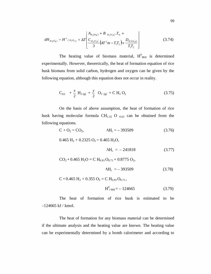
The heating value of biomass material, H0fRH is determined

experimentally. However, theoretically, the heat of formation equation of rice

husk biomass from solid carbon, hydrogen and oxygen can be given by the

following equation, although this equation does not occur in reality.

C(s) + 2x H2 (g) +

2y O2 (g) = C Hx Oy (3.75)

On the basis of above assumption, the heat of formation of rice

husk having molecular formula CH1.55 O 0.63 can be obtained from the

following equations.

C + O2 = CO2, Hc = – 393509 (3.76)

0.465 H2 + 0.2325 O2 = 0.465 H2O,

Hc = – 241818 (3.77)

CO2 + 0.465 H2O = C H0.93 O0.71 + 0.8775 O2,

Hc = – 393509 (3.78)

C + 0.465 H2 + 0.355 O2 = C H0.93 O0.71 ,

H0f RH = – 124665 (3.79)

The heat of formation of rice husk is estimated to be

–124665 kJ / kmol.

The heat of formation for any biomass material can be determined

if the ultimate analysis and the heating value are known. The heating value

can be experimentally determined by a bomb calorimeter and according to

100

Reed (1985), the heat of formation in MJ/kg of any biomass material can be

calculated with reasonably good accuracy from the following equation

Hc = 0.2326(146.58 C + 56.878 H – 51.53 O – 6.58 A + 29.45) (3.80)

where C, H, O and A are the mass fractions of carbon, hydrogen, oxygen and

ash respectively in the dry biomass which are obtained from the ultimate

analyses for various biomass fuels. The dependence of specific heat on

temperature is given by various empirical equations and most simplified

version is adapted from Robert and Don (1984) is,

Cp am = R [ A+ B Tam+C(4T2am – T1T2) / 3 + D / (T1T2)] (3.81)

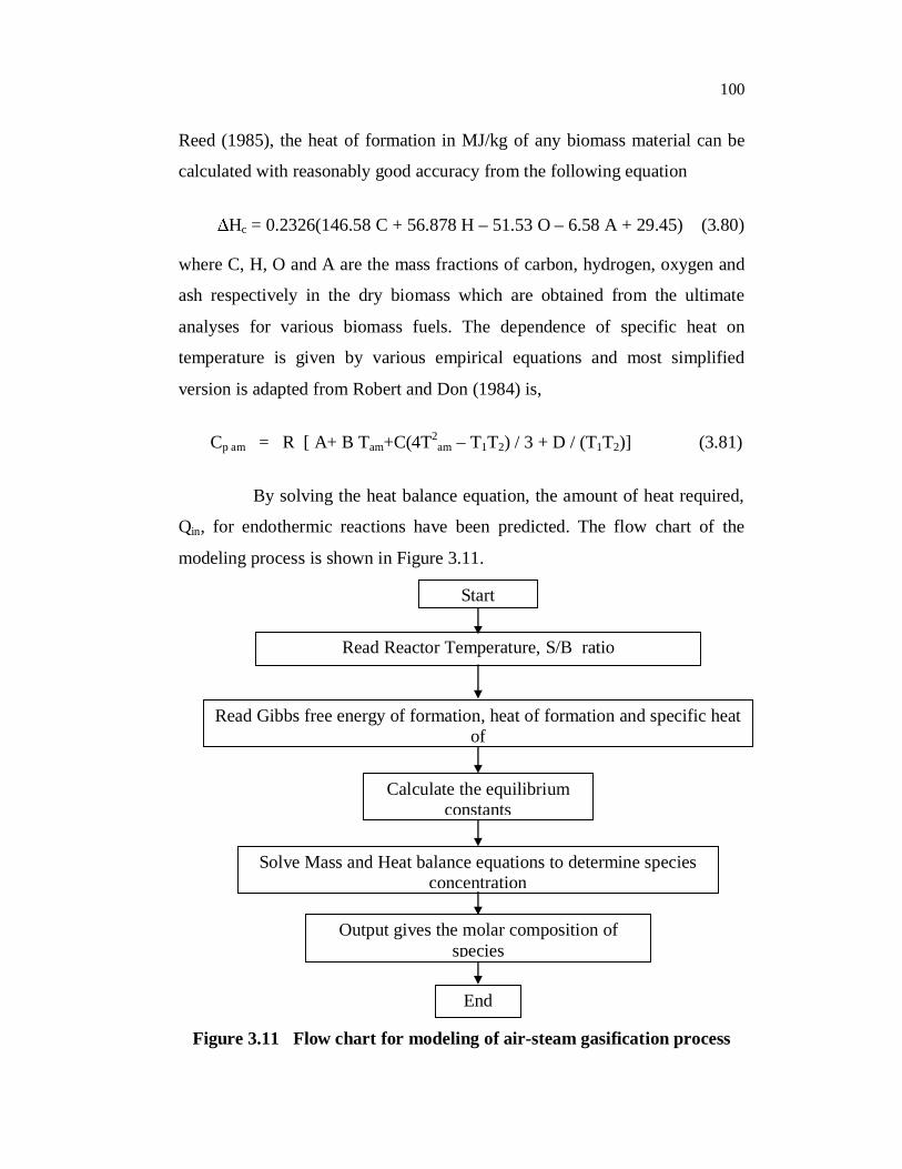
By solving the heat balance equation, the amount of heat required,

Qin, for endothermic reactions have been predicted. The flow chart of the

modeling process is shown in Figure 3.11.

Figure 3.11 Flow chart for modeling of air-steam gasification process

Start

Read Reactor Temperature, S/B ratio

Read Gibbs free energy of formation, heat of formation and specific heatof

Calculate the equilibriumconstants

Solve Mass and Heat balance equations to determine speciesconcentration

Output gives the molar composition ofspecies

End