Chapter 3 : Dynamic Game Theory. In the previous chapter we focused on static games. However for many important economic applications we need to think of the game as being played over a number of time periods, making it dynamic. A game can be dynamic for two reasons. First, the interaction between players may itself be inherently dynamic. In this situation players are able to observe the actions of other players before deciding upon their optimal response. In contrast static games are ones where we can think of players making their moves simultaneously. Second, a game is dynamic if a one-off game is repeated a number of times, and players observe the outcome of previous games before playing later games. In section 3.1 we consider one-off dynamic games, and in section 3.2 we analyse repeated games.

3.1. Dynamic One-Off Games. An essential feature of all dynamic games is that some of the players can condition their optimal actions on what other players have done in the past. This greatly enhances the strategies available to such players, in that these are no longer equivalent to their possible actions. To illustrate this we examine the following two period dynamic entry game, which is a modified version of the static game used in Exercise 2.4. There are two firms (A and B) that are considering whether or not to enter a new market. Unfortunately the market is only big enough to support one of the two firms. If both firms enter the market then they will both make a loss of £10 million. If only one firm enters the market, that firm will earn a profit of £50 million, and the other firm will just break even. To make this game dynamic we assume that firm B observes whether firm A has entered the market before it decides what to do. This game can be represented by the extensive form diagram shown in Figure 3.1.

Firm A

Firm B

Firm B

(- £10m , - £10m)

(£50m , 0)

(0 , £50m)

(0 , 0)

Enter

Stay

Enter

Stay

Stay

Out

Out

Out

Enter

Figure 3.1. The Dynamic Entry Game in Extensive Form. In time period 1 firm A makes its decision. This is observed by firm B which decides to enter or stay out of the market in period 2. In this extensive form game firm B’s decision nodes are separate information sets. (If they were in the same information set they would be connected by a dashed line.) This means that firm B observes firm A’s action before making its own decision. If the two firms were to make their moves simultaneously then firm B would have only two strategies. These would be to either enter or stay out of the market. However because firm B initially observes firm A’s decision it can make its decision conditional upon what firm A does. As firm A has two possible actions, and so does firm B, this means that firm B has four (2 x 2) strategies. We can list these as

Always enter the market whatever firm A does. Always stay out of the market whatever firm A does. Do the same as firm A. Do the opposite of firm A.

Recognizing that firm B now has these four strategies we can represent the above game in normal form. This is shown in Figure 3.2. Having converted the extensive form game into a normal form game we can apply the two stage method for finding pure strategy Nash equilibria, as explained in the previous chapter. First, we identify what each player’s optimal strategy is in response to what the other players might do. This involves working through each player in turn and determining their optimal strategies. This is illustrated in the normal form game by underlining the relevant payoff. Second, a Nash equilibrium is identified when all players are playing their optimal strategies simultaneously. Firm B Firm A

Figure 3.2. The Dynamic Entry Game in Normal Form. As shown in Figure 3.2 this dynamic entry game has three pure strategy Nash equilibria. In these three situations each firm is acting rationally given its belief about what the other firm might do. Both firms are maximizing their profits dependent upon what they believe the other firm’s strategy is. One way to understand these possible outcomes is to think of firm B making various threats or promises, and firm A acting accordingly. We can therefore interpret the three Nash equilibria as follows: 1. Firm B threatens to always enter the market irrespective of what firm A does.

If firm A believes this threat it will stay out of the market. 2. Firm B promises to always stay out of the market irrespective of what firm A

does. If firm A believes this promise it will certainly enter the market. 3. Firm B promises to always do the opposite of what firm A does. If firm A

believes this promise it will again enter the market. In the first two Nash equilibria firm B’s actions are not conditional on what the other firm does. In the third Nash equilibrium firm B does adopt a conditional strategy. A conditional strategy is where one player conditions their actions upon the actions of at least one other player in the game. This concept is particularly important in repeated games, and is considered in more detail in the next section. In each of the equilibria firm A is acting rationally in accordance with its beliefs. However this analysis does not consider which of its beliefs are themselves rational. This raises the interesting question “Could firm A not dismiss some of firm B’s threats or promises as mere bluff ?” This raises the important issue of credibility. The concept of credibility comes down to the question “Is a threat or promise believable ?” In game theory a threat or promise is only credible if it is in that player’s interest to carry it out at the appropriate time. In this sense some of firm B’s statements are not credible. For example, firm B may threaten to always enter the market irrespective of what firm A does, but this is not credible. It is not credible because if firm A enters the market then it is in firm B’s interest to stay out. Similarly the promise to always stay out of the market is not credible because if firm A does not enter then it is in firm B’s interest to do so. Assuming that player’s are rational,

ALWAYS ENTER

ALWAYS

STAY OUT

SAME AS FIRM A

OPPOSITE OF FIRM A

ENTER

- £10m -

£10m

£50m

0

- £10m - £10m

£50m

0

STAY OUT

0

£50m

0 0

0 0

0

£50m

and that this is common knowledge, it seems reasonable to suppose that player’s only believe credible statements. This implies that incredible statements will have no effect on other players behaviour. These ideas are incorporated into an alternative equilibrium concept to Nash equilibrium (or a refinement of it) called subgame perfect Nash equilibrium.

a. Subgame Perfect Nash Equilibrium. In many dynamic games there are multiple Nash equilibria. Often, however, these equilibria involve incredible threats or promises that are not in the interests of the players making them to carry out. The concept of subgame perfect Nash equilibrium rules out these situations by saying that a reasonable solution to a game cannot involve players believing and acting upon incredible threats or promises. More formally a subgame perfect Nash equilibrium requires that the predicted solution to a game be a Nash equilibrium in every subgame. A subgame, in turn, is defined as a smaller part of the whole game starting from any one node and continuing to the end of the entire game, with the qualification that no information set is subdivided. A subgame is therefore a game in its own right that may be played in the future, and is a relevant part of the overall game. By requiring that a solution to a dynamic game must be a Nash equilibrium in every subgame amounts to saying that each player must act in their own self interest in every period of the game. This means that incredible threats or promises will not be believed or acted upon. To see how this equilibrium concept is applied, we continue to examine the dynamic entry game discussed above. From the extensive form of this game, given in Figure 3.1, we can observe that there are two subgames, one starting from each of firm B’s decision nodes. For the predicted solution to be a subgame perfect Nash equilibrium it must comprise a Nash equilibrium in each of these subgames. We now consider each of the Nash equilibria identified for the entire game to see which, if any, are also a subgame perfect Nash equilibrium. 1. In the first Nash equilibrium firm B threatens to always enter the market irrespective of what firm A does. This strategy is, however, only a Nash equilibrium for one of the two subgames. It is optimal in the subgame beginning after firm A has stayed out but not in the one where firm A has entered. If firm A enters the market it is not in firm B’s interest to carry out the threat and so it will not enter. This threat is not credible and so should not be believed by firm A. This Nash equilibrium is not subgame perfect. 2. In the second Nash equilibrium firm B promises to always stay out of the market irrespective of what firm A does. Again this is only a Nash equilibrium for one of the two subgames. It is optimal in the subgame beginning after firm A has entered but not in the one when firm A has stayed out . If firm A stays out of the market, it is not in the interest of firm B to keep its promise, and so it will enter. This promise is not credible, and so should not be believed by firm A. Once more this Nash equilibrium is not subgame perfect. 3. The third Nash equilibrium is characterized by firm B promising to do the opposite of whatever firm A does. This is a Nash equilibrium for both subgames. If firm A enters it is optimal for firm B to stay out, and if firm A stays out it is optimal for firm B to enter. This is a credible promise because it is always in firm B’s interest to carry it out at the appropriate time in the future. This promise is therefore believable, and with this belief it is rational for firm A to enter the market. The only subgame perfect Nash equilibrium for this game is that firm A will enter and firm B will stay out. This seems entirely reasonable given that firm A has the ability to enter the market first. Once firm B observes this decision it will not want to enter the market, and so firm A maintains its monopoly position. The way we solved this dynamic game has been rather time consuming. This was done so that the concept of subgame perfection may be better understood. Fortunately there is often a quicker way of finding the subgame perfect Nash equilibrium of a dynamic game. This is by using the principle of backward induction.

b. Backward Induction. Backward induction is the principle of iterated strict dominance applied to dynamic games in extensive form. However, this principle involves ruling out the actions, rather than strategies, that players would not play because other actions give higher payoffs. In applying this principle to dynamic games we start with the last period first and work backwards through successive nodes until we reach the beginning of the game. Assuming perfect and complete information, and that no player is indifferent between two possible actions at any point in the

game, then this method will give a unique prediction which is the subgame perfect Nash equilibrium. Once more this principle is illustrated using the dynamic entry game examined above. The extensive form for this game is reproduced in Figure 3.3.

Firm A

Firm B

Firm B

(- £10m , - £10m)

(£50m , 0)

(0 , £50m)

(0 , 0)

Enter

Stay

Enter

Stay

Stay

Out

Out

Out

Enter

Figure 3.3. The Dynamic Entry Game and Backward Induction. Starting with the last period of the game first we have two nodes. At each of these nodes firm B decides whether or not to enter the market based on what firm A has already done. At the first node firm A has already entered and so firm B will either make a loss of £10m if it enters, or break even if it stays out. In this situation firm B will stay out, and so we can rule out the possibility of both firms entering. This is shown by crossing out the corresponding payoff vector (- £10m , - £10m). At the second node firm A has not entered the market, and so firm B will earn either £50m if it enters or nothing if it stays out. In this situation firm B will enter the market, and we can rule out the possibility of both firms staying out. Once more we cross out the corresponding payoff vector (0 , 0). We can now move back to the preceding nodes, which in this game is the initial node. Here firm A decides whether or not to enter. However if firm A assumes that firm B is rational then it knows the game will never reach the previously excluded strategies and payoffs. Firm A can reason therefore that it will either receive £50m if it enters or nothing if it stays out. Given this reasoning we can rule out the possibility that firm A will stay out of the market, and so cross out the corresponding payoff vector (0 , £50m). This leaves only one payoff vector remaining, corresponding to firm A entering the market and firm B staying out. This, as shown before, is the subgame perfect Nash equilibrium.

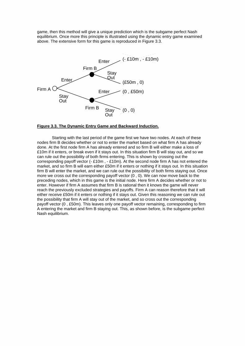
Exercise 3.1. Using the principle of backward induction find the subgame perfect Nash equilibrium for the following three player extensive form game. State all the assumptions you make.

1.

2.

2. 3.

(2 , 4 , 6)

(3 , 8 , 1)

(4 , 4 , 4) (10 , 1 , 7)

(6 , 8 , 9)

(3 , 1 , 2)

up

down

up

middle

down

up

down

up

down

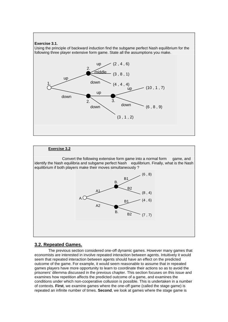
Exercise 3.2

Convert the following extensive form game into a normal form game, and identify the Nash equilibria and subgame perfect Nash equilibrium. Finally, what is the Nash equilibrium if both players make their moves simultaneously ?

A.

A1

A2

B.

B.

B1

B2

B1

B2

(6 , 8)

(8 , 4)

(4 , 6)

(7 , 7)

3.2. Repeated Games. The previous section considered one-off dynamic games. However many games that economists are interested in involve repeated interaction between agents. Intuitively it would seem that repeated interaction between agents should have an effect on the predicted outcome of the game. For example, it would seem reasonable to assume that in repeated games players have more opportunity to learn to coordinate their actions so as to avoid the prisoners’ dilemma discussed in the previous chapter. This section focuses on this issue and examines how repetition affects the predicted outcome of a game, and examines the conditions under which non-cooperative collusion is possible. This is undertaken in a number of contexts. First, we examine games where the one-off game (called the stage game) is repeated an infinite number of times. Second, we look at games where the stage game is

repeated only a finite number of times and where the one-off game has a unique Nash equilibrium. In this context we discuss the so called “paradox of backward induction”. This paradox is that while coordination may be possible in infinitely repeated games it is not possible in certain situations with finitely repeated games. This is true no matter how large the number of repetitions. Finally, we examine ways in which this paradox of backward induction may be avoided.

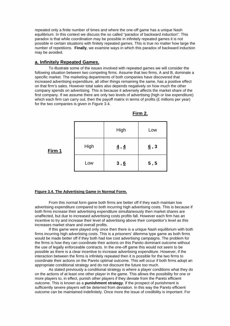
a. Infinitely Repeated Games. To illustrate some of the issues involved with repeated games we will consider the following situation between two competing firms. Assume that two firms, A and B, dominate a specific market. The marketing departments of both companies have discovered that increased advertising expenditure, all other things remaining the same, has a positive effect on that firm’s sales. However total sales also depends negatively on how much the other company spends on advertising. This is because it adversely affects the market share of the first company. If we assume there are only two levels of advertising (high or low expenditure) which each firm can carry out, then the payoff matrix in terms of profits (£ millions per year) for the two companies is given in Figure 3.4. Firm 1

Firm 2.

High

Low

High

4 , 4

6 , 3

Low

3 , 6

5 , 5

Figure 3.4. The Advertising Game in Normal Form. From this normal form game both firms are better off if they each maintain low advertising expenditure compared to both incurring high advertising costs. This is because if both firms increase their advertising expenditure simultaneously then market shares are unaffected, but due to increased advertising costs profits fall. However each firm has an incentive to try and increase their level of advertising above their competitor’s level as this increases market share and overall profits. If this game were played only once then there is a unique Nash equilibrium with both firms incurring high advertising costs. This is a prisoners’ dilemma type game as both firms would be made better off if they both had low cost advertising campaigns. The problem for the firms is how they can coordinate their actions on this Pareto dominant outcome without the use of legally enforceable contracts. In the one-off game this would not seem to be possible as there is a clear incentive to increase advertising expenditure. However, if the interaction between the firms is infinitely repeated then it is possible for the two firms to coordinate their actions on the Pareto optimal outcome. This will occur if both firms adopt an appropriate conditional strategy and do not discount the future too much. As stated previously a conditional strategy is where a player conditions what they do on the actions of at least one other player in the game. This allows the possibility for one or more players to, in effect, punish other players if they deviate from the Pareto efficient outcome. This is known as a punishment strategy. If the prospect of punishment is sufficiently severe players will be deterred from deviation. In this way the Pareto efficient outcome can be maintained indefinitely. Once more the issue of credibility is important. For

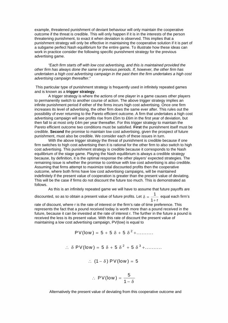
example, threatened punishment of deviant behaviour will only maintain the cooperative outcome if the threat is credible. This will only happen if it is in the interests of the person threatening punishment, to exact it when deviation is observed. This implies that a punishment strategy will only be effective in maintaining the cooperative solution if it is part of a subgame perfect Nash equilibrium for the entire game. To illustrate how these ideas can work in practice consider the following specific punishment strategy for the previous advertising game. “Each firm starts off with low cost advertising, and this is maintained provided the other firm has always done the same in previous periods. If, however, the other firm has undertaken a high cost advertising campaign in the past then the firm undertakes a high cost advertising campaign thereafter.” This particular type of punishment strategy is frequently used in infinitely repeated games and is known as a trigger strategy. A trigger strategy is where the actions of one player in a game causes other players to permanently switch to another course of action. The above trigger strategy implies an infinite punishment period if either of the firms incurs high cost advertising. Once one firm increases its level of advertising, the other firm does the same ever after. This rules out the possibility of ever returning to the Pareto efficient outcome. A firm that undertakes a high cost advertising campaign will see profits rise from £5m to £6m in the first year of deviation, but then fall to at most only £4m per year thereafter. For this trigger strategy to maintain the Pareto efficient outcome two conditions must be satisfied. First the punishment itself must be credible. Second the promise to maintain low cost advertising, given the prospect of future punishment, must also be credible. We consider each of these issues in turn. With the above trigger strategy the threat of punishment is credible because if one firm switches to high cost advertising then it is rational for the other firm to also switch to high cost advertising. This punishment strategy is credible because it corresponds to the Nash equilibrium of the stage game. Playing the Nash equilibrium is always a credible strategy because, by definition, it is the optimal response the other players’ expected strategies. The remaining issue is whether the promise to continue with low cost advertising is also credible. Assuming that firms attempt to maximize total discounted profits then the cooperative outcome, where both firms have low cost advertising campaigns, will be maintained indefinitely if the present value of cooperation is greater than the present value of deviating. This will be the case if firms do not discount the future too much. This is demonstrated as follows. As this is an infinitely repeated game we will have to assume that future payoffs are

discounted, so as to obtain a present value of future profits. Let δ =+1

1 r equal each firm’s

rate of discount, where r is the rate of interest or the firm’s rate of time preference. This represents the fact that a pound received today is worth more than a pound received in the future, because it can be invested at the rate of interest r. The further in the future a pound is received the less is its present value. With this rate of discount the present value of maintaining a low cost advertising campaign, PV(low) is equal to

PV low

PV low

PV low

PV low

( ) .. . . . . . . . .

( ) . . . . . . . . . .

( ) ( )

( )

= + + +

∴ = + + +

∴ − =

∴ =−

5 5 5

5 5 5

1 5

51

2

2 3

δ δ

δ δ δ δ

δ

δ

Alternatively the present value of deviating from this cooperative outcome and

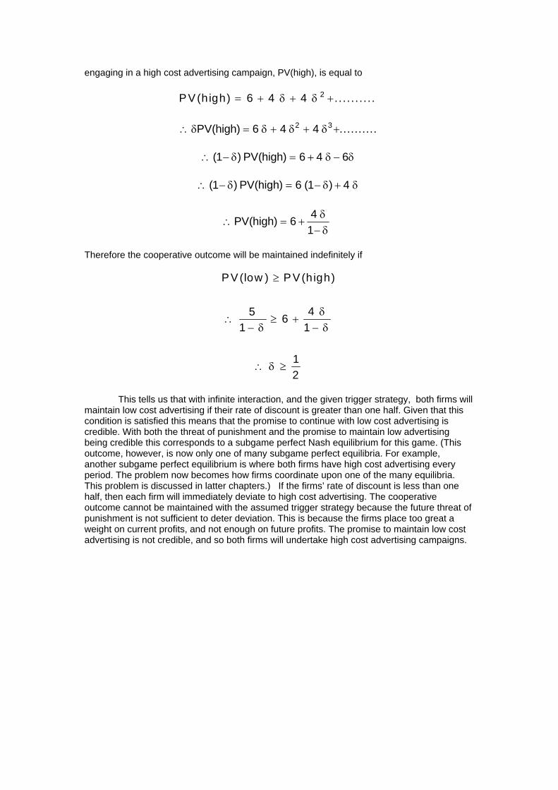
engaging in a high cost advertising campaign, PV(high), is equal to

PV high( ) .. . . . . . . . .= + + +6 4 4 2δ δ

∴ = + + +δ δ δ δPV high( ) ..........6 4 42 3

∴ − = + −( ) ( )1 6 4 6δ δ δPV high

∴ − = − +( ) ( ) ( )1 6 1 4δ δ δPV high

∴ = +−

PV high( ) 6 41δδ

Therefore the cooperative outcome will be maintained indefinitely if

PV low PV high( ) ( )≥

∴−

≥ +−

∴ ≥

51

6 41

12

δδδ

δ

This tells us that with infinite interaction, and the given trigger strategy, both firms will maintain low cost advertising if their rate of discount is greater than one half. Given that this condition is satisfied this means that the promise to continue with low cost advertising is credible. With both the threat of punishment and the promise to maintain low advertising being credible this corresponds to a subgame perfect Nash equilibrium for this game. (This outcome, however, is now only one of many subgame perfect equilibria. For example, another subgame perfect equilibrium is where both firms have high cost advertising every period. The problem now becomes how firms coordinate upon one of the many equilibria. This problem is discussed in latter chapters.) If the firms’ rate of discount is less than one half, then each firm will immediately deviate to high cost advertising. The cooperative outcome cannot be maintained with the assumed trigger strategy because the future threat of punishment is not sufficient to deter deviation. This is because the firms place too great a weight on current profits, and not enough on future profits. The promise to maintain low cost advertising is not credible, and so both firms will undertake high cost advertising campaigns.

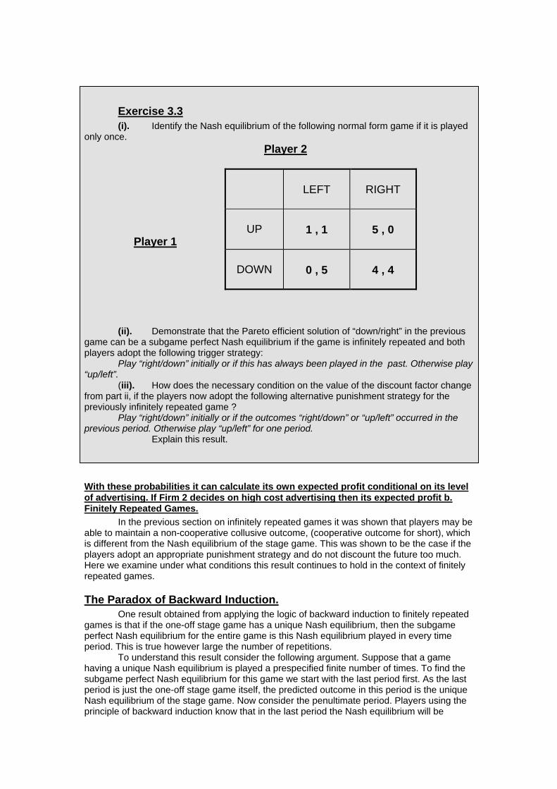
Exercise 3.3 (i). Identify the Nash equilibrium of the following normal form game if it is played only once. Player 1

Player 2

LEFT

RIGHT

UP

1 , 1

5 , 0

DOWN

0 , 5

4 , 4

(ii). Demonstrate that the Pareto efficient solution of “down/right” in the previous game can be a subgame perfect Nash equilibrium if the game is infinitely repeated and both players adopt the following trigger strategy: Play “right/down” initially or if this has always been played in the past. Otherwise play “up/left”. (iii). How does the necessary condition on the value of the discount factor change from part ii, if the players now adopt the following alternative punishment strategy for the previously infinitely repeated game ? Play “right/down” initially or if the outcomes “right/down” or “up/left” occurred in the previous period. Otherwise play “up/left” for one period. Explain this result.

With these probabilities it can calculate its own expected profit conditional on its level of advertising. If Firm 2 decides on high cost advertising then its expected profit b. Finitely Repeated Games. In the previous section on infinitely repeated games it was shown that players may be able to maintain a non-cooperative collusive outcome, (cooperative outcome for short), which is different from the Nash equilibrium of the stage game. This was shown to be the case if the players adopt an appropriate punishment strategy and do not discount the future too much. Here we examine under what conditions this result continues to hold in the context of finitely repeated games.

The Paradox of Backward Induction. One result obtained from applying the logic of backward induction to finitely repeated games is that if the one-off stage game has a unique Nash equilibrium, then the subgame perfect Nash equilibrium for the entire game is this Nash equilibrium played in every time period. This is true however large the number of repetitions. To understand this result consider the following argument. Suppose that a game having a unique Nash equilibrium is played a prespecified finite number of times. To find the subgame perfect Nash equilibrium for this game we start with the last period first. As the last period is just the one-off stage game itself, the predicted outcome in this period is the unique Nash equilibrium of the stage game. Now consider the penultimate period. Players using the principle of backward induction know that in the last period the Nash equilibrium will be

played irrespective of what happens this period. This implies there is no credible threat of future punishment that could induce a player to play other than the unique Nash equilibrium in this penultimate period. All players know this and so again the Nash equilibrium is played. This argument can be applied to all preceding periods until we reach the first period, where again the unique Nash equilibrium is played. The subgame perfect Nash equilibrium for the entire game is simply the Nash equilibrium of the stage game played in every period. This argument implies that a non-cooperative collusive outcome is not possible. This result can be illustrated using the advertising game described above, by assuming that it is only played for two years. In the second year we just have the stage game itself and so the predicted solution is that both firms will incur high advertising costs, and receive an annual profit of £4 million. With the outcome in the second period fully determined the Nash equilibrium for the first period is again that both firms will have high cost advertising campaigns. Similar analysis could have been undertaken for any number of finite repetitions giving the same result that the unique stage game Nash equilibrium will be played in every time period. The subgame perfect solution, therefore, is that both firms will have high cost advertising in both periods. This general result is known as the paradox of backward induction. It is a paradox because of its stark contrast with infinitely repeated games. No matter how many finite number of times we repeat the stage game we never get the same result as if it were infinitely repeated. There is a discontinuity between infinitely repeated games and finitely repeated games, even if the number of repetitions is very large. This is counter intuitive. It is also considered paradoxical because with many repetitions it seams reasonable to assume that players will find some way of coordinating on the Pareto efficient outcome, at least in early periods of the game. The reason for this paradox is that a finite game is qualitatively different from an infinite game. In a finite game the structure of the remaining game changes over time, as we approach the final period. In an infinite game this is not the case. Instead its structure always remains the same wherever we are in the game. In such a game there is no end point from which to begin the logic of backward induction. A number of ways have been suggested in which the paradox of backward induction may be overcome. These include the introduction of bounded rationality, multiple Nash equilibria in the stage game, uncertainty about the future, and uncertainty about other players in the game. These are each examined below.

Bounded Rationality. One suggested way of avoiding the paradox of backward induction is to allow people to be rational but only within certain limits. This is called bounded, or near, rationality. One specific suggestion for how this possibility might be introduced into games is by Radner (1980). Radner allows players to play suboptimal strategies as long as the payoff per period is within epsilon, ε ≥ 0 , of their optimal strategy. This is called an ε - best reply. An ε - equilibrium is correspondingly when all players play ε - best replies. If the number of repetitions is large enough then playing the cooperative outcome, even if it is not a subgame perfect Nash equilibrium, can still be an ε - equilibrium given appropriate trigger strategies. This is demonstrated for the repeated advertising game described above. Assume that both firms adopt the punishment strategy given when considering infinite repetitions, but now the game is only played a finite number of times. If we assume that there is no discounting then the payoff for continuing to play according to this strategy, if the other firm undertakes high cost advertising, is 3 + 4(t-1), where t is the remaining number of periods the firms interact. The payoff for initiating a high cost advertising campaign is at most 6 + 4(t-1). Deviating from the punishment strategy therefore yields a net benefit of 3. This is equal to 3/t per period. If players are boundedly rational as defined by Radner then the cooperative outcome is an ε - equilibrium if ε > 3/t. This will be satisfied for any value of ε , provided the remaining number of periods is great enough. Given a large number of repetitions cooperation, which in this example means low cost advertising, will be observed in the initial periods of the game. Although interesting to analyse the effects of bounded rationality in repeated games, it is not clear that Radner’s suggestion is the best way of doing this. For example, Friedman (1986) argues that bounded rationality might imply that people only calculate optimal strategies for a limited number of periods. If this is true then the game becomes shorter, and the result of backward induction more likely. Furthermore if people do not fully rationalise we should consider why. If it is due to calculation costs, then these costs should be added to the

structure of the game itself. This is an area of on going research.

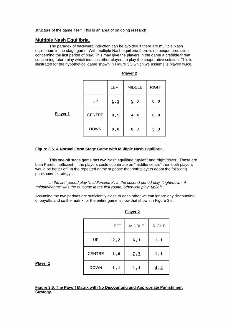
Multiple Nash Equilibria. The paradox of backward induction can be avoided if there are multiple Nash equilibrium in the stage game. With multiple Nash equilibria there is no unique prediction concerning the last period of play. This may give the players in the game a credible threat concerning future play which induces other players to play the cooperative solution. This is illustrated for the hypothetical game shown in Figure 3.5 which we assume is played twice. Player 1

Player 2

LEFT

MIDDLE

RIGHT

UP

1 , 1

5 , 0

0 , 0

CENTRE

0 , 5

4 , 4

0 , 0

DOWN

0 , 0

0 , 0

3 , 3

Figure 3.5. A Normal Form Stage Game with Multiple Nash Equilibria. This one-off stage game has two Nash equilibria “up/left” and “right/down”. These are both Pareto inefficient. If the players could coordinate on “middle/ centre” then both players would be better off. In the repeated game suppose that both players adopt the following punishment strategy : In the first period play “middle/centre”. In the second period play “right/down” if “middle/centre” was the outcome in the first round, otherwise play “up/left”. Assuming the two periods are sufficiently close to each other we can ignore any discounting of payoffs and so the matrix for the entire game is now that shown in Figure 3.6.

Player 1

Player 2

LEFT

MIDDLE

RIGHT

UP

2 , 2

6 , 1

1 , 1

CENTRE

1 , 6

7 , 7

1 , 1

DOWN

1 , 1

1 , 1

4 , 4

Figure 3.6. The Payoff Matrix with No Discounting and Appropriate Punishment Strategy.

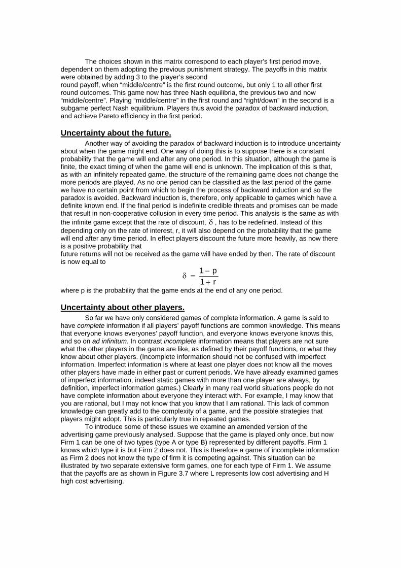
The choices shown in this matrix correspond to each player’s first period move, dependent on them adopting the previous punishment strategy. The payoffs in this matrix were obtained by adding 3 to the player’s second round payoff, when “middle/centre” is the first round outcome, but only 1 to all other first round outcomes. This game now has three Nash equilibria, the previous two and now “middle/centre”. Playing “middle/centre” in the first round and “right/down” in the second is a subgame perfect Nash equilibrium. Players thus avoid the paradox of backward induction, and achieve Pareto efficiency in the first period.

Uncertainty about the future. Another way of avoiding the paradox of backward induction is to introduce uncertainty about when the game might end. One way of doing this is to suppose there is a constant probability that the game will end after any one period. In this situation, although the game is finite, the exact timing of when the game will end is unknown. The implication of this is that, as with an infinitely repeated game, the structure of the remaining game does not change the more periods are played. As no one period can be classified as the last period of the game we have no certain point from which to begin the process of backward induction and so the paradox is avoided. Backward induction is, therefore, only applicable to games which have a definite known end. If the final period is indefinite credible threats and promises can be made that result in non-cooperative collusion in every time period. This analysis is the same as with the infinite game except that the rate of discount, δ , has to be redefined. Instead of this depending only on the rate of interest, r, it will also depend on the probability that the game will end after any time period. In effect players discount the future more heavily, as now there is a positive probability that future returns will not be received as the game will have ended by then. The rate of discount is now equal to

δ =−+

11

pr

where p is the probability that the game ends at the end of any one period.

Uncertainty about other players. So far we have only considered games of complete information. A game is said to have complete information if all players’ payoff functions are common knowledge. This means that everyone knows everyones’ payoff function, and everyone knows everyone knows this, and so on ad infinitum. In contrast incomplete information means that players are not sure what the other players in the game are like, as defined by their payoff functions, or what they know about other players. (Incomplete information should not be confused with imperfect information. Imperfect information is where at least one player does not know all the moves other players have made in either past or current periods. We have already examined games of imperfect information, indeed static games with more than one player are always, by definition, imperfect information games.) Clearly in many real world situations people do not have complete information about everyone they interact with. For example, I may know that you are rational, but I may not know that you know that I am rational. This lack of common knowledge can greatly add to the complexity of a game, and the possible strategies that players might adopt. This is particularly true in repeated games. To introduce some of these issues we examine an amended version of the advertising game previously analysed. Suppose that the game is played only once, but now Firm 1 can be one of two types (type A or type B) represented by different payoffs. Firm 1 knows which type it is but Firm 2 does not. This is therefore a game of incomplete information as Firm 2 does not know the type of firm it is competing against. This situation can be illustrated by two separate extensive form games, one for each type of Firm 1. We assume that the payoffs are as shown in Figure 3.7 where L represents low cost advertising and H high cost advertising.

Firm 1 is Type A Firm 1 is Type B

1A

H

L

2

2

H

H

L

L

1B

H

L

H

H

L

L

(4 , 4)

(6 , 3)(3 , 4)

(5 , 5)

(0 , 4)

(2 , 3)(3 , 4)

(5 , 5)

2

2

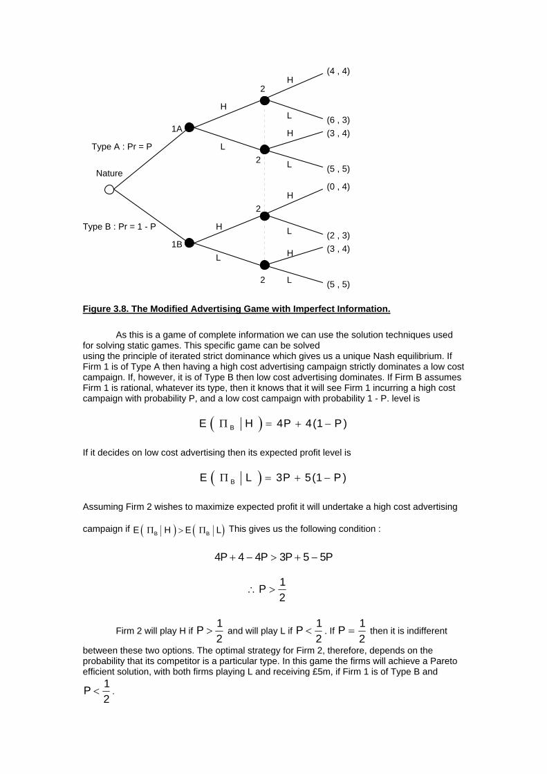
Figure 3.7. The Modified Advertising Game with Incomplete Information. There are two changes to the firms’ payoffs as compared to the previous advertising game represented in Figure 3.4. 1. Firm 1 has the same payoffs as before if it is type A, but type B receives £4m less per year if it undertakes a high cost advertising campaign. This can reflect either a genuine cost differential between the two types of firm, or a difference in preferences, i.e. type B might have moral objections against high powered advertising. 2. Firm 2 now receives £2m per year less than before if it undertakes a high cost advertising campaign, and firm 1 has a low cost campaign. This might, for example, be due to a production constraint that precludes the firm benefiting from higher demand for its goods. Its other payoffs remain the same. The effect of this change, and the reason it was made, is that Firm 2 no longer has the strictly dominant strategy of high cost advertising. This implies that its behaviour can depend on which type of competitor it thinks it is playing against. This is the result we wish to show. One immediate problem of solving games with incomplete information is that the techniques so far discussed cannot be directly applied to these situations. This is because they all make the fundamental assumption that players know which game they are playing. This is not the case if players are unsure what their opponents are like. As Figure 3.7 illustrates Firm 2 does not know which of the two extensive form games it is playing. Fortunately Harsanyi (1967,1968) showed that games with incomplete information, can be transformed into games of complete but imperfect information. As we have already examined such games the previous solution techniques can be applied to these transformed games. The transformation is done by assuming that Nature determines each player’s type, and hence payoff function, according to a probability distribution. This probability distribution is assumed to be common knowledge. Each player is assumed to know their own type but not always the type of other players in the game. This is now a game of complete but imperfect information as not all players observe Nature’s initial moves. If we assume that Nature assigns Type A to Firm 1 with probability P and Type B with probability 1 - P then this situation can now be represented by just the one extensive form game. This is shown in Figure 3.8.

1A

H

L

2

2

H

H

L

L

1B

H

L

H

H

L

L

(4 , 4)

(6 , 3)(3 , 4)

(5 , 5)

(0 , 4)

(2 , 3)(3 , 4)

(5 , 5)

Nature

2

2

Type A : Pr = P

Type B : Pr = 1 - P

Figure 3.8. The Modified Advertising Game with Imperfect Information. As this is a game of complete information we can use the solution techniques used for solving static games. This specific game can be solved using the principle of iterated strict dominance which gives us a unique Nash equilibrium. If Firm 1 is of Type A then having a high cost advertising campaign strictly dominates a low cost campaign. If, however, it is of Type B then low cost advertising dominates. If Firm B assumes Firm 1 is rational, whatever its type, then it knows that it will see Firm 1 incurring a high cost campaign with probability P, and a low cost campaign with probability 1 - P. level is

( )E H P PBΠ = + −4 4 1( )

If it decides on low cost advertising then its expected profit level is

( )E L P PBΠ = + −3 5 1( )

Assuming Firm 2 wishes to maximize expected profit it will undertake a high cost advertising

campaign if ( ) ( )E H E LB BΠ Π> This gives us the following condition :

4 4 4 3 5 5P P P P+ − > + −

∴ >P 12

Firm 2 will play H if P >12

and will play L if P <12

. If P =12

then it is indifferent

between these two options. The optimal strategy for Firm 2, therefore, depends on the probability that its competitor is a particular type. In this game the firms will achieve a Pareto efficient solution, with both firms playing L and receiving £5m, if Firm 1 is of Type B and

P <12

.

The above illustration has shown that incomplete information can lead to player’s achieving a Pareto efficient outcome. However, in this one-off game, this only happened if Firm 1 was of a type that always undertakes a low cost advertising campaign. If the game is repeated a finite number of times this restriction need not always apply for the outcome to be Pareto efficient. Unfortunately solving such repeated games is far from straight forward. This is because of two added complications. The first complication is that in dynamic games of incomplete information, players may be able to learn what other players are like by observing their past actions. This gives players the opportunity to try and influence other players’ expectations of their type by modifying their actions. For example, consider what might happen if the above incomplete information advertising game is repeated a finite number of times. If Firm 1 can convince Firm 2 that it is Type B, then Firm 2 will incur low advertising costs and so increase Firm 1’s profits. The only way that Firm 1 can convince the other firm that it is Type B is to play as a Type B firm would play. This is true even if firm 1 is actually Type A. Thus it is possible that players might seek to conceal their true identity, so as to gain a reputation for being something they are not. Gaining such a reputation can be thought of as an investment. Although obtaining a reputation for something you are not will be costly in the short - run, it brings with it the expectation of higher future returns. The second complication, is that players know that other players might have this incentive to conceal their true identity. This will influence how they update their probability assessment of the other player’s type conditional on observing their actions. The other player will in turn take this into account when determining their behaviour, and so on. Only recently have such games been explicitly solved by game theorists and applied to economic situations. The equilibrium concept often used in such games is Bayesian Subgame Perfect Nash Equilibrium, or Bayesian Perfect for short. This type of equilibrium satisfies two conditions : (i) It is subgame perfect, in that no incredible threats or promises are made or believed. (ii) The players update their beliefs rationally in accordance with Bayes’ Theorem. (An alternative equilibrium concept used is sequential equilibrium. This was developed by Kreps and Wilson (1982b) and is a slightly stronger condition than Bayesian Perfect equilibrium with regard to the consistency of the solution. In many cases, however, the two concepts yield the same solution.) Bayes’ Theorem is explained in Appendix 3.1. The relevance of Bayesian Perfect equilibrium is that even very small amounts of uncertainty concerning the type of player you are playing against can be greatly magnified in repeated games. This alters the incentives faced by players in the game, and often leads to the prediction that the Pareto optimal solution is played in early stages of the game. In this way the paradox of backward induction is overcome. To illustrate this possibility we discuss the centipede game developed by Rosenthal (1981). Consider the extensive form game shown in Figure 3.9.

1 2

D

A

D

A

(1,1) (0,3)

1 2

D

A

D

A 1 2

D

A

D

A (100,100).........

(98,101)(99,99)(97,100)(98,98)

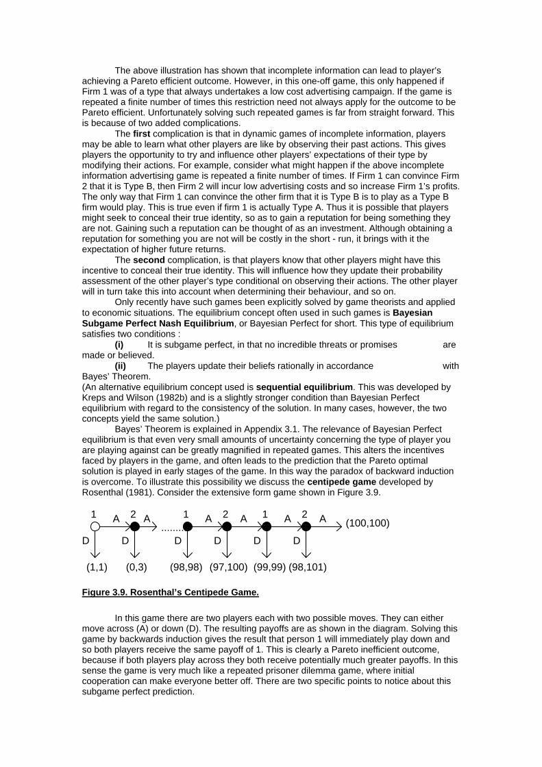
Figure 3.9. Rosenthal’s Centipede Game. In this game there are two players each with two possible moves. They can either move across (A) or down (D). The resulting payoffs are as shown in the diagram. Solving this game by backwards induction gives the result that person 1 will immediately play down and so both players receive the same payoff of 1. This is clearly a Pareto inefficient outcome, because if both players play across they both receive potentially much greater payoffs. In this sense the game is very much like a repeated prisoner dilemma game, where initial cooperation can make everyone better off. There are two specific points to notice about this subgame perfect prediction.

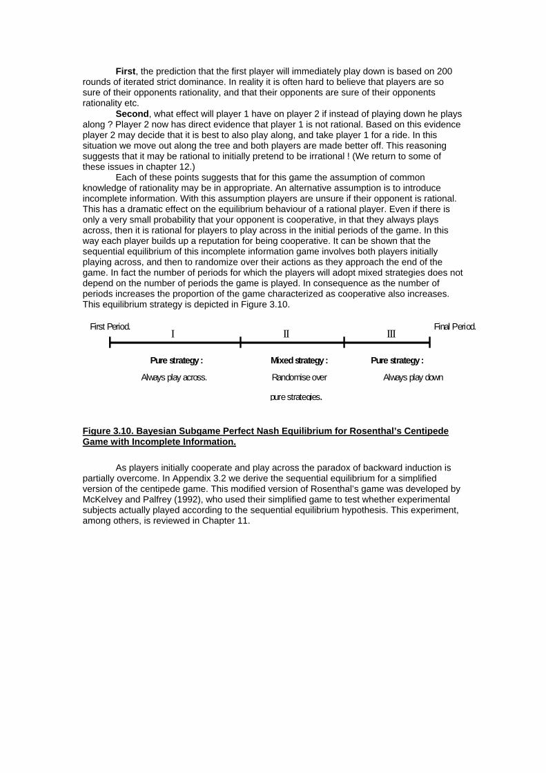
First, the prediction that the first player will immediately play down is based on 200 rounds of iterated strict dominance. In reality it is often hard to believe that players are so sure of their opponents rationality, and that their opponents are sure of their opponents rationality etc. Second, what effect will player 1 have on player 2 if instead of playing down he plays along ? Player 2 now has direct evidence that player 1 is not rational. Based on this evidence player 2 may decide that it is best to also play along, and take player 1 for a ride. In this situation we move out along the tree and both players are made better off. This reasoning suggests that it may be rational to initially pretend to be irrational ! (We return to some of these issues in chapter 12.) Each of these points suggests that for this game the assumption of common knowledge of rationality may be in appropriate. An alternative assumption is to introduce incomplete information. With this assumption players are unsure if their opponent is rational. This has a dramatic effect on the equilibrium behaviour of a rational player. Even if there is only a very small probability that your opponent is cooperative, in that they always plays across, then it is rational for players to play across in the initial periods of the game. In this way each player builds up a reputation for being cooperative. It can be shown that the sequential equilibrium of this incomplete information game involves both players initially playing across, and then to randomize over their actions as they approach the end of the game. In fact the number of periods for which the players will adopt mixed strategies does not depend on the number of periods the game is played. In consequence as the number of periods increases the proportion of the game characterized as cooperative also increases. This equilibrium strategy is depicted in Figure 3.10.

Pure strategy : Mixed strategy : Pure strategy :

Always play down Always play across.

First Period. Final Period.

Randomise over

purestrategies.

I II III

Figure 3.10. Bayesian Subgame Perfect Nash Equilibrium for Rosenthal’s Centipede Game with Incomplete Information. As players initially cooperate and play across the paradox of backward induction is partially overcome. In Appendix 3.2 we derive the sequential equilibrium for a simplified version of the centipede game. This modified version of Rosenthal’s game was developed by McKelvey and Palfrey (1992), who used their simplified game to test whether experimental subjects actually played according to the sequential equilibrium hypothesis. This experiment, among others, is reviewed in Chapter 11.

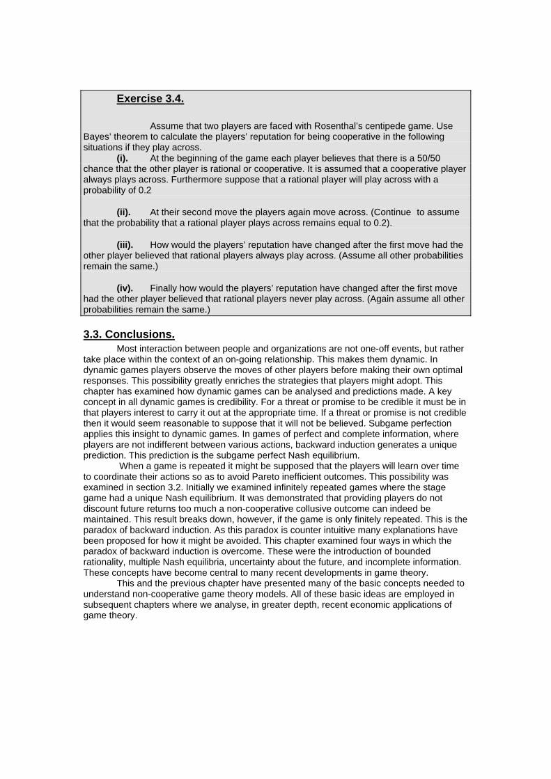
Exercise 3.4.

Assume that two players are faced with Rosenthal’s centipede game. Use Bayes’ theorem to calculate the players’ reputation for being cooperative in the following situations if they play across. (i). At the beginning of the game each player believes that there is a 50/50 chance that the other player is rational or cooperative. It is assumed that a cooperative player always plays across. Furthermore suppose that a rational player will play across with a probability of 0.2

(ii). At their second move the players again move across. (Continue to assume that the probability that a rational player plays across remains equal to 0.2).

(iii). How would the players’ reputation have changed after the first move had the other player believed that rational players always play across. (Assume all other probabilities remain the same.)

(iv). Finally how would the players’ reputation have changed after the first move had the other player believed that rational players never play across. (Again assume all other probabilities remain the same.)

3.3. Conclusions. Most interaction between people and organizations are not one-off events, but rather take place within the context of an on-going relationship. This makes them dynamic. In dynamic games players observe the moves of other players before making their own optimal responses. This possibility greatly enriches the strategies that players might adopt. This chapter has examined how dynamic games can be analysed and predictions made. A key concept in all dynamic games is credibility. For a threat or promise to be credible it must be in that players interest to carry it out at the appropriate time. If a threat or promise is not credible then it would seem reasonable to suppose that it will not be believed. Subgame perfection applies this insight to dynamic games. In games of perfect and complete information, where players are not indifferent between various actions, backward induction generates a unique prediction. This prediction is the subgame perfect Nash equilibrium. When a game is repeated it might be supposed that the players will learn over time to coordinate their actions so as to avoid Pareto inefficient outcomes. This possibility was examined in section 3.2. Initially we examined infinitely repeated games where the stage game had a unique Nash equilibrium. It was demonstrated that providing players do not discount future returns too much a non-cooperative collusive outcome can indeed be maintained. This result breaks down, however, if the game is only finitely repeated. This is the paradox of backward induction. As this paradox is counter intuitive many explanations have been proposed for how it might be avoided. This chapter examined four ways in which the paradox of backward induction is overcome. These were the introduction of bounded rationality, multiple Nash equilibria, uncertainty about the future, and incomplete information. These concepts have become central to many recent developments in game theory. This and the previous chapter have presented many of the basic concepts needed to understand non-cooperative game theory models. All of these basic ideas are employed in subsequent chapters where we analyse, in greater depth, recent economic applications of game theory.

3.4. Solutions to Exercises.

Exercise 3.1. Using the principle of backward induction we start at the end of the game and work backwards ruling out strategies that rational players would not play. If the game reaches player three’s decision node then he receives with certainty a payoff of 7 if he plays “up” or 9 if he plays “down”. Assuming this player is rational he will play “down”, and so we can exclude his strategy of “up”. Moving back along this branch we reach player 2’s node after player 1 has moved “down”. If we assume player 2 believes player 3 is rational then he anticipates receiving a payoff of 8 if he moves “up”, and 1 if he moves “down”. If player 2 is also assumed to be rational then at this decision node he will play “up” and we can exclude “down” from this node. Player 2 also has a decision node following player 1 moving “up”. By considering player 2’s certain payoff’s following this decision we can exclude “up” and “down” as we have already assumed this player is rational. We now only have to solve player 1’s move at the start of the game. There are now only two remaining payoffs for the game as a whole. If we assume player 1 believes player 2 is rational then he will anticipate a payoff of 3 if he moves “up”. Further if we assume that player 1 believes that player 2 believes that player 3 is rational then he will anticipate a payoff of 6 if he moves “down”. With these assumptions we can exclude player 1 moving “up”. With the above assumptions we are left with one remaining payoff vector corresponding to the subgame perfect Nash equilibrium. This equilibrium is that player 1 moves “down” followed by player 2 moving “up”, and finally player 3 choosing to play “down”. We derive the same solution if we assume all players in the game are rational and that this is common knowledge. This assumption is stronger than absolutely necessary, but for convenience it is typically made when applying the principle of backward induction.

Exercise 3.2. For the extensive form game given in this exercise there are two Nash equilibria, but only one is perfect. To identify these Nash equilibria we first convert the game into a normal form game. Player A has only two strategies A1 or A2. However player 2 has four available strategies because he can condition his actions on what he observes player A does. Player 2’s strategies are, therefore, to always play B1, to always play B2, do the same as player A, or do the opposite. This gives us the normal form game shown in Figure 3.11. Player A

Player B

ALWAYS B1

ALWAYS B2

SAME AS

A

OPPOSITE

TO A

A1

6 , 8

8 , 4

6 , 8

8 , 4

A2

4 , 6

7 , 7

7 , 7

4 , 6

Figure 3.11. Using the two stage procedure for finding pure strategy Nash equilibria we can identify that “A1/ALWAYS B1” and “A2/SAME AS A” are both Nash equilibria. The concept of

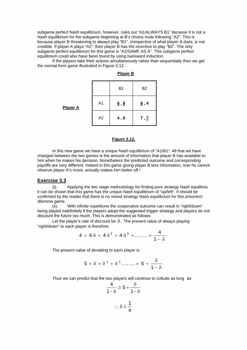
subgame perfect Nash equilibrium, however, rules out “A1/ALWAYS B1” because it is not a Nash equilibrium for the subgame beginning at B’s choice node following “A2”. This is because player B threatening to always play “B1”, irrespective of what player A does, is not credible. If player A plays “A2”, then player B has the incentive to play “B2”. The only subgame perfect equilibrium for this game is “A2/SAME AS A”. This subgame perfect equilibrium could also have been found by using backward induction. If the players take their actions simultaneously rather than sequentially then we get the normal form game illustrated in Figure 3.12. Player A

Player B

B1

B2

A1

6 , 8

8 , 4

A2

4 , 6

7 , 7

Figure 3.12. In this new game we have a unique Nash equilibrium of “A1/B1”. All that we have changed between the two games is the amount of information that player B has available to him when he makes his decision. Nonetheless the predicted outcome and corresponding payoffs are very different. Indeed in this game giving player B less information, now he cannot observe player A’s move, actually makes him better off !

Exercise 3.3 (i). Applying the two stage methodology for finding pure strategy Nash equilibria it can be shown that this game has the unique Nash equilibrium of “up/left”. It should be confirmed by the reader that there is no mixed strategy Nash equilibrium for this prisoners’ dilemma game. (ii). With infinite repetitions the cooperative outcome can result in “right/down” being played indefinitely if the players adopt the suggested trigger strategy and players do not discount the future too much. This is demonstrated as follows. Let the player’s rate of discount be δ . The present value of always playing “right/down” to each player is therefore

4 4 4 4 41

2 3+ + + + =−

δ δ δδ

. . . . . . .

The present value of deviating to each player is

5 51

2 3+ + + = +−

δ δ δδδ

........

Thus we can predict that the two players will continue to collude as long as 4

15

1−≥ +

−δδδ

∴ ≥δ14

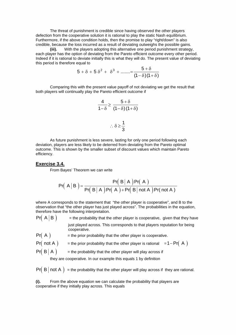
The threat of punishment is credible since having observed the other players defection from the cooperative solution it is rational to play the static Nash equilibrium. Furthermore, if the above condition holds, then the promise to play “right/down” is also credible, because the loss incurred as a result of deviating outweighs the possible gains. (iii). With the players adopting this alternative one period punishment strategy, each player has the option of deviating from the Pareto efficient outcome every other period. Indeed if it is rational to deviate initially this is what they will do. The present value of deviating this period is therefore equal to

5 5 51 1

2 3+ + + + =+

− +δ δ δ

δδ δ

.......( )( )

Comparing this with the present value payoff of not deviating we get the result that both players will continually play the Pareto efficient outcome if

41

51 1

13

−≥

+− +

∴ ≥

δδ

δ δ

δ

( ) ( )

As future punishment is less severe, lasting for only one period following each deviation, players are less likely to be deterred from deviating from the Pareto optimal outcome. This is shown by the smaller subset of discount values which maintain Pareto efficiency.

Exercise 3.4. From Bayes’ Theorem we can write

( ) ( ) ( )( ) ( ) ( )Pr

Pr PrPr Pr Pr Pr( )

A BB A A

B A A B not A not A=

+

where A corresponds to the statement that “the other player is cooperative”, and B to the observation that “the other player has just played across”. The probabilities in the equation, therefore have the following interpretation.

( )Pr A B = the probability that the other player is cooperative, given that they have

just played across. This corresponds to that players reputation for being cooperative.

( )Pr A = the prior probability that the other player is cooperative.

( )Pr not A = the prior probability that the other player is rational = ( )1−Pr A

( )Pr B A = the probability that the other player will play across if

they are cooperative. In our example this equals 1 by definition

( )Pr B not A = the probability that the other player will play across if they are rational.

(i). From the above equation we can calculate the probability that players are cooperative if they initially play across. This equals

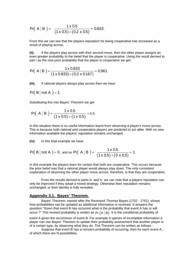
( )Pr A B = ( ) ( )

1 0 51 0 5 0 2 0 5

0 833xx x

.. . .

.+

= .

From this we can see that the players reputation for being cooperative has increased as a result of playing across.

(ii). If the players play across with their second move, then the other player assigns an even greater probability to the belief that the player is cooperative. Using the result derived to part i as the new prior probability that the player is cooperative we get :

( ) ( ) ( )Pr .. . .

.A B xx x

=+

=1 0 833

1 0 833 0 2 01670 961

(iii). If rational players always play across then we have

( )Pr B not A = 1.

Substituting this into Bayes’ Theorem we get

( ) ( ) ( )Pr .

. .A B x

x x=

+1 0 5

1 0 5 1 0 5 = 0.5.

In this situation there is no useful information learnt from observing a player’s move across. This is because both rational and cooperative players are predicted to act alike. With no new information available the players’ reputation remains unchanged.

(iv). In this final example we have

( )Pr B not A = 0 , and so ( )Pr A B = ( ) ( )1 0 5

1 0 5 0 0 51x

x x.

. .+= .

In this example the players learn for certain that both are cooperative. This occurs because the prior belief was that a rational player would always play down. The only consistent explanation of observing the other player move across, therefore, is that they are cooperative.

From the results derived to parts iii. and iv. we can note that a players reputation can only be improved if they adopt a mixed strategy. Otherwise their reputation remains unchanged, or their identity is fully revealed.

Appendix 3.1. Bayes’ Theorem. Bayes’ Theorem, named after the Reverend Thomas Bayes (1702 - 1761), shows how probabilities can be updated as additional information is received. It answers the question “Given that event B has occurred what is the probability that event A has or will occur ?” This revised probability is written as ( )Pr A B . It is the conditional probability of

event A given the occurrence of event B. For example in games of incomplete information a player can use Bayes’ Theorem to update their probability assessment that another player is of a certain type, by observing what they do. The Theorem can be written as follows : Suppose that event B has a nonzero probability of occurring, then for each event Ai , of which there are N possibilities,

Pr ( )P r( ) . P r ( )

P r ( ) . P r ( )A B

B A A

B A Ai

i

ii

N=

=∑

1

For example, if there are only two possible types of a certain player, A1 and A2, the updated probability for each type, given that this player has undertaken an action B is :

P r ( )P r ( ) . P r ( )

P r ( ) . P r ( ) P r ( ) . P r ( )A B

B A AB A A B A A1

1

1 1 2 2

=+

and

P r ( )P r ( ) . P r ( )

P r ( ) . P r ( ) P r ( ) . P r ( )A B

B A AB A A B A A2

2

1 1 2 2

=+

The probabilities used on the right hand side of these expressions are called “prior probabilities”, and are determined before event B occurs. The updated probabilities Pr ( )A Bi are called “posterior probabilities”. In repeated games these posterior probabilities would then be used as the prior probabilities of Pr ( )Ai in subsequent periods. Proof of Bayes’ Theorem. From the nature of conditional probabilities it is true that ( )Pr Pr ( ) . Pr ( )A and B B A Ai i i= (1.) and ( )Pr Pr ( ) . Pr ( )A and B A B Bi i= (2.) From (2.) we get

Pr ( ) Pr ( )Pr ( )

A B A and BBi

i= (3.)

Substituting in for Pr ( )A and Bi from equation (1.) gives

Pr ( )Pr ( ) . Pr ( )

Pr ( )A B

B A ABi

i i= (4.)

Multiplying through by Pr ( )B yields Pr ( ) . Pr ( ) Pr ( ) . Pr ( )B A B B A Ai i i= (5.)

Summing both sides over the index i gives

Pr ( ) . Pr ( ) Pr ( ) . Pr ( )B A B B A Aii

N

i ii

N

= =∑ ∑=

1 1 (6.)

Since the events { }A AN1,....., are mutually exclusive and exhaustive we know that

Pr ( )A Bii

N

=∑ =

11 (7.)

Substituting (7.) into (6.) we have

Pr ( ) Pr ( ) . Pr ( )B B A Ai ii

N

==∑

1 (8.)

Substituting (8.) into (4.) gives us Bayes’ Theorem. This completes the proof.

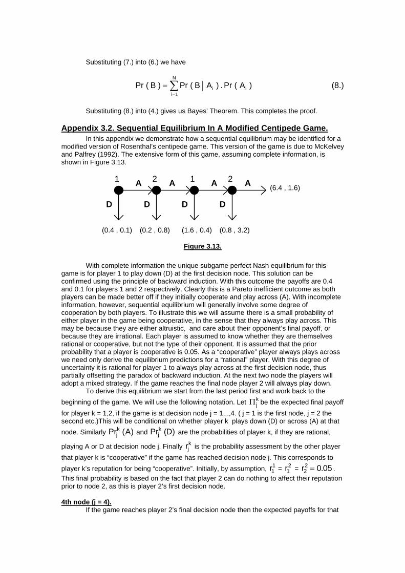
Appendix 3.2. Sequential Equilibrium In A Modified Centipede Game. In this appendix we demonstrate how a sequential equilibrium may be identified for a modified version of Rosenthal’s centipede game. This version of the game is due to McKelvey and Palfrey (1992). The extensive form of this game, assuming complete information, is shown in Figure 3.13.

1 2

D

A

D

A 1 2

D

A

D

A

(0.8 , 3.2)(1.6 , 0.4)(0.2 , 0.8)(0.4 , 0.1)

(6.4 , 1.6)

Figure 3.13. With complete information the unique subgame perfect Nash equilibrium for this game is for player 1 to play down (D) at the first decision node. This solution can be confirmed using the principle of backward induction. With this outcome the payoffs are 0.4 and 0.1 for players 1 and 2 respectively. Clearly this is a Pareto inefficient outcome as both players can be made better off if they initially cooperate and play across (A). With incomplete information, however, sequential equilibrium will generally involve some degree of cooperation by both players. To illustrate this we will assume there is a small probability of either player in the game being cooperative, in the sense that they always play across. This may be because they are either altruistic, and care about their opponent’s final payoff, or because they are irrational. Each player is assumed to know whether they are themselves rational or cooperative, but not the type of their opponent. It is assumed that the prior probability that a player is cooperative is 0.05. As a “cooperative” player always plays across we need only derive the equilibrium predictions for a “rational” player. With this degree of uncertainty it is rational for player 1 to always play across at the first decision node, thus partially offsetting the paradox of backward induction. At the next two node the players will adopt a mixed strategy. If the game reaches the final node player 2 will always play down. To derive this equilibrium we start from the last period first and work back to the beginning of the game. We will use the following notation. Let Π j

k be the expected final payoff for player k = 1,2, if the game is at decision node j = 1,..,4. ( j = 1 is the first node, j = 2 the second etc.)This will be conditional on whether player k plays down (D) or across (A) at that node. Similarly Pr ( )j

k A and Pr ( )jk D are the probabilities of player k, if they are rational,

playing A or D at decision node j. Finally rjk is the probability assessment by the other player

that player k is “cooperative” if the game has reached decision node j. This corresponds to player k’s reputation for being “cooperative”. Initially, by assumption, r1

1 = r12 = r2

2 0 05= . . This final probability is based on the fact that player 2 can do nothing to affect their reputation prior to node 2, as this is player 2’s first decision node. 4th node (j = 4). If the game reaches player 2’s final decision node then the expected payoffs for that

player are Π42 3 2( ) .D = and Π4

2 16( ) .A = . As down strictly dominates across it is clear that if player 2 is rational they will always play down. This pure strategy prediction implies that Pr ( )4

2 0A = and Pr ( )42 1D = for a rational player.

3rd node (j = 3). Based on the results derived for node 4 the expected payoffs for player 1 if the game reaches node 3 are Π3

1 16( ) .D = and Π31

32

320 8 1 6 4( ) . ( ) .A r r= − + . If one of these

expected payoffs is greater than the other then player 1 will play a pure strategy at this node. If, however, these expected values are equal then player 1(if rational) is indifferent between playing across or down. In this situation player 1 can play a mixed strategy at this node. This

will occur when r32 1

7= . Player 1 will only play a mixed strategy at this node if player 2 has

previously enhanced their reputation for being “cooperative”. This, in turn, can only happen if player 2 has played a mixed strategy at decision node 2. Specifically using Bayes’ Theorem we can calculate the implied probability of player 2 playing down at node 2 in order to induce player 1 to play a mixed strategy at node 3. Thus

[ ]

[ ]

r rr D r

D

32 2

2

22

22

22

22

1 117

0 050 05 1 0 95

17

=+ − −

=

∴+ −

=

Pr ( ) ( )

.. Pr ( ) .

∴ =Pr ( ) . .2

2 0 684D

∴ =Pr ( ) .22 0 316A

Player 1 will, therefore, adopt a mixed strategy at node 3 if player 2 has plays this mixed strategy at node 2. 2nd node (j = 2). At node 2 we can derive the following expected payoffs for player 2. Π2

2 0 8( ) .D = and

[ ]Π22

12

12

31

31

31

31

21

31

3 2 1 0 4 1

3 2 2 8 2 8

( ) . ( )Pr ( ) . ( )Pr ( )

. . Pr ( ) . Pr ( )

A r r A r D

D r D

= + − + −

= − +

Again if either of these expected payoffs is greater than the other then player 2 will adopt a pure strategy. If these expected payoffs are equal then a player 2 (if rational) can adopt a

mixed strategy at this node. This will occur when Pr ( )( )3

1

21

67 1

Dr

=−

. Given that r21 is

sufficiently small, player 2 will use a mixed strategy at node 2 if player 1 is anticipated to play the appropriate mixed strategy at node 3. This is similar to the prediction derived for node 3. The mixed strategies at nodes 2 and 3 are self supporting in equilibrium.

If we assume that player 1 always plays across at node 1(this assumption is validated below) then from Bayes’ Theorem r2

1 0 05= . . From the previous equation, therefore, player 2

will play a mixed strategy at node 2 if Pr ( ) .31 0 902D = and Pr ( ) .3

1 0 098A = . 1st node (j = 1). In order to justify the use of mixed strategies derived above for nodes 2 and 3 all that is needed now is to demonstrate that, given these predictions, player 1 will play across at this first decision node. Again the expected payoffs for player 1 at this node are given as Π1

1 0 4( ) .D = and

[ ]

[ ]

[ ]

Π11

12

22

12

12

22

31

12

12

22

31

12

12

12

22

31

0 2 1 16 1

0 8 1 1

6 4 1

( ) . ( )Pr ( ) . ( )Pr ( ) Pr ( )

. ( )Pr ( ) Pr ( ) ( )

. ( )Pr ( ) Pr ( )

A r D r r A D

r r A A r

r r A A

= − + + −

+ + − −

+ + −

Given the previous mixed strategy predictions we can calculate that Π11 1036( ) . .A = For

player 1 playing across dominates playing down at this node, and so player 1 will always play across irrespective of their type. This pure strategy prediction implies that Pr ( )1

1 1A = and

Pr ( )11 0D = for a rational player.

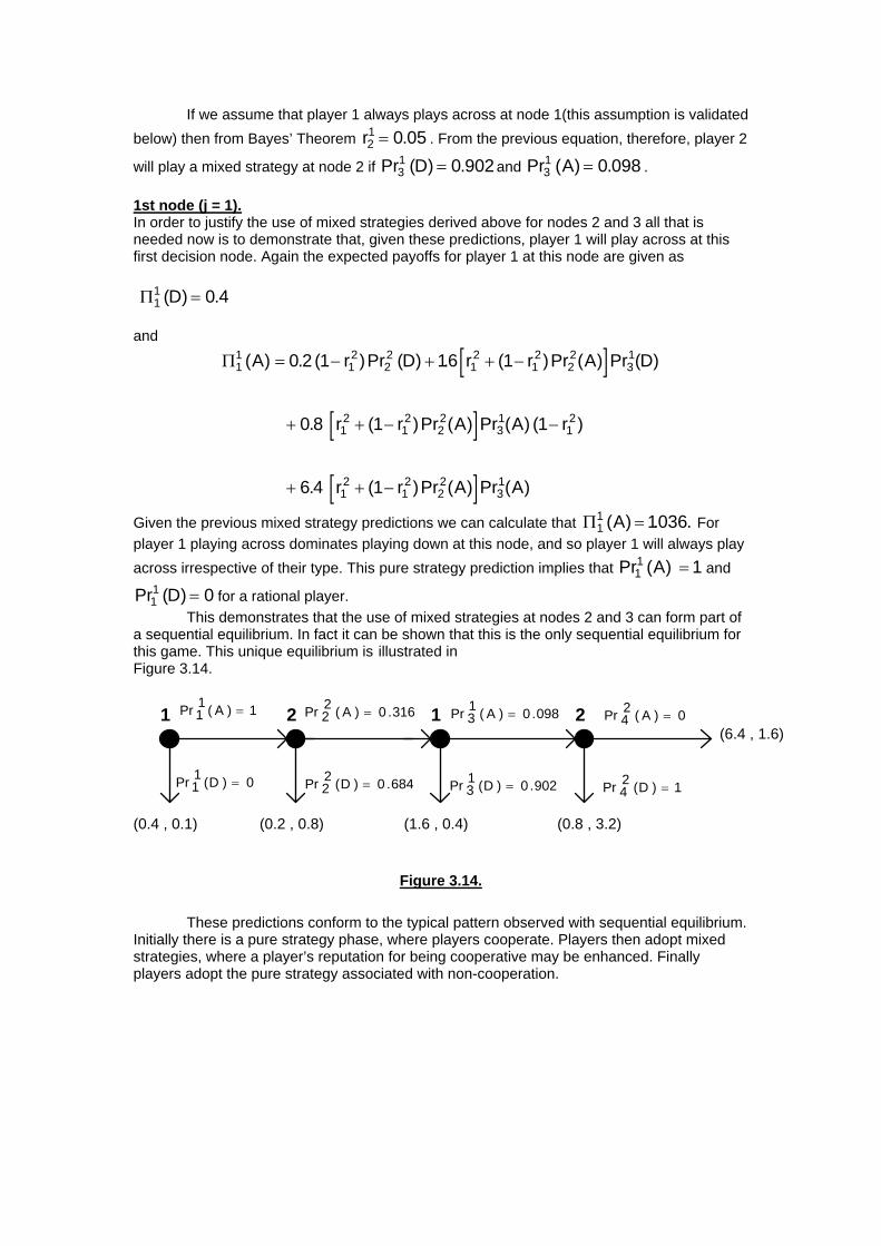
This demonstrates that the use of mixed strategies at nodes 2 and 3 can form part of a sequential equilibrium. In fact it can be shown that this is the only sequential equilibrium for this game. This unique equilibrium is illustrated in Figure 3.14.

1 2 1 2

(0.8 , 3.2)(1.6 , 0.4)(0.2 , 0.8)(0.4 , 0.1)

(6.4 , 1.6)Pr ( )1

1 1A =

Pr ( )11 0D =

Pr ( ) .22 0 316A =

Pr ( ) .22 0 684D =

Pr ( ) .31 0 098A =

Pr ( ) .31 0 902D =

Pr ( )42 0A =

Pr ( )42 1D =

Figure 3.14. These predictions conform to the typical pattern observed with sequential equilibrium. Initially there is a pure strategy phase, where players cooperate. Players then adopt mixed strategies, where a player’s reputation for being cooperative may be enhanced. Finally players adopt the pure strategy associated with non-cooperation.

Further Reading. Aumann, R. and S. Hart (1992) Handbook of Game Theory with Economic Applications, New York : North-Holland. Bierman, H. S. and L. Fernandez (1993) Game Theory with Economic Applications, Reading, Mass. : Addison Wesley. Dixit, A. and B. J. Nalebuff (1991) Thinking Strategically : The Competitive Edge in Business, Politics, and Everyday Life, New York : Norton. Eatwell, J., M. Milgate and P. Newman (1989) The New Palgrave : Game Theory, New York : W. W. Norton. Gibbons, R. (1992) Game Theory for Applied Economists, Princeton : Princeton University Press. Kreps, D. (1990) A Course in Microeconomic Theory, New York : Harvester Wheatsheaf. Kreps, D. (1990) Game Theory and Economic Modelling, Oxford : Clarendon Press. Rasmusen, E. (1993) Games and Information, Oxford : Blackwell. Varian, H. (1992) Microeconomic Analysis, New York : Norton.