Chapter 3 Data Mining - Process Mining ... PAGE 1 Part I: Preliminaries Chapter 2 Process Modeling...
33
Chapter 3 Data Mining prof.dr.ir. Wil van der Aalst www.processmining.org
Transcript of Chapter 3 Data Mining - Process Mining ... PAGE 1 Part I: Preliminaries Chapter 2 Process Modeling...

Chapter 3Data Mining
prof.dr.ir. Wil van der Aalstwww.processmining.org

Overview
PAGE 1
Part I: Preliminaries
Chapter 2 Process Modeling and Analysis
Chapter 3Data Mining
Part II: From Event Logs to Process Models
Chapter 4 Getting the Data
Chapter 5 Process Discovery: An Introduction
Chapter 6 Advanced Process Discovery Techniques
Part III: Beyond Process Discovery
Chapter 7 Conformance Checking
Chapter 8 Mining Additional Perspectives
Chapter 9 Operational Support
Part IV: Putting Process Mining to Work
Chapter 10 Tool Support
Chapter 11 Analyzing “Lasagna Processes”
Chapter 12 Analyzing “Spaghetti Processes”
Part V: Reflection
Chapter 13Cartography and Navigation
Chapter 14Epilogue
Chapter 1 Introduction

Data mining
• The growth of the “digital universe” is the main driver for the popularity of data mining.
• Initially, the term “data mining” had a negative connotation (“data snooping”, “fishing”, and “data dredging”).
• Now a mature discipline.• Data-centric, not process-centric.
PAGE 2
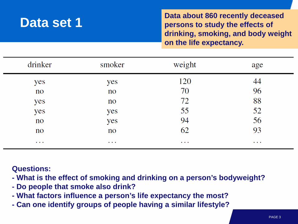
Data set 1
PAGE 3
Data about 860 recently deceased persons to study the effects of drinking, smoking, and body weight on the life expectancy.
Questions:- What is the effect of smoking and drinking on a person’s bodyweight?- Do people that smoke also drink?- What factors influence a person’s life expectancy the most?- Can one identify groups of people having a similar lifestyle?

Data set 2
PAGE 4
Data about 420 students to investigate relationships among course gradesand the student’s overall performance in the Bachelor program.
Questions:- Are the marks of certain courses highly correlated?- Which electives do excellent students (cum laude) take?- Which courses significantly delay the moment of graduation?- Why do students drop out?- Can one identify groups of students having a similar study behavior?

Data set 3
PAGE 5
Data on 240 customer orders in a coffee bar recorded by the cash register.
Questions:- Which products are frequently purchased together?- When do people buy a particular product?- Is it possible to characterize typical customer groups?- How to promote the sales of products with a higher margin?

Variables
• Data set (sample or table) consists of instances (individuals, entities, cases, objects, or records).
• Variables are often referred to as attributes, features, or data elements.
• Two types:− categorical variables: − ordinal (high-med-low, cum laude-passed-failed) or − nominal (true-false, red-pink-green)
− numerical variables (ordered, cannot be enumerated easily)
PAGE 6

Supervised Learning
• Labeled data, i.e., there is a response variable that labels each instance.
• Goal: explain response variable (dependent variable) in terms of predictor variables (independent variables).
• Classification techniques (e.g., decision tree learning) assume a categorical response variable and the goal is to classify instances based on the predictor variables.
• Regression techniques assume a numerical response variable. The goal is to find a function that fits the data with the least error.
PAGE 7

Unsupervised Learning
• Unsupervised learning assumes unlabeled data, i.e., the variables are not split into response and predictor variables.
• Examples: clustering (e.g., k-means clustering and agglomerative hierarchical clustering) and pattern discovery (association rules)
PAGE 8

Decision tree learning: data set 1
PAGE 9
smoker
young(195/11)
yes
drinker
weight
no
no
old(65/2)
yes
<90 ≥90
young(381/55)
old(219/34)

Decision tree learning: data set 2
PAGE 10
logic
failed(79/10)
- ≥8
passed(31/7)
failed(101/8)
linear algebra
programming
operat. research
cum laude(20/2)
<8
<6
<6
passed(82/7)
≥6
≥6
passed(87/11)
≥7
<7
linear algebra ≥6
<6
failed(20/4)

Decision tree learning: data set 3
PAGE 11
tea ≥1
latte
1
0
≥2 muffin(30/1)
no muffin(189/10)
muffin(4/0)
espresso
0
0
muffin(6/2)
≥1
no muffin(11/3)

Basic idea
• Split the set of instances in subsets such that the variation within each subset becomes smaller.
• Based on notion of entropy or similar.
• Minimize average entropy; maximize information gain per step.
PAGE 12
smoker
young(195/11)
yes
drinker
no
no
old(65/2)
yes
young(600/240)
#young=184#old=11
E = 0.313027
#young=360#old=240
E=0.970951
#young=2#old=63E=0.198234
Overall E = 0.763368
smoker
young(195/11)
yes no#young=184
#old=11E = 0.313027
Overall E = 0.839836
young(665/303)
#young=362#old=303E=0.994314
Overall E = 0.946848young(860/303)
#young=546#old=314
E=0.946848
split on attribute smoker
split on attribute drinker
information gain is 0.107012
information gain is 0.076468

Clustering
PAGE 13
age
weight
age
weight
+
+ +cluster A cluster B
cluster C

k-means clustering
PAGE 14
+++ +
+
+
(a) (b) (c)

Agglomerative hierarchical clustering
PAGE 15
a
b
c
d
e
f
g
h
i j
a b c d e f g h i j
ab cd fg hi
hijefg
abcdefghij
abcdefghij
(a) (b)
dendrogram

Levels introduced by agglomerative hierarchical clustering
PAGE 16
a
b
c
d
e
f
g
h
i j
a b c d e f g h i j
ab cd fg hi
hijefg
abcdefghij
abcdefghij
(a) (b)
Any horizontal line in dendrogram corresponds to a concrete clustering at a particular level of abstraction

Association rule learning
• Rules of form “IF X THEN Y”
PAGE 17

Special case: market basket analysis
PAGE 18

Example(people that order tea and latte also order muffins)
• Support should be as high as possible (but will be low in case of many items).• Confidence should be close to 1.• High lift values suggest a positive correlation (1 if independent).
PAGE 19

Brute force algorithm
PAGE 20

Apriori (optimization based on two observations)
PAGE 21

Sequence mining
PAGE 22

Episode mining(32 time windows of length 5)
PAGE 23
10 11 12 13 14 15 16 17 18 19 20 21 22 23 24 25 26 27 28 29 30 31 32 33 34 35 36 37
a c b de c b b cf a e eb c d c b
a
b
c
d
E1
b
c
E2
a
b
c
d
E3

Occurrences
PAGE 24
a
b
c
d
E1
b
c
E2
a
b
c
d
E3
10 11 12 13 14 15 16 17 18 19 20 21 22 23 24 25 26 27 28 29 30 31 32 33 34 35 36 37
a c b de c b b cf a e eb c d c b
E1
E2 (16x)
E1 E3

Hidden Markov models
• Given an observation sequence, how to compute the probability of the sequence given a hidden Markov model?
• Given an observation sequence and a hidden Markov model, how to compute the most likely “hidden path” in the model?
• Given a set of observation sequences, how to derive the hidden Markov model that maximizes the probability of producing these sequences?
PAGE 25
s1 s2 s3
0.70.3
0.2
0.8
a b c d e
0.5 0.5 0.40.6 0.8 0.2
1.0
s state
transition with probability0.7
x observation
0.5 observation probability

Relation between data mining and process mining
• Process mining: about end-to-end processes.• Data mining: data-centric and not process-centric.• Judging the quality of data mining and process
mining: many similarities, but also some differences.• Clearly, process mining techniques can benefit from
experiences in the data mining field.• Let us now focus on the quality of mining results.
PAGE 26
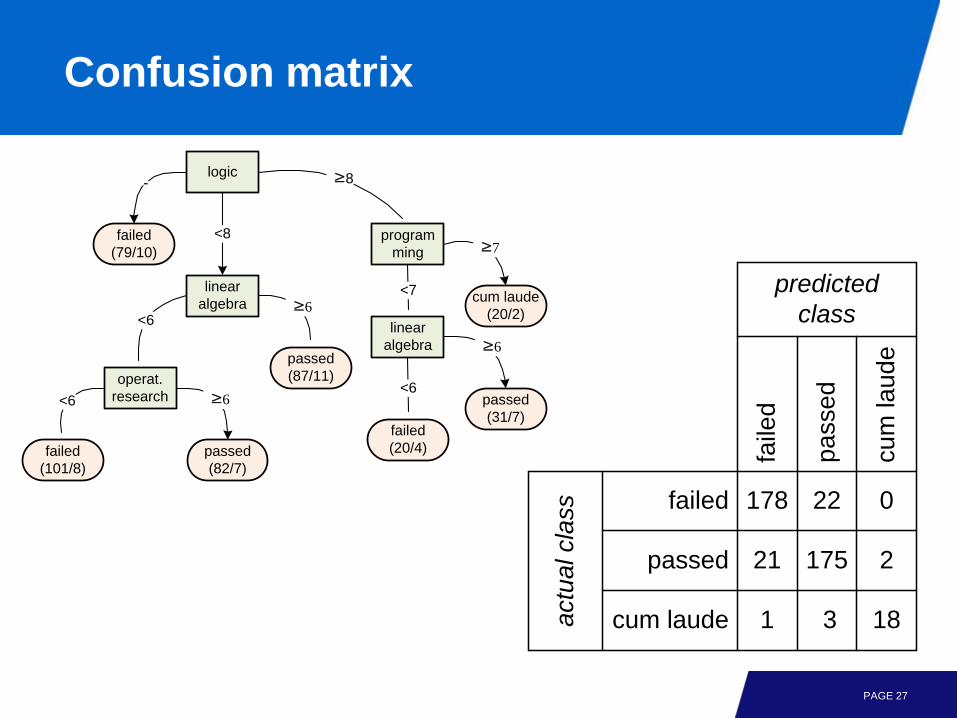
Confusion matrix
PAGE 27
failed
passed
cum laude
faile
d
pass
ed
cum
laud
e
178 22 0
217521
1 3 18
predicted class
actu
al c
lass
logic
failed(79/10)
- ≥8
passed(31/7)
failed(101/8)
linear algebra
programming
operat. research
cum laude(20/2)
<8
<6
<6
passed(82/7)
≥6
≥6
passed(87/11)
≥7
<7
linear algebra ≥6
<6
failed(20/4)

Confusion matrix: metrics
PAGE 28
+ tp fn
tnfp
predicted class
actu
al
clas
s
-
+ -p
n
p’ n’ N
name
error
accuracy
formula
(fp+fn)/N
tp-rate
fp-rate
precision
recall
(tp+tn)/Ntp/pfp/ntp/p’tp/p
(a) (b)
tp is the number of true positives, i.e., instances that are correctly classified as positive.fn is the number of false negatives, i.e., instances that are predicted to be negative but should have been classified as positive.fp is the number of false positives, i.e., instances that are predicted to be positive but should have been classified as negative.tn is the number of true negatives, i.e., instances that are correctly classified as negative.

Example
PAGE 29
smoker
young(195/11)
yes
drinker
no
no
old(65/2)
yes
young(600/240)
#young=184#old=11
E = 0.313027
#young=360#old=240
E=0.970951
#young=2#old=63E=0.198234
Overall E = 0.763368
smoker
young(195/11)
yes no#young=184
#old=11E = 0.313027
Overall E = 0.839836
young(665/303)
#young=362#old=303E=0.994314
Overall E = 0.946848young(860/303)
#young=546#old=314
E=0.946848
split on attribute smoker
split on attribute drinker
information gain is 0.107012
information gain is 0.076468
young
old
youn
g
old
546 0
0314
predicted class
actu
al
clas
s young
old
youn
g
old
544 2
63251
predicted class
actu
al
clas
s
(a) (b)

Cross-validation
PAGE 30
data set
test set
learning algorithm
test
model
split
performanceindicator
training set

k-fold cross-validation
PAGE 31
data set
k data sets
split
rotate
learning algorithm
test
model
performanceindicator

Occam’s Razor
• Principle attributed to the 14thcentury English logician William of Ockham.
• The principle states that “one should not increase, beyond what is necessary, the number of entities required to explain anything”, i.e., one should look for the “simplest model” that can explain what is observed in the data set.
• The Minimal Description Length (MDL) principle tries to operationalize Occam’s. In MDL performance is judged on the training data alone and not measured against new, unseen instances. The basic idea is that the “best” model is the one that minimizes the encoding of both model and data set.
PAGE 32