Chapter 3 -...
79
Chapter 3 Examining Relationships
Transcript of Chapter 3 -...

Chapter 3
Examining Relationships

Lesson 3-1
Scatterplots

Variables
Response variable (dependent)
Measures the outcome of a study.
Explanatory variable (independent)
Attempts to explain the observed outcomes
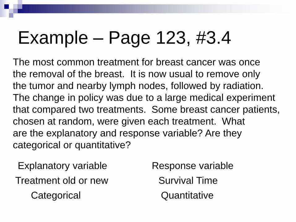
Example – Page 123, #3.4
The most common treatment for breast cancer was once
the removal of the breast. It is now usual to remove only
the tumor and nearby lymph nodes, followed by radiation.
The change in policy was due to a large medical experiment
that compared two treatments. Some breast cancer patients,
chosen at random, were given each treatment. What
are the explanatory and response variable? Are they
categorical or quantitative?
Explanatory variable Response variable
Treatment old or new
Categorical
Survival Time
Quantitative

Scatterplot
A scatterplot shows the relationship between two
quantitative variables measured on the same individuals.
Always plot the explanatory variable (if there is one) on the
horizontal axis (x-axis) of a scatterplot. The response
variable on the vertical axis (y-axis).
If there is no explanatory-response distinction, either
variable can go on the horizontal axis.
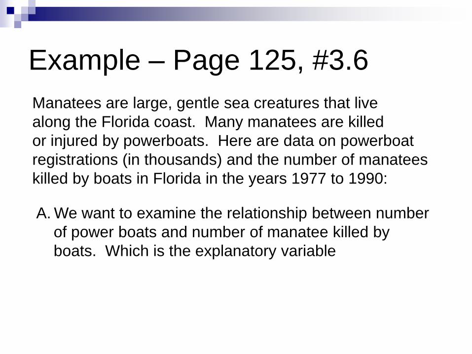
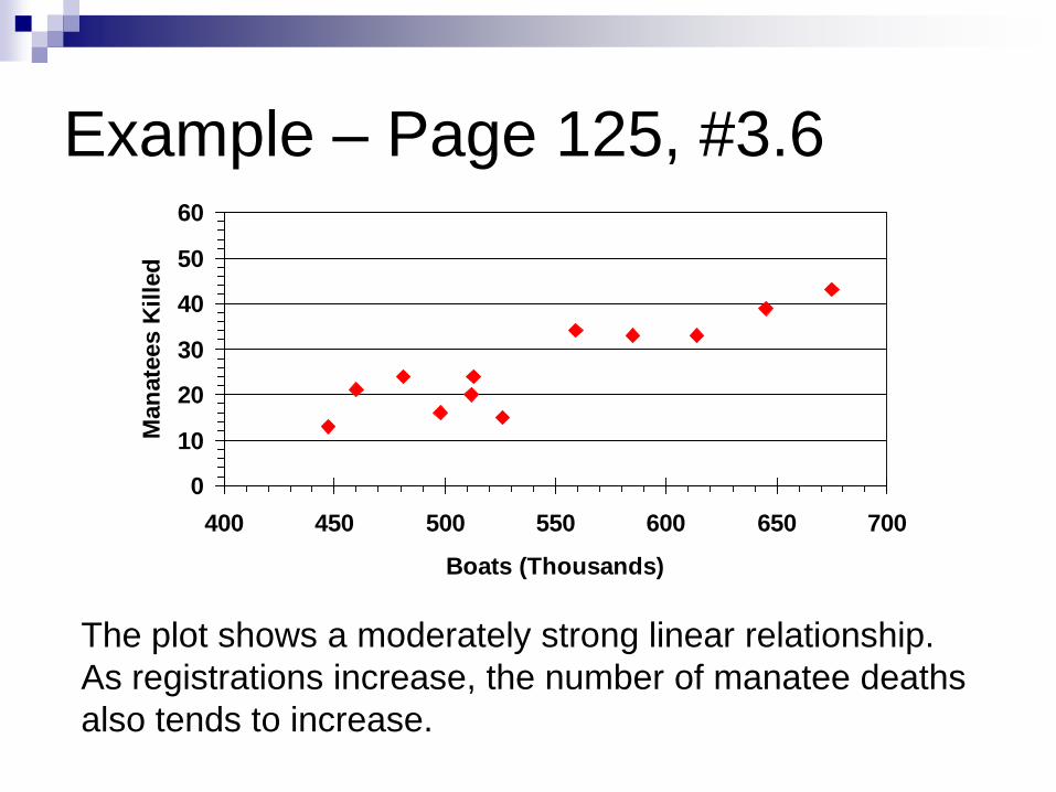
Example – Page 125, #3.6
Manatees are large, gentle sea creatures that live
along the Florida coast. Many manatees are killed
or injured by powerboats. Here are data on powerboat
registrations (in thousands) and the number of manatees
killed by boats in Florida in the years 1977 to 1990:
A. We want to examine the relationship between number
of power boats and number of manatee killed by
boats. Which is the explanatory variable
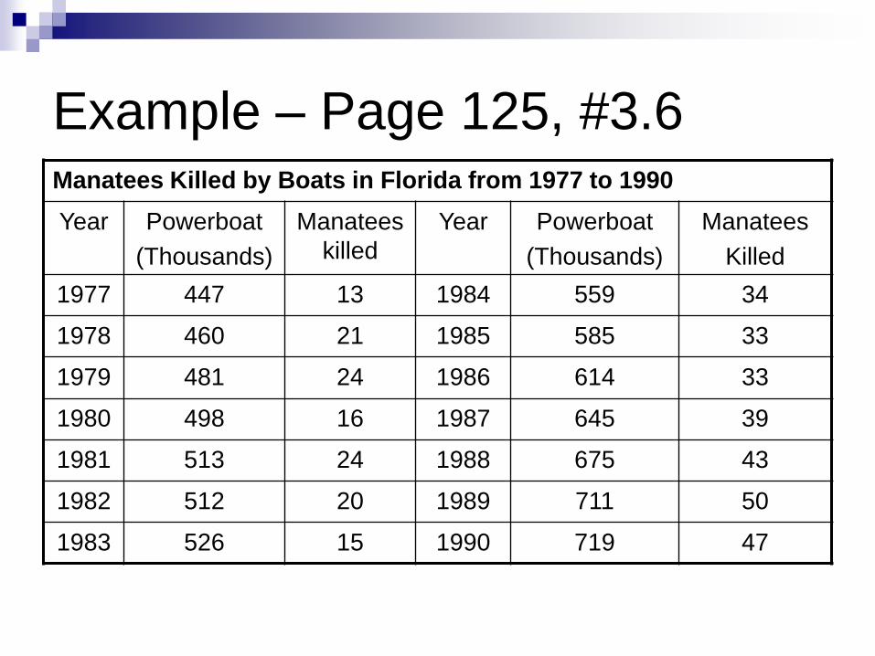
Example – Page 125, #3.6Manatees Killed by Boats in Florida from 1977 to 1990
Year Powerboat
(Thousands)
Manatees
killed
Year Powerboat
(Thousands)
Manatees
Killed
1977 447 13 1984 559 34
1978 460 21 1985 585 33
1979 481 24 1986 614 33
1980 498 16 1987 645 39
1981 513 24 1988 675 43
1982 512 20 1989 711 50
1983 526 15 1990 719 47

Example – Page 125, #3.6
A. We want to examine the relationship between number
of power boats and number of manatee killed by
boats. Which is the explanatory variable
Explanatory Variable = Number of powerboat registrations
B. Make a scatterplot of these data. (Be sure to label the
axes with variable names, not just x and y.) What does
the scatterplot show about the relationship between these
variables?

Example – Page 125, #3.6Manatees Killed by Boats in Florida from 1977 to 1990
Year Powerboat
(Thousands)
Manatees
killed
Year Powerboat
(Thousands)
Manatees
Killed
1977 447 13 1984 559 34
1978 460 21 1985 585 33
1979 481 24 1986 614 33
1980 498 16 1987 645 39
1981 513 24 1988 675 43
1982 512 20 1989 711 50
1983 526 15 1990 719 47

Example – Page 125, #3.6
2nd Y=
ZOOMSTAT
Example – Page 125, #3.6
0
10
20
30
40
50
60
400 450 500 550 600 650 700
Boats (Thousands)
Man
ate
es K
ille
d
The plot shows a moderately strong linear relationship.
As registrations increase, the number of manatee deaths
also tends to increase.
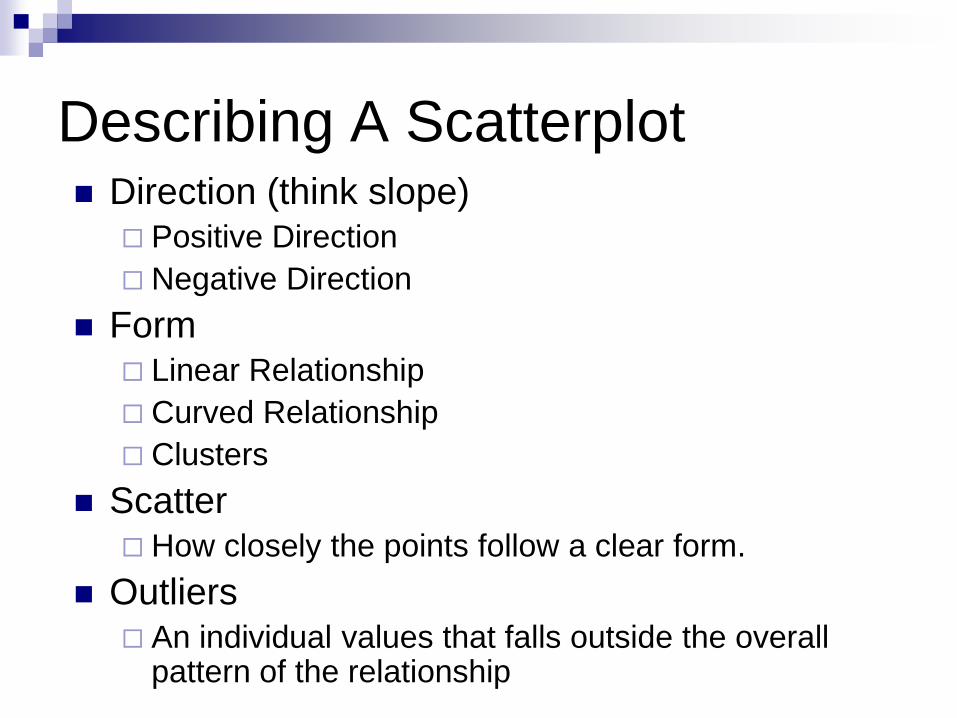
Describing A Scatterplot Direction (think slope)
Positive Direction
Negative Direction
Form Linear Relationship
Curved Relationship
Clusters
Scatter How closely the points follow a clear form.
Outliers An individual values that falls outside the overall
pattern of the relationship

Example – Page 129, #3.9Use the scatterplot from Exercise 3.6 (Page 125). You
make a scatterplot of power boats registered in Florida
and manatees killed by boats.
A. Describe the direction of the relationship. Are the
variables positively or negatively associated?
B. Describe the form of the association. Is it linear?
C. Describe the strength of the relationship. Can the number
of manatees killed be predicted accurately from powerboat
registrations? If powerboat registrations remained constant
at 719,000, about how many manatees would be killed by
boats each year?

Example – Page 129, #3.9
A. Describe the direction of the relationship. Are the
variables positively or negatively associated?
The variables are positively associated; that is, at the
number of jet skis in use increases, the number of
manatees killed also increase.
B. Describe the form of the association. Is it linear?
The association is moderately linear.
Example – Page 129, #3.9
C. Describe the strength of the relationship. Can the number
of manatees killed be predicted accurately from powerboat
registrations? If powerboat registrations remained constant
at 719,000, about how many manatees would be killed by
boats each year?
The association is relatively strong. The number of manatees
killed can be predicted accurately from the number of
powerboat registrations. If the number of registrations remains
constant 719,000, we would expect between 45 and 50
manatees to be killed per year.

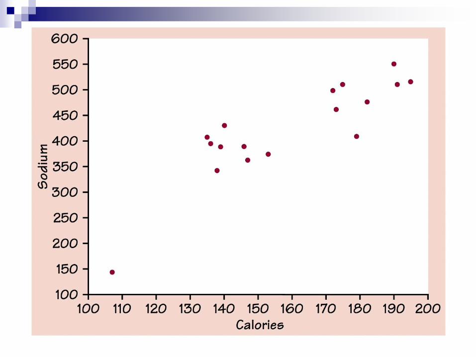
Example – Page 136, #3.16
Calories and hot dogs that are high in calories are also high
in salt? The following slide is a scatterplot of the calories
and salt content (measured as milligrams of sodium) in
17 brands of meat hot dogs.
Example – Page 136, #3.16
A. Roughly what are the lowest and highest calories counts
among these brands? Roughly what is the sodium level in
the brands with the fewest and with the most calories.
B. Does the scatterplot show a clear positive or negative
association? Say in words what this association means
about calories and salt in hot dogs.
C. Are there any outliers? is the relationship (ignoring outliers)
roughly linear in form? Still ignoring outliers, how strong
would say the relationship between calories and sodium is?
Example
Example – Page 136, 3.16
A. Lowest: about 107 calories with about 145 mg of sodium
Highest: about 195 calories with about 510 mg of sodium
B. There is positive association: high calorie hot dogs tend
to be high in salt, and low calorie hot dogs tend to have
low sodium.
C. The lower left point is an outlier. Ignoring the point,
the remaining points seem to fall roughly on a line.
The relationship is moderately strong.

Lesson 3-2
Correlation

Correlation
Correlation measures the direction and strength of the linear
relationship between two quantitative variables.
Correlation is usually written as r.
1
1i i
x y
x x y xr
n s s

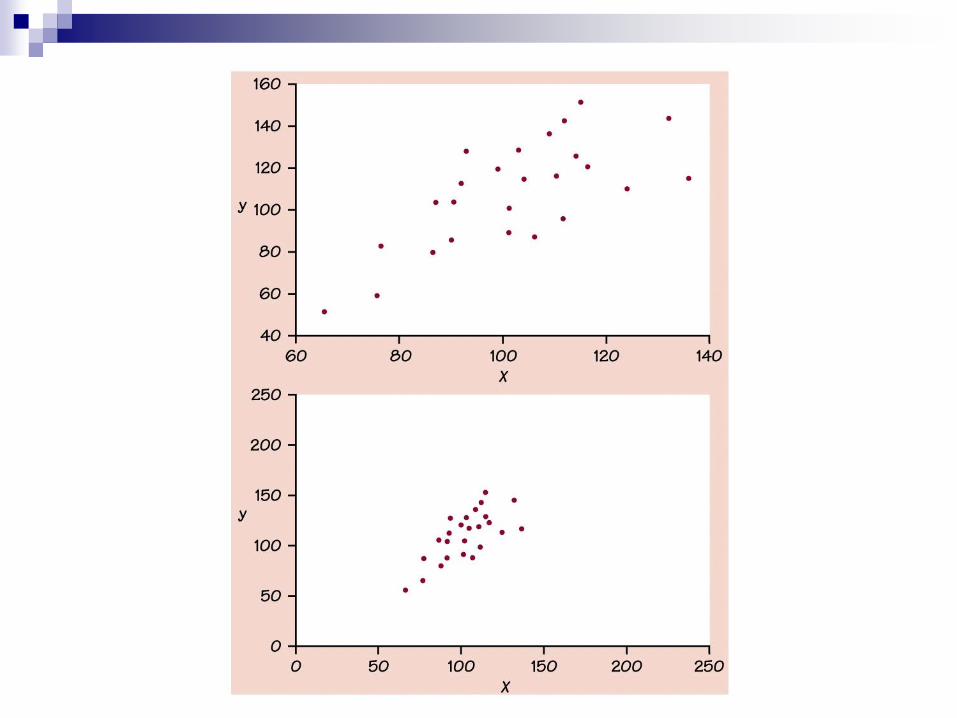
Example – Page 142, #3.24
Classifying Fossils. Exercise 3.19 (Page 138) gives the
lengths of two bones in five fossil specimens of extinct
beast Archaeopteryx.
: 38 56 59 64 74
: 41 63 70 72 84
Femur
Humerus
A. Find the correlation r step-by-step. That is find the mean
and standard deviation of the femur lengths and of the
humerus lengths. Then find the five standardized values
for each variable and use the formula for r.

Example – Page 142, #3.24
38 41 1.53 1.573 2.4079
56 63 0.1667 0.1888 0.03147
59 70 0.0601 0.25173 0.01526
64 72 0.43944 0.37759 0.16593
74 84 1.1971 1.1328 1.356
3.976594
i i i i
x y x y
x x y y x x y yx y
s s s s
58.2x 13.1985xs 66y 15.89025ys
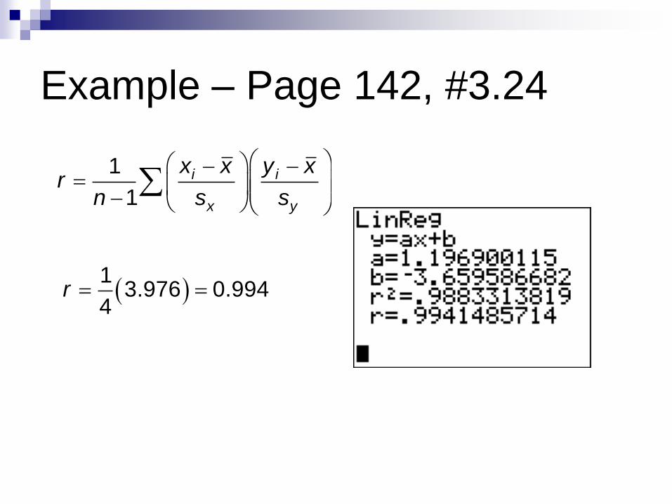
Example – Page 142, #3.24
1
1i i
x y
x x y xr
n s s
1
3.976 0.9944
r
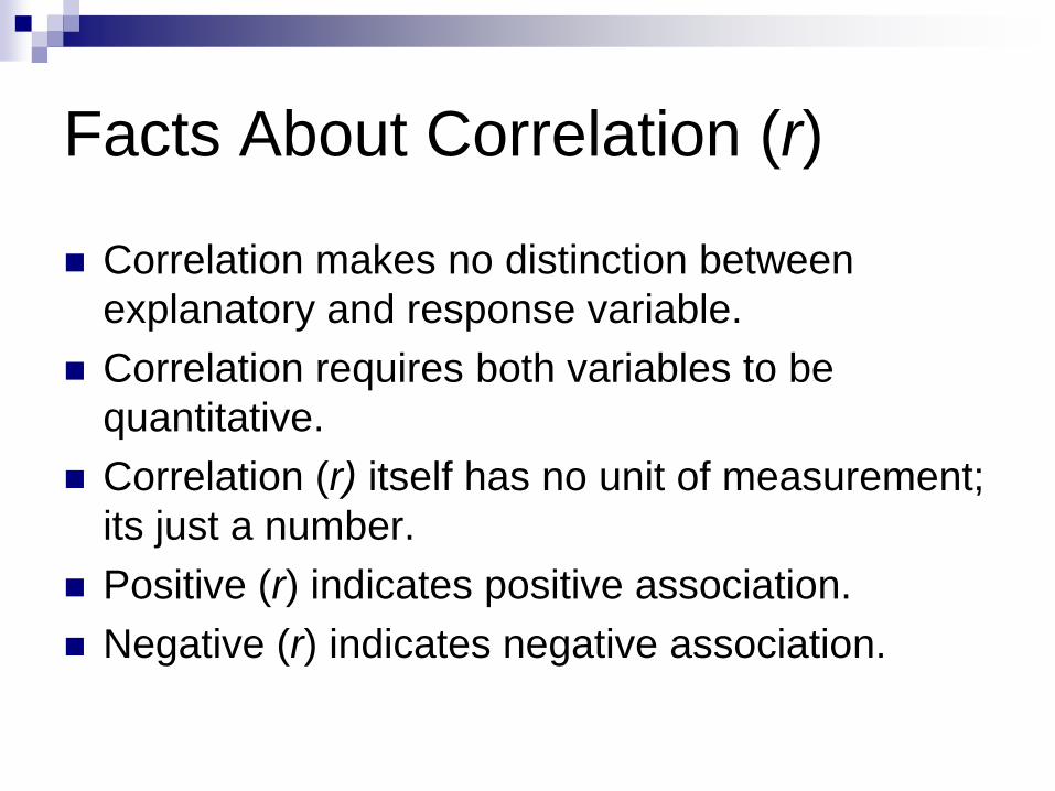
Facts About Correlation (r)
Correlation makes no distinction between
explanatory and response variable.
Correlation requires both variables to be
quantitative.
Correlation (r) itself has no unit of measurement;
its just a number.
Positive (r) indicates positive association.
Negative (r) indicates negative association.

Facts About Correlation (r)
The correlation (r) is always between -1 and 1.
The closer (r) is to +1, the stronger the evidence of positive association between two variables.
The closer (r) is to -1, the stronger the evidence of negative association between to variables.
If (r) is close to 0, does not rule out any strong relationship between x and y, there could still be a strong relationship but one that is not linear.
Correlation is strongly effected by a outlying observations.

Positive Linear Correlation
Perfect Positive
Linear Correlation
Strong Positive
Linear Correlation
1r 0.9r
Weak Positive
Linear Correlation
0.4r
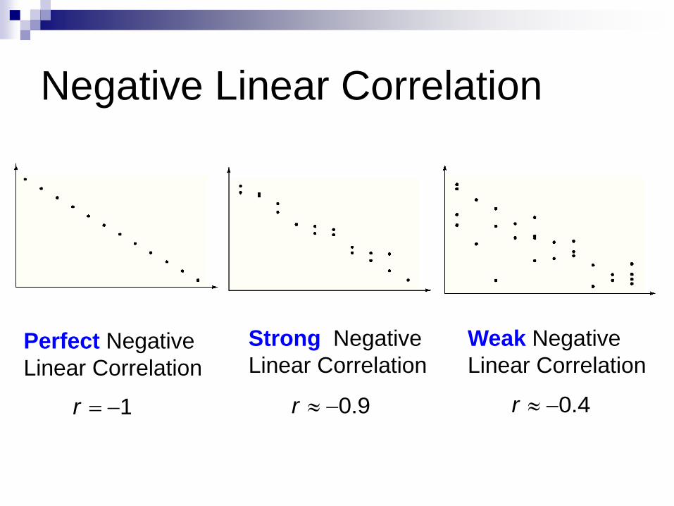
Negative Linear Correlation
Perfect Negative
Linear Correlation
Strong Negative
Linear Correlation
1r 0.9r
Weak Negative
Linear Correlation
0.4r
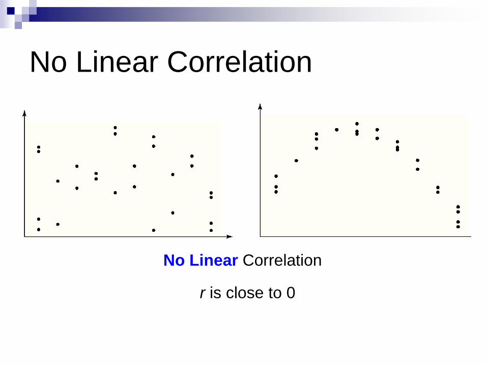
No Linear Correlation
No Linear Correlation
r is close to 0
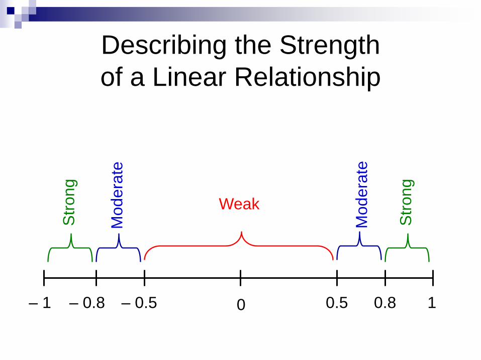
Describing the Strength
of a Linear Relationship
0 10.80.5– 1 – 0.8 – 0.5
Str
ong
Str
ong
Modera
te
Mo
dera
te
Weak

Example – Page 149, #3.32Do people with larger brains have higher IQ scores? A
study looked at 40 volunteer subjects, 20 men and 20
women. Brain size was measured by magnetic resonance
imagining. Table 3-3 gives the data. the MRI count is the
number of “pixels” the brain covered in the image. IQ was
measured by the Wechsler test.
A) Make a scatterplot of IQ score versus MRI count, using
distinct symbols for the mean and women. In addition
find the correlation between IQ and MRI for all 40 subjects
for the men alone and for the women alone.

Example – Page 149, #3.32

Example – Page 149, #3.32
0 3576
0 4984
0 3257
.
.
.
all
men
women
r
r
r

Example – Page 149, #3.32
B) Men are larger than women on the average, so they
have larger brains. How is this size effect visible in your
plot? Find the mean MRI count for men and women to verify
the difference.
954 855
862 655
,
,
men
women
x
x
The points for men are
generally located on the right
side of the plot , while the women’s
points are generally on the left.
Example – Page 149, #3.32C) Your result in (b) suggests separating men and women in
looking at he relationship between brain size and IQ.
Use your work in (a) to comment on the nature and
strength of this relationship for women and for men.

Example – Page 149, #3.32
The correlation for men and women suggests that there is
a moderately positive association for men and a weak one
for women. However, one significant feature of the data
that can be observed in the scatterplot is that the sample
group was highly stratified; that is, there were 10 men and
10 women with high IQs (at least 130), while other 10 of
each gender had IQs of no more than 103. The men’s
higher correlation can be attributed partly to the two
subjects with large brains and 103 IQs (which are relative
to the low IQ group). The men’s correlation might not
remain so high with a larger sample.

Lesson 3-3
Line of Best Fit

Best Fit Line
Is a straight line (equation) that describes how a response variable y changes as an explanatory variable x changes.
A best Fit Line (equation) is used to predict the value of y for a given value of x.
Best Fit Line unlike correlation, requires that we have an explanatory variable and a response variable.
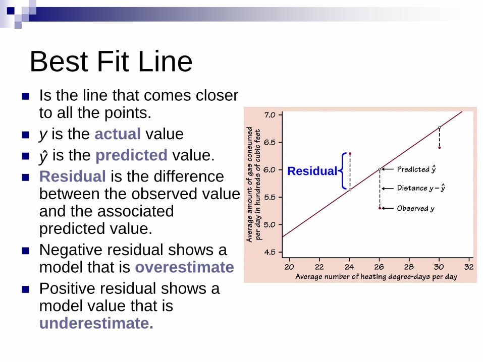
Best Fit Line Is the line that comes closer
to all the points.
y is the actual value
is the predicted value.
Residual is the difference between the observed value and the associated predicted value.
Negative residual shows a model that is overestimate
Positive residual shows a model value that is underestimate.
Residualy

“Best Fit” Means Least-Squares
The line of “Best Fit” is
the line for which the
sum of the squared
residuals is the smallest.
The line of “Best Fit” is
called a Least-squares
Regression Line
(LSRL)

Equation of LSRL
The line must go through the point
Equation
Slope
Intercept
0 1y b b x
1
y
x
sb r
s
0 1b y b x
,x y
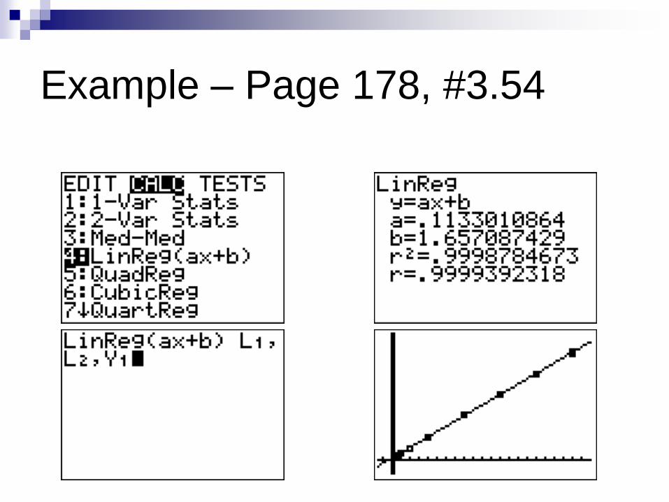
Example – Page 178, #3.54
Keeping water supplies clean requires regular measurement
of levels of pollutants. The measurements are indirect – a
typical analysis involves forming a dye by a chemical
reaction with the dissolved pollutant, then passing light
through the solution and measuring its “absorbance.”
To calibrate such measurements, the laboratory measures
known standard solutions and uses regression to relate
series of data on the absorbance for different levels of
nitrates. Nitrates are measured in milligrams per liter of water
Example – Page 178, #3.54
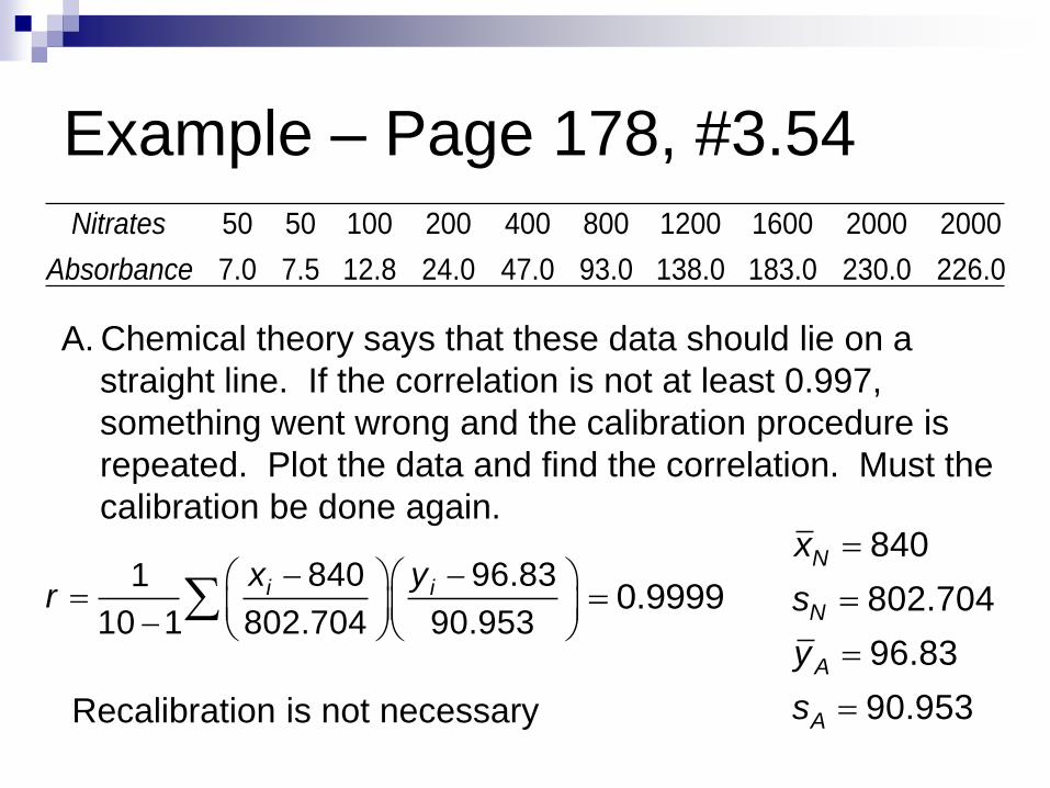
50 50 100 200 400 800 1200 1600 2000 2000
7.0 7.5 12.8 24.0 47.0 93.0 138.0 183.0 230.0 226.0
Nitrates
Absorbance
A. Chemical theory says that these data should lie on a
straight line. If the correlation is not at least 0.997,
something went wrong and the calibration procedure is
repeated. Plot the data and find the correlation. Must the
calibration be done again.840
802.704
96.83
90.953
N
N
A
A
x
s
y
s
0.9999
Recalibration is not necessary
840 96.831
10 1 802.704 90.953i ix y
r

Example – Page 178, #3.54
B. What is the equation of the least-square lines for
predicating absorbance from concentration? If the lab
analyzed a specimen with 500 milligrams of nitrates per
liter, what do you expect the absorbance to be? Based
on your plot and the correlation, do you expect your
predicted absorbance to be very accurate?
840
802.704
96.83
90.953
N
N
A
A
x
s
y
s
0.9999r
1
90.953(0.9999) 0.1133
802.704
y
x
sb r
s
0 1
0
0
96.83 (0.1133)(840)
1.658
b y b x
b
b
ˆ 1.658 0.1133y x

Example – Page 178, #3.54
ˆ 1.658 0.1133y x
500
ˆ 1.658 0.1133(500)
58.31
x
y
This prediction should be
very accurate since the
relationship is so strong
Example – Page 178, #3.54
Lesson 3-3
The Role of r2 in Regression
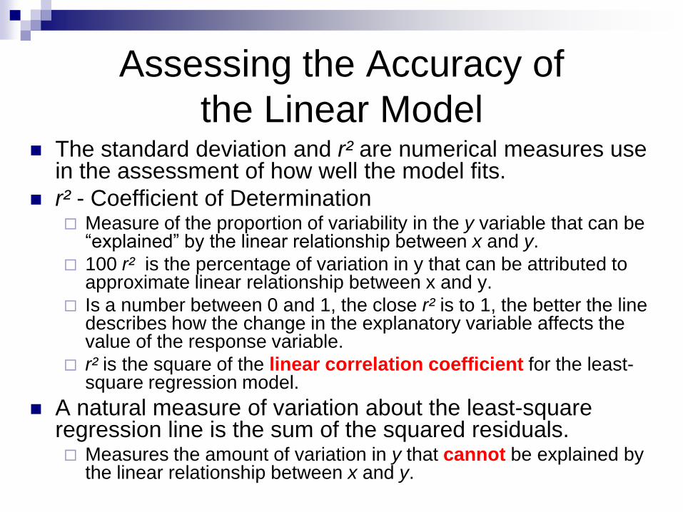
Assessing the Accuracy of
the Linear Model The standard deviation and r² are numerical measures use
in the assessment of how well the model fits.
r² - Coefficient of Determination Measure of the proportion of variability in the y variable that can be
“explained” by the linear relationship between x and y.
100 r² is the percentage of variation in y that can be attributed to approximate linear relationship between x and y.
Is a number between 0 and 1, the close r² is to 1, the better the line describes how the change in the explanatory variable affects the value of the response variable.
r² is the square of the linear correlation coefficient for the least-square regression model.
A natural measure of variation about the least-square regression line is the sum of the squared residuals. Measures the amount of variation in y that cannot be explained by
the linear relationship between x and y.
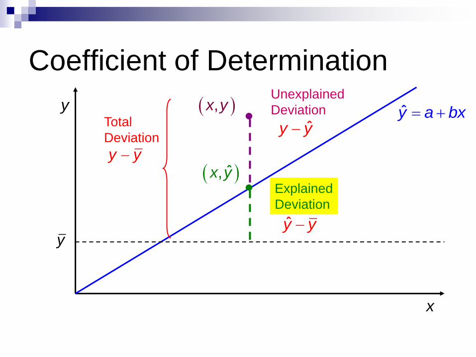
Coefficient of Determination
y
x
Total
Deviation
y y
,x y
ˆ,x y
Unexplained
Deviation y a bx ˆy y
Explained
Deviation
y y
y

Coefficient of Determination
r² =Explained Variation
Total Variation
= 1 –Total Variation
Unexplained Variation
22
2
2
ˆy y y ySST SSEr
SST y y
Total Unexplained
Total

Example – Page 165, #3.42
A study of class attendance and grades among first
year students at a state university showed that in
general students who attended a higher percent
of their classes earned higher grades. Class attendance
explained 16% of the variation in grade index among
students. What is the numerical value of the correlation
between percent of classes attended and grade index?
2 0.16r
2 0.16
0.40
r
r
Higher attendance goes with
high grades, so the correlation
must be positive

Example – Page 166, #3.44
Some people think that the behavior of the stock
market in January predicts its behavior for the rest of
the year. Take the explanatory variable x to be the
percent change in a stock market index January and the
response variable y to be the change in the index for
the entire year. We expect a positive correlation between
x and y because the change in January contributes to
the full year’s change. Calculation from data for the years
1960 to 1997 gives
1.75%
9.07%
x
y
5.36%xs
15.35%ys
0.596r
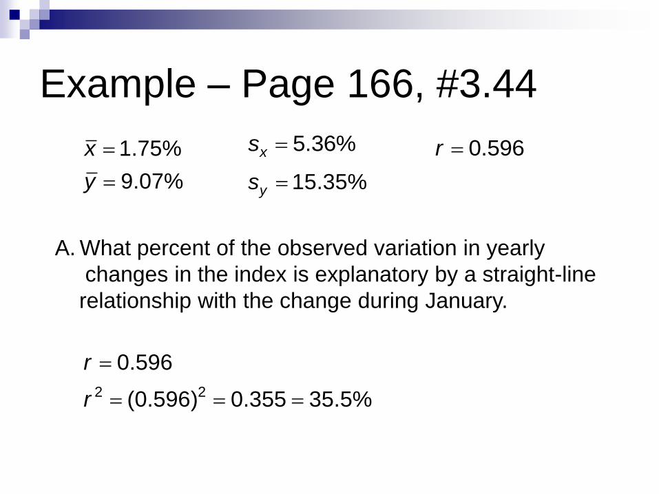
Example – Page 166, #3.44
1.75%
9.07%
x
y
5.36%xs
15.35%ys
0.596r
A. What percent of the observed variation in yearly
changes in the index is explanatory by a straight-line
relationship with the change during January.
2 2
0.596
(0.596) 0.355 35.5%
r
r

Example – Page 166, #3.44
1.75%
9.07%
x
y
5.36%xs
15.35%ys
0.596r
B. What is the equation of the least-squares line for
predicting full-year change from January change?
1
0.1535(0.596) 1.707
.0536
y
x
sb r
s
0 1
0
0
.0907 (1.707)(.0175)
0.06083 6.083%
b y b x
b
bˆ 6.083% 1.707y x
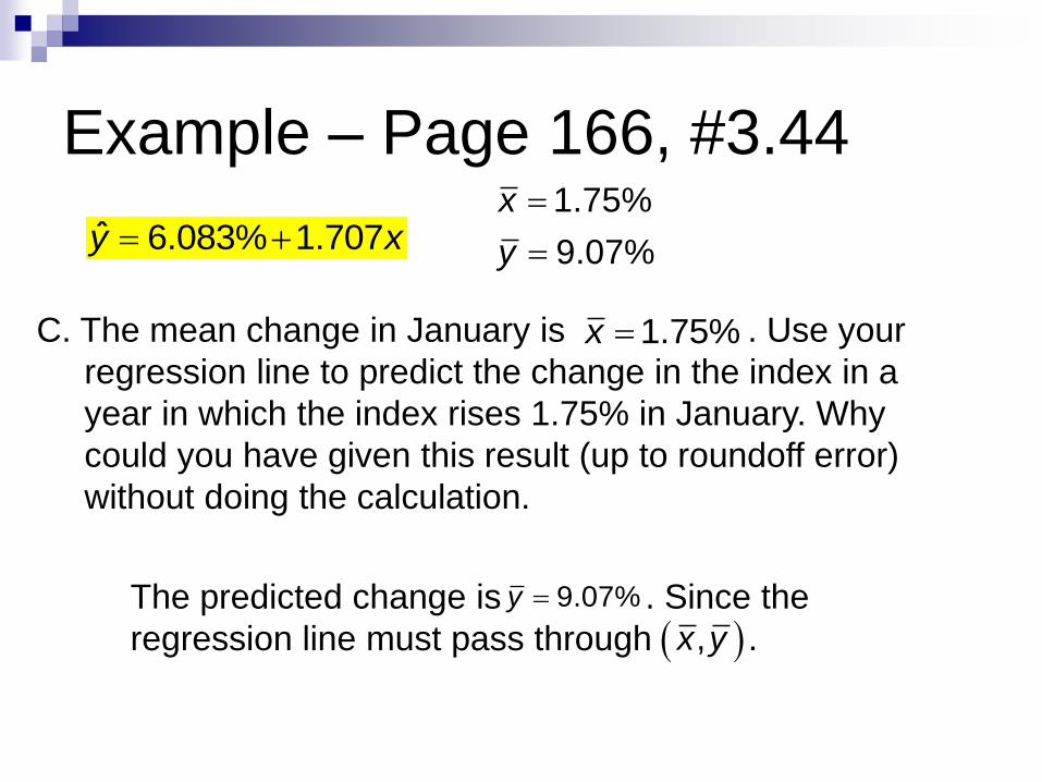
Example – Page 166, #3.441.75%
9.07%
x
y
C. The mean change in January is . Use your
regression line to predict the change in the index in a
year in which the index rises 1.75% in January. Why
could you have given this result (up to roundoff error)
without doing the calculation.
ˆ 6.083% 1.707y x
1.75%x
The predicted change is . Since the
regression line must pass through .
9.07%y
,x y

Assumptions and Conditions
Check the scatterplot. The shape must be linear or we can’t use regression
at all.
Watch out for outliers.Outlying values have large residuals and squaring
makes their influences that much greater.
Outlying points can dramatically change a regression model. They can change the sign of the slope, misleading us about
the underlying relationship between variables.
A r² of 100% You may have accidentally regressed two variables
that measure the same thing.

Lesson 3-3
Residual Plot

Assumptions and Conditions Don’t extrapolate beyond the data.
A linear model will often do reasonable job of
summarizing a relationship in the narrow range of
observed x-values.
Beware of predicting y-values for x-values that lie
outside the range of the original data.
If you must extrapolate into the future, at least don’t
believe that the prediction will come true!
Don’t infer that x causes y just because there is
good linear model for their relationship.

Residuals
A residuals is the difference between an
observed value of the response variable and the
value predicted by the regression line.
Unexplained Deviation
Plotting the residual
A residual plot is a scatterplot of the (x, residual)
pairs
Residual plot is a good place to start when
assessing the appropriateness of the regression
line.

Residual Plot
Determine whether a linear model is appropriate to describe the relationship between the explanatory and response variables.
Residual are what is “left over” after the model describes the relationship, they often reveal subtleties that were not clear from a plot of the original data.
Determine whether the variance of the residuals is constant.
Check for outliers

Residual Plots – Uniformed
The uniform scatter of points indicated that the regression
line is good model

Residual Plots – Curved
The residuals have a curved pattern, so a straight line
is an inappropriate model

Residual Plots – Increasing/Decreasing
The response variable y has more spread for larger values
of the explanatory variable x, so prediction will be less
accurate when x is large.
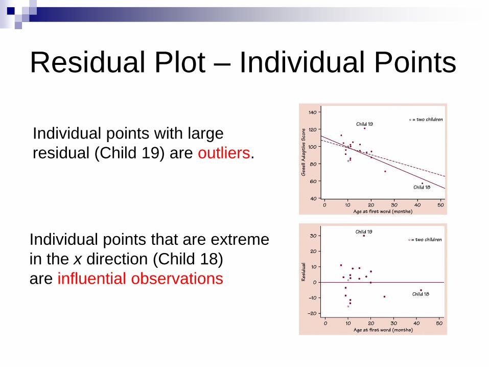
Residual Plot – Individual Points
Individual points with large
residual (Child 19) are outliers.
Individual points that are extreme
in the x direction (Child 18)
are influential observations

Influential Observations
An outlier is an observation that lies outside the overall
pattern of the other observation.
An observation is influential for a statistical calculation
if removing it would markedly change the result of the
calculation.
Points that are outliers in the x directions of a scatterplot
are often influential for the least-square regression line.

Case 1
(outlier)
Case 2
Case 3
(influential)
Influential observations typically exist when
the point is large relative to its x value.

Example – Page 175, #3.49
Lean body mass as a predictor of metabolic rate. Exercise
3.12, page 132 provides data from a study of dieting for
12 women and 7 men subjects. We explore the data
further.
A. Define two lists on your calculator, (L1) MASSF for
female mass and (L2) METF for female metabolic
rate. Define plots using the plotting symbol, and
plot the scatterplot.

Example – Page 175, #3.49

Example – Page 175, #3.49

Example – Page 175, #3.49
B. Perform least-squares regression on your calculator and
record the equation and the correlation. Lean body mass
explains what percent of the variation in metabolic rate
for women?
ˆ 201.1616 24.026y x
2
.8765
0.7682 76.8%
r
r
Lean body mass explains about 76.82% of the variation
in metabolic rate.
Example – Page 175, #3.49
C. Does the least-square line provide an adequate model
for the data? Define Plot2 to be a residual plot on your
calculator with residuals on the vertical axis and the
lean body mass (x-values) on the horizontal axis. Use
the plotting symbol.

Example – Page 175, #3.49
Graphing Residuals
Y1 → Vars/Y-Vars/Function
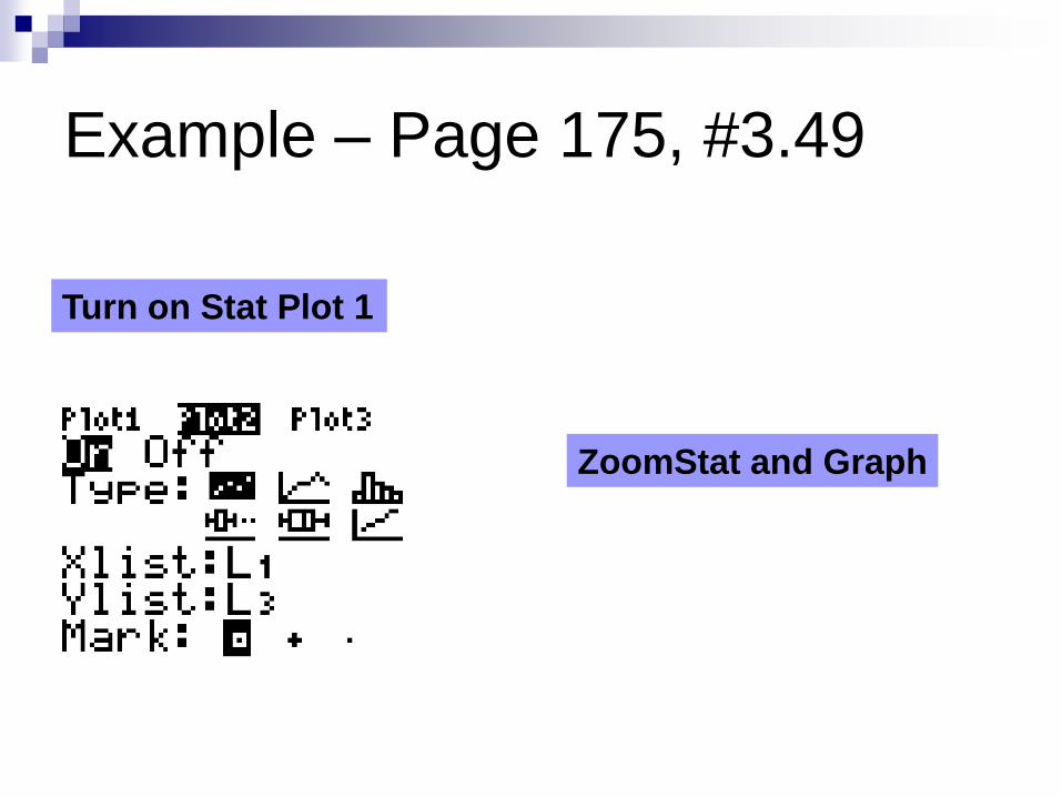
Example – Page 175, #3.49
Turn on Stat Plot 1
ZoomStat and Graph

Example – Page 175, #3.49

Example – Page 175, #3.49
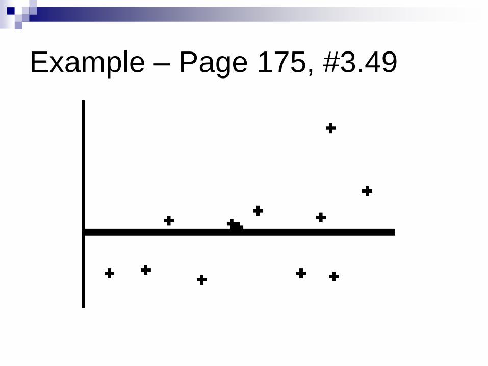
C. From the residual plot, the line does appear to provide
an adequate model. The residual are scattered about
the horizontal axis and no patterns are evident.
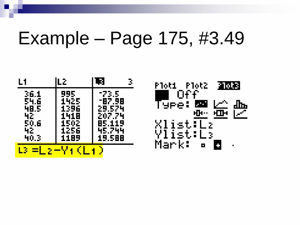
D. Define L3 to be the predicated y-values: define PLOT3
to be a residual plot on your calculator with residuals
on the vertical axis and predicted metabolic rate on
the horizontal axis. Use the + plotting symbol.
Example – Page 175, #3.49
Example – Page 175, #3.49

Example – Page 175, #3.49
D.The plots are identical in terms of the relative positions
of the data points.