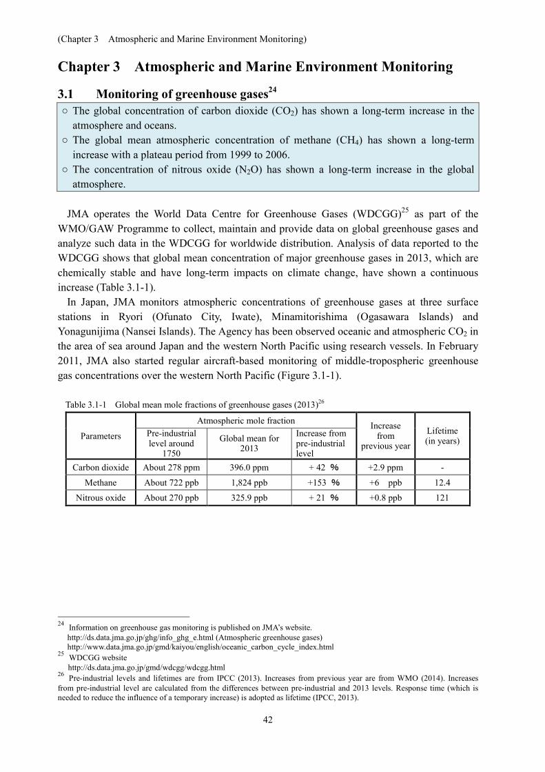
(Chapter 3 Atmospheric and Marine Environment Monitoring)

42

Chapter 3 Atmospheric and Marine Environment Monitoring

3.1 Monitoring of greenhouse gases24 ○ The global concentration of carbon dioxide (CO2) has shown a long-term increase in the

atmosphere and oceans. ○ The global mean atmospheric concentration of methane (CH4) has shown a long-term

increase with a plateau period from 1999 to 2006. ○ The concentration of nitrous oxide (N2O) has shown a long-term increase in the global

atmosphere. JMA operates the World Data Centre for Greenhouse Gases (WDCGG)25 as part of the

WMO/GAW Programme to collect, maintain and provide data on global greenhouse gases and analyze such data in the WDCGG for worldwide distribution. Analysis of data reported to the WDCGG shows that global mean concentration of major greenhouse gases in 2013, which are chemically stable and have long-term impacts on climate change, have shown a continuous increase (Table 3.1-1).

In Japan, JMA monitors atmospheric concentrations of greenhouse gases at three surface stations in Ryori (Ofunato City, Iwate), Minamitorishima (Ogasawara Islands) and Yonagunijima (Nansei Islands). The Agency has been observed oceanic and atmospheric CO2 in the area of sea around Japan and the western North Pacific using research vessels. In February 2011, JMA also started regular aircraft-based monitoring of middle-tropospheric greenhouse gas concentrations over the western North Pacific (Figure 3.1-1).

Table 3.1-1 Global mean mole fractions of greenhouse gases (2013)26

Parameters

Atmospheric mole fraction Increase from

previous year

Lifetime (in years)

Pre-industrial level around

1750

Global mean for 2013

Increase from pre-industrial level

Carbon dioxide About 278 ppm 396.0 ppm + 42 ％ +2.9 ppm -

Methane About 722 ppb 1,824 ppb +153 ％ +6 ppb 12.4

Nitrous oxide About 270 ppb 325.9 ppb + 21 ％ +0.8 ppb 121

24 Information on greenhouse gas monitoring is published on JMA’s website.

http://ds.data.jma.go.jp/ghg/info_ghg_e.html (Atmospheric greenhouse gases) http://www.data.jma.go.jp/gmd/kaiyou/english/oceanic_carbon_cycle_index.html

25 WDCGG website http://ds.data.jma.go.jp/gmd/wdcgg/wdcgg.html

26 Pre-industrial levels and lifetimes are from IPCC (2013). Increases from previous year are from WMO (2014). Increases from pre-industrial level are calculated from the differences between pre-industrial and 2013 levels. Response time (which is needed to reduce the influence of a temporary increase) is adopted as lifetime (IPCC, 2013).

(Chapter 3 Atmospheric and Marine Environment Monitoring)

43

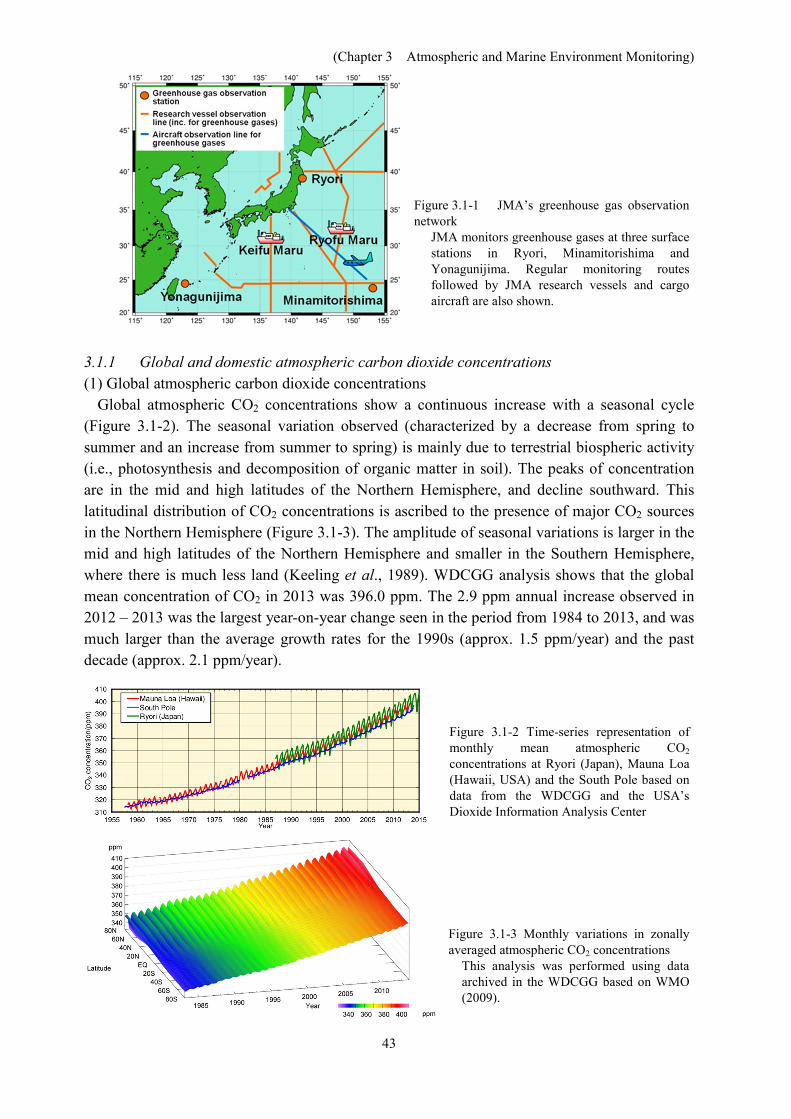
Figure 3.1-1 JMA’s greenhouse gas observation network

JMA monitors greenhouse gases at three surface stations in Ryori, Minamitorishima and Yonagunijima. Regular monitoring routes followed by JMA research vessels and cargo aircraft are also shown.

3.1.1 Global and domestic atmospheric carbon dioxide concentrations (1) Global atmospheric carbon dioxide concentrations

Global atmospheric CO2 concentrations show a continuous increase with a seasonal cycle (Figure 3.1-2). The seasonal variation observed (characterized by a decrease from spring to summer and an increase from summer to spring) is mainly due to terrestrial biospheric activity (i.e., photosynthesis and decomposition of organic matter in soil). The peaks of concentration are in the mid and high latitudes of the Northern Hemisphere, and decline southward. This latitudinal distribution of CO2 concentrations is ascribed to the presence of major CO2 sources in the Northern Hemisphere (Figure 3.1-3). The amplitude of seasonal variations is larger in the mid and high latitudes of the Northern Hemisphere and smaller in the Southern Hemisphere, where there is much less land (Keeling et al., 1989). WDCGG analysis shows that the global mean concentration of CO2 in 2013 was 396.0 ppm. The 2.9 ppm annual increase observed in 2012 – 2013 was the largest year-on-year change seen in the period from 1984 to 2013, and was much larger than the average growth rates for the 1990s (approx. 1.5 ppm/year) and the past decade (approx. 2.1 ppm/year).

Figure 3.1-2 Time-series representation of monthly mean atmospheric CO2 concentrations at Ryori (Japan), Mauna Loa (Hawaii, USA) and the South Pole based on data from the WDCGG and the USA’s Dioxide Information Analysis Center

Figure 3.1-3 Monthly variations in zonally averaged atmospheric CO2 concentrations

This analysis was performed using data archived in the WDCGG based on WMO (2009).

(Chapter 3 Atmospheric and Marine Environment Monitoring)

44

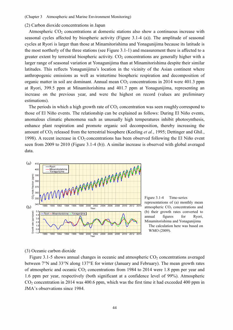
(2) Carbon dioxide concentrations in Japan Atmospheric CO2 concentrations at domestic stations also show a continuous increase with

seasonal cycles affected by biospheric activity (Figure 3.1-4 (a)). The amplitude of seasonal cycles at Ryori is larger than those at Minamitorishima and Yonagunijima because its latitude is the most northerly of the three stations (see Figure 3.1-1) and measurement there is affected to a greater extent by terrestrial biospheric activity. CO2 concentrations are generally higher with a larger range of seasonal variation at Yonagunijima than at Minamitorishima despite their similar latitudes. This reflects Yonagunijima’s location in the vicinity of the Asian continent where anthropogenic emissions as well as wintertime biospheric respiration and decomposition of organic matter in soil are dominant. Annual mean CO2 concentrations in 2014 were 401.3 ppm at Ryori, 399.5 ppm at Minamitorishima and 401.7 ppm at Yonagunijima, representing an increase on the previous year, and were the highest on record (values are preliminary estimations).

The periods in which a high growth rate of CO2 concentration was seen roughly correspond to those of El Niño events. The relationship can be explained as follows: During El Niño events, anomalous climatic phenomena such as unusually high temperatures inhibit photosynthesis, enhance plant respiration and promote organic soil decomposition, thereby increasing the amount of CO2 released from the terrestrial biosphere (Keeling et al., 1995; Dettinger and Ghil., 1998). A recent increase in CO2 concentrations has been observed following the El Niño event seen from 2009 to 2010 (Figure 3.1-4 (b)). A similar increase is observed with global averaged data.

(a) (b)

Figure 3.1-4 Time-series representations of (a) monthly mean atmospheric CO2 concentrations and (b) their growth rates converted to annual figures for Ryori, Minamitorishima and Yonagunijima

The calculation here was based on WMO (2009).

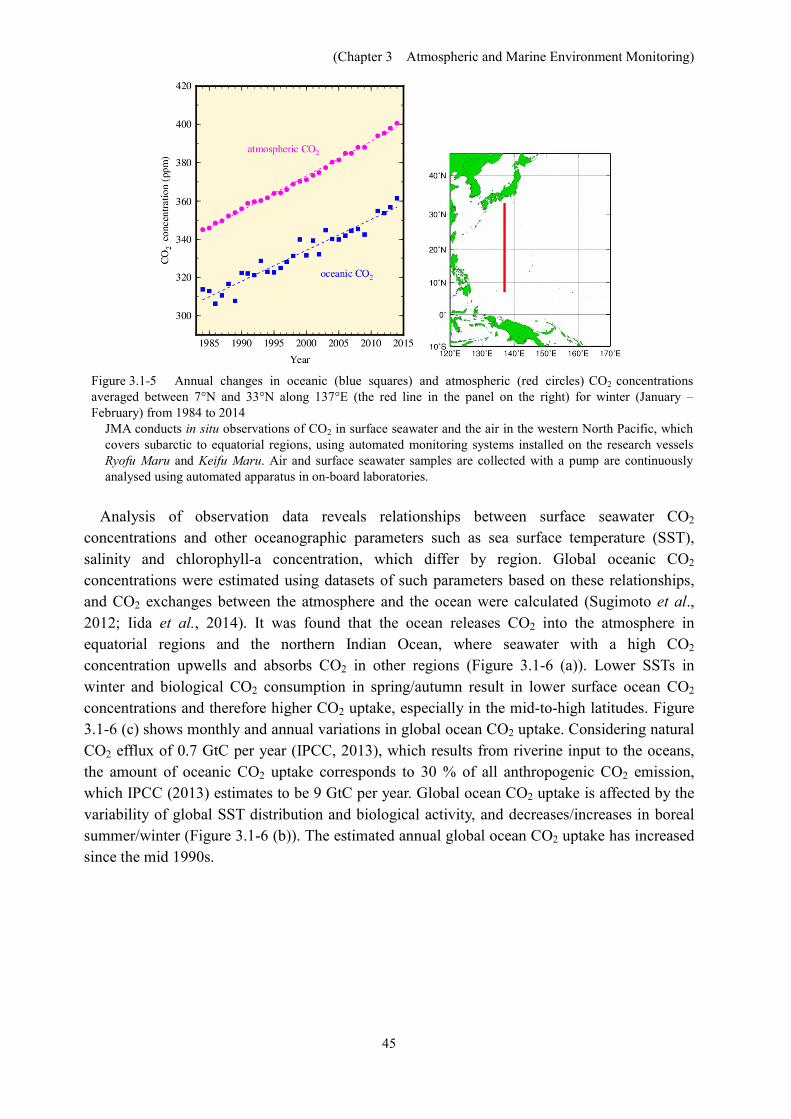
(3) Oceanic carbon dioxide Figure 3.1-5 shows annual changes in oceanic and atmospheric CO2 concentrations averaged

between 7°N and 33°N along 137°E for winter (January and February). The mean growth rates of atmospheric and oceanic CO2 concentrations from 1984 to 2014 were 1.8 ppm per year and 1.6 ppm per year, respectively (both significant at a confidence level of 99%). Atmospheric CO2 concentration in 2014 was 400.6 ppm, which was the first time it had exceeded 400 ppm in JMA’s observations since 1984.

(Chapter 3 Atmospheric and Marine Environment Monitoring)

45

Figure 3.1-5 Annual changes in oceanic (blue squares) and atmospheric (red circles) CO2 concentrations averaged between 7°N and 33°N along 137°E (the red line in the panel on the right) for winter (January – February) from 1984 to 2014

JMA conducts in situ observations of CO2 in surface seawater and the air in the western North Pacific, which covers subarctic to equatorial regions, using automated monitoring systems installed on the research vessels Ryofu Maru and Keifu Maru. Air and surface seawater samples are collected with a pump are continuously analysed using automated apparatus in on-board laboratories.

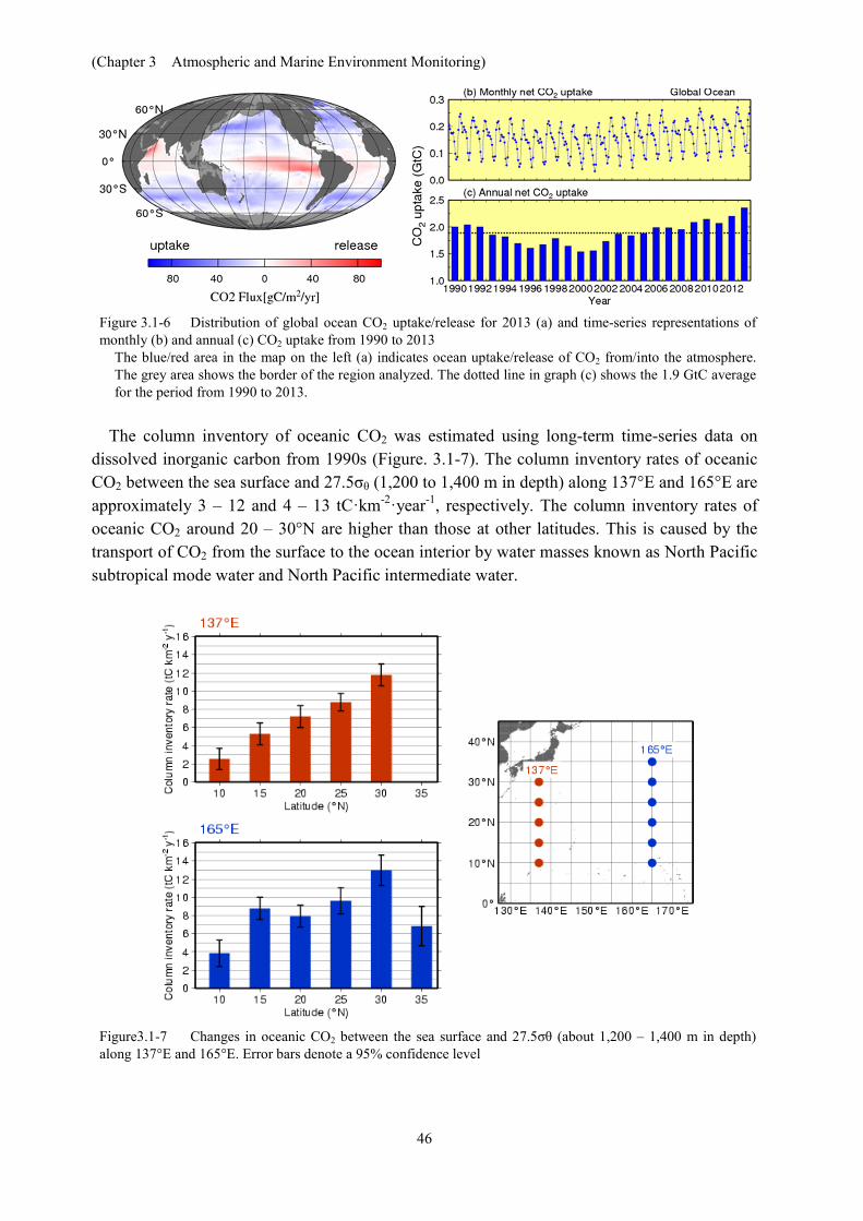
Analysis of observation data reveals relationships between surface seawater CO2 concentrations and other oceanographic parameters such as sea surface temperature (SST), salinity and chlorophyll-a concentration, which differ by region. Global oceanic CO2 concentrations were estimated using datasets of such parameters based on these relationships, and CO2 exchanges between the atmosphere and the ocean were calculated (Sugimoto et al., 2012; Iida et al., 2014). It was found that the ocean releases CO2 into the atmosphere in equatorial regions and the northern Indian Ocean, where seawater with a high CO2 concentration upwells and absorbs CO2 in other regions (Figure 3.1-6 (a)). Lower SSTs in winter and biological CO2 consumption in spring/autumn result in lower surface ocean CO2 concentrations and therefore higher CO2 uptake, especially in the mid-to-high latitudes. Figure 3.1-6 (c) shows monthly and annual variations in global ocean CO2 uptake. Considering natural CO2 efflux of 0.7 GtC per year (IPCC, 2013), which results from riverine input to the oceans, the amount of oceanic CO2 uptake corresponds to 30 % of all anthropogenic CO2 emission, which IPCC (2013) estimates to be 9 GtC per year. Global ocean CO2 uptake is affected by the variability of global SST distribution and biological activity, and decreases/increases in boreal summer/winter (Figure 3.1-6 (b)). The estimated annual global ocean CO2 uptake has increased since the mid 1990s.

(Chapter 3 Atmospheric and Marine Environment Monitoring)

46

Figure 3.1-6 Distribution of global ocean CO2 uptake/release for 2013 (a) and time-series representations of monthly (b) and annual (c) CO2 uptake from 1990 to 2013

The blue/red area in the map on the left (a) indicates ocean uptake/release of CO2 from/into the atmosphere. The grey area shows the border of the region analyzed. The dotted line in graph (c) shows the 1.9 GtC average for the period from 1990 to 2013.

The column inventory of oceanic CO2 was estimated using long-term time-series data on

dissolved inorganic carbon from 1990s (Figure. 3.1-7). The column inventory rates of oceanic CO2 between the sea surface and 27.5σθ (1,200 to 1,400 m in depth) along 137°E and 165°E are approximately 3 – 12 and 4 – 13 tC·km-2·year-1, respectively. The column inventory rates of oceanic CO2 around 20 – 30°N are higher than those at other latitudes. This is caused by the transport of CO2 from the surface to the ocean interior by water masses known as North Pacific subtropical mode water and North Pacific intermediate water.

Figure3.1-7 Changes in oceanic CO2 between the sea surface and 27.5σθ (about 1,200 – 1,400 m in depth) along 137°E and 165°E. Error bars denote a 95% confidence level

(Chapter 3 Atmospheric and Marine Environment Monitoring)

47

(4) Ocean acidification The oceans are the earth’s largest sinks for CO2 emitted as a result of human activities, and

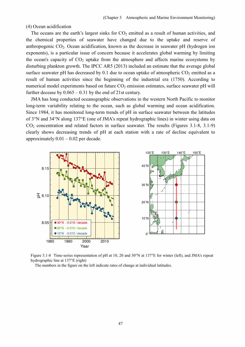
the chemical properties of seawater have changed due to the uptake and reserve of anthropogenic CO2. Ocean acidification, known as the decrease in seawater pH (hydrogen ion exponents), is a particular issue of concern because it accelerates global warming by limiting the ocean's capacity of CO2 uptake from the atmosphere and affects marine ecosystems by disturbing plankton growth. The IPCC AR5 (2013) included an estimate that the average global surface seawater pH has decreased by 0.1 due to ocean uptake of atmospheric CO2 emitted as a result of human activities since the beginning of the industrial era (1750). According to numerical model experiments based on future CO2 emission estimates, surface seawater pH will further decease by 0.065 – 0.31 by the end of 21st century.

JMA has long conducted oceanographic observations in the western North Pacific to monitor long-term variability relating to the ocean, such as global warming and ocean acidification. Since 1984, it has monitored long-term trends of pH in surface seawater between the latitudes of 3°N and 34°N along 137°E (one of JMA’s repeat hydrographic lines) in winter using data on CO2 concentration and related factors in surface seawater. The results (Figures 3.1-8, 3.1-9) clearly shows decreasing trends of pH at each station with a rate of decline equivalent to approximately 0.01 – 0.02 per decade.

Figure 3.1-8 Time-series representation of pH at 10, 20 and 30°N at 137°E for winter (left), and JMA’s repeat hydrographic line at 137°E (right)

The numbers in the figure on the left indicate rates of change at individual latitudes.

(Chapter 3 Atmospheric and Marine Environment Monitoring)

48

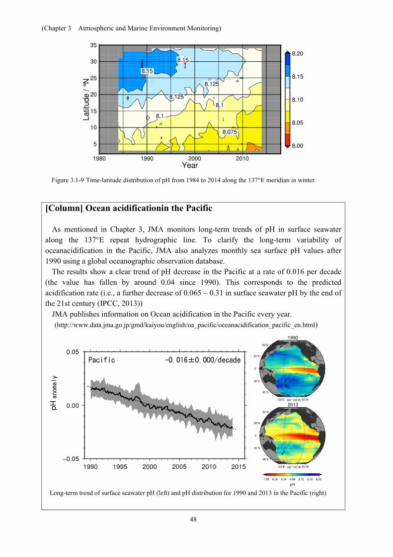
Figure 3.1-9 Time-latitude distribution of pH from 1984 to 2014 along the 137°E meridian in winter.

[Column] Ocean acidificationin the Pacific As mentioned in Chapter 3, JMA monitors long-term trends of pH in surface seawater

along the 137°E repeat hydrographic line. To clarify the long-term variability of oceanacidification in the Pacific, JMA also analyzes monthly sea surface pH values after 1990 using a global oceanographic observation database.

The results show a clear trend of pH decrease in the Pacific at a rate of 0.016 per decade (the value has fallen by around 0.04 since 1990). This corresponds to the predicted acidification rate (i.e., a further decrease of 0.065 – 0.31 in surface seawater pH by the end of the 21st century (IPCC, 2013))

JMA publishes information on Ocean acidification in the Pacific every year. (http://www.data.jma.go.jp/gmd/kaiyou/english/oa_pacific/oceanacidification_pacific_en.html)

Long-term trend of surface seawater pH (left) and pH distribution for 1990 and 2013 in the Pacific (right)

(Chapter 3 Atmospheric and Marine Environment Monitoring)

49

(5) Upper-troposphere monitoring of carbon dioxide The National Institute for Environment Studies and the Meteorological Research Institute

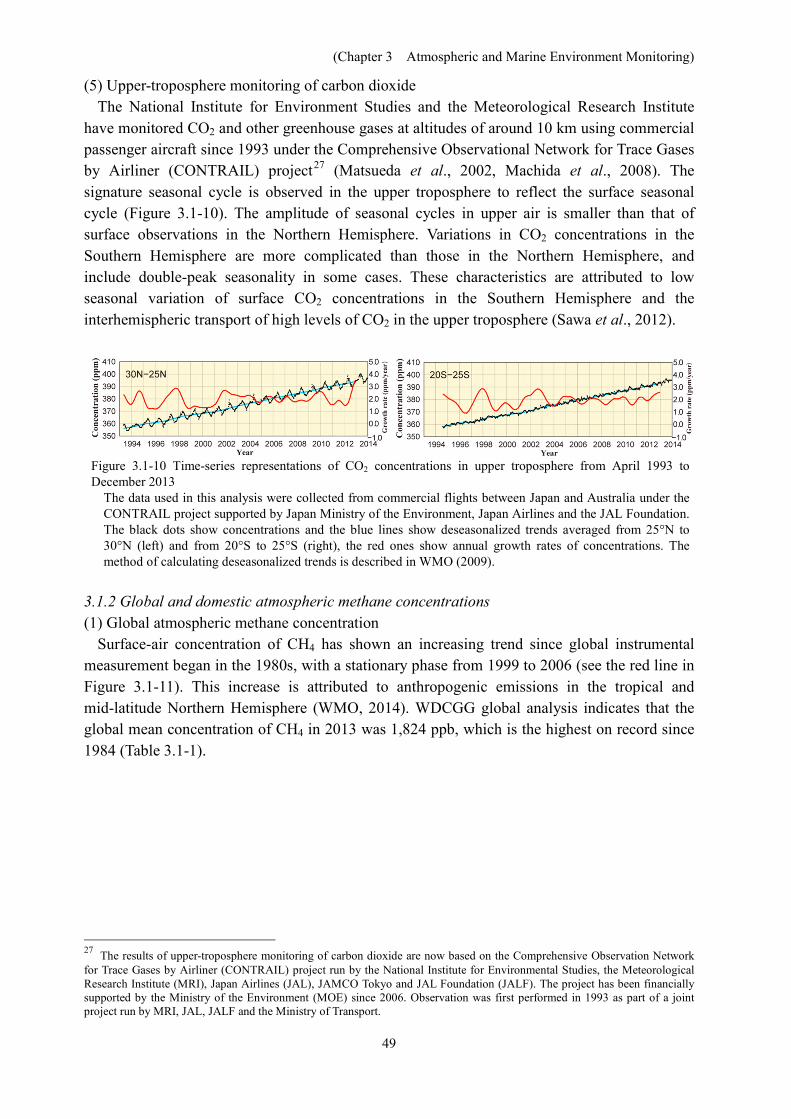
have monitored CO2 and other greenhouse gases at altitudes of around 10 km using commercial passenger aircraft since 1993 under the Comprehensive Observational Network for Trace Gases by Airliner (CONTRAIL) project27 (Matsueda et al., 2002, Machida et al., 2008). The signature seasonal cycle is observed in the upper troposphere to reflect the surface seasonal cycle (Figure 3.1-10). The amplitude of seasonal cycles in upper air is smaller than that of surface observations in the Northern Hemisphere. Variations in CO2 concentrations in the Southern Hemisphere are more complicated than those in the Northern Hemisphere, and include double-peak seasonality in some cases. These characteristics are attributed to low seasonal variation of surface CO2 concentrations in the Southern Hemisphere and the interhemispheric transport of high levels of CO2 in the upper troposphere (Sawa et al., 2012).

Figure 3.1-10 Time-series representations of CO2 concentrations in upper troposphere from April 1993 to December 2013

The data used in this analysis were collected from commercial flights between Japan and Australia under the CONTRAIL project supported by Japan Ministry of the Environment, Japan Airlines and the JAL Foundation. The black dots show concentrations and the blue lines show deseasonalized trends averaged from 25°N to 30°N (left) and from 20°S to 25°S (right), the red ones show annual growth rates of concentrations. The method of calculating deseasonalized trends is described in WMO (2009).

3.1.2 Global and domestic atmospheric methane concentrations (1) Global atmospheric methane concentration

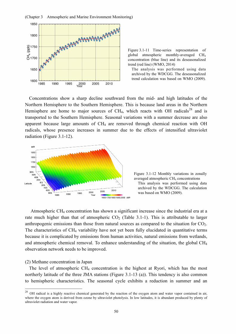
Surface-air concentration of CH4 has shown an increasing trend since global instrumental measurement began in the 1980s, with a stationary phase from 1999 to 2006 (see the red line in Figure 3.1-11). This increase is attributed to anthropogenic emissions in the tropical and mid-latitude Northern Hemisphere (WMO, 2014). WDCGG global analysis indicates that the global mean concentration of CH4 in 2013 was 1,824 ppb, which is the highest on record since 1984 (Table 3.1-1).

27 The results of upper-troposphere monitoring of carbon dioxide are now based on the Comprehensive Observation Network for Trace Gases by Airliner (CONTRAIL) project run by the National Institute for Environmental Studies, the Meteorological Research Institute (MRI), Japan Airlines (JAL), JAMCO Tokyo and JAL Foundation (JALF). The project has been financially supported by the Ministry of the Environment (MOE) since 2006. Observation was first performed in 1993 as part of a joint project run by MRI, JAL, JALF and the Ministry of Transport.

(Chapter 3 Atmospheric and Marine Environment Monitoring)

50

Figure 3.1-11 Time-series representation of global atmospheric monthly-averaged CH4 concentration (blue line) and its deseasonalized trend (red line) (WMO, 2014)

The analysis was performed using data archived by the WDCGG. The deseasonalized trend calculation was based on WMO (2009).

Concentrations show a sharp decline southward from the mid- and high latitudes of the Northern Hemisphere to the Southern Hemisphere. This is because land areas in the Northern Hemisphere are home to major sources of CH4, which reacts with OH radicals28 and is transported to the Southern Hemisphere. Seasonal variations with a summer decrease are also apparent because large amounts of CH4 are removed through chemical reaction with OH radicals, whose presence increases in summer due to the effects of intensified ultraviolet radiation (Figure 3.1-12).

Figure 3.1-12 Monthly variations in zonally averaged atmospheric CH4 concentrations

This analysis was performed using data archived by the WDCGG. The calculation was based on WMO (2009).

Atmospheric CH4 concentration has shown a significant increase since the industrial era at a rate much higher than that of atmospheric CO2 (Table 3.1-1). This is attributable to larger anthropogenic emissions than those from natural sources as compared to the situation for CO2. The characteristics of CH4 variability have not yet been fully elucidated in quantitative terms because it is complicated by emissions from human activities, natural emissions from wetlands, and atmospheric chemical removal. To enhance understanding of the situation, the global CH4 observation network needs to be improved. (2) Methane concentration in Japan

The level of atmospheric CH4 concentration is the highest at Ryori, which has the most northerly latitude of the three JMA stations (Figure 3.1-13 (a)). This tendency is also common to hemispheric characteristics. The seasonal cycle exhibits a reduction in summer and an 28 OH radical is a highly reactive chemical generated by the reaction of the oxygen atom and water vapor contained in air, where the oxygen atom is derived from ozone by ultraviolet photolysis. In low latitudes, it is abundant produced by plenty of ultraviolet radiation and water vapor.

(Chapter 3 Atmospheric and Marine Environment Monitoring)

51

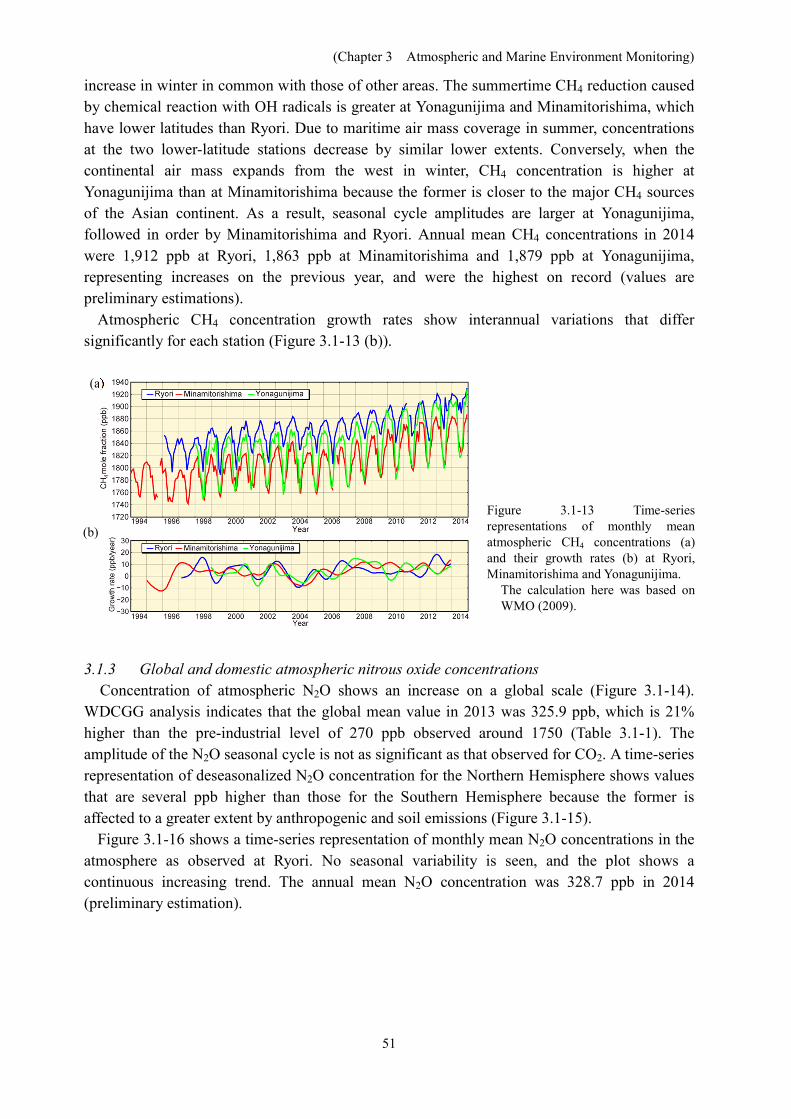
increase in winter in common with those of other areas. The summertime CH4 reduction caused by chemical reaction with OH radicals is greater at Yonagunijima and Minamitorishima, which have lower latitudes than Ryori. Due to maritime air mass coverage in summer, concentrations at the two lower-latitude stations decrease by similar lower extents. Conversely, when the continental air mass expands from the west in winter, CH4 concentration is higher at Yonagunijima than at Minamitorishima because the former is closer to the major CH4 sources of the Asian continent. As a result, seasonal cycle amplitudes are larger at Yonagunijima, followed in order by Minamitorishima and Ryori. Annual mean CH4 concentrations in 2014 were 1,912 ppb at Ryori, 1,863 ppb at Minamitorishima and 1,879 ppb at Yonagunijima, representing increases on the previous year, and were the highest on record (values are preliminary estimations).

Atmospheric CH4 concentration growth rates show interannual variations that differ significantly for each station (Figure 3.1-13 (b)). (a)

(b)

Figure 3.1-13 Time-series representations of monthly mean atmospheric CH4 concentrations (a) and their growth rates (b) at Ryori, Minamitorishima and Yonagunijima.

The calculation here was based on WMO (2009).

3.1.3 Global and domestic atmospheric nitrous oxide concentrations

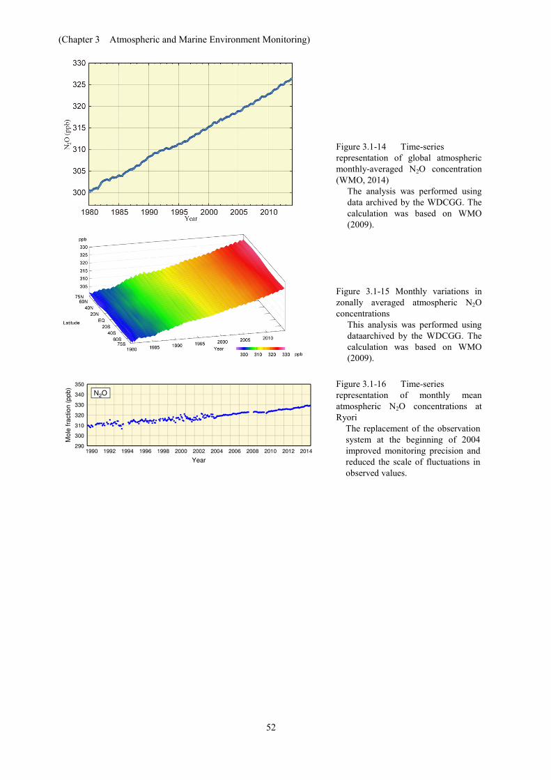
Concentration of atmospheric N2O shows an increase on a global scale (Figure 3.1-14). WDCGG analysis indicates that the global mean value in 2013 was 325.9 ppb, which is 21% higher than the pre-industrial level of 270 ppb observed around 1750 (Table 3.1-1). The amplitude of the N2O seasonal cycle is not as significant as that observed for CO2. A time-series representation of deseasonalized N2O concentration for the Northern Hemisphere shows values that are several ppb higher than those for the Southern Hemisphere because the former is affected to a greater extent by anthropogenic and soil emissions (Figure 3.1-15).

Figure 3.1-16 shows a time-series representation of monthly mean N2O concentrations in the atmosphere as observed at Ryori. No seasonal variability is seen, and the plot shows a continuous increasing trend. The annual mean N2O concentration was 328.7 ppb in 2014 (preliminary estimation).

(Chapter 3 Atmospheric and Marine Environment Monitoring)

52

Figure 3.1-14 Time-series representation of global atmospheric monthly-averaged N2O concentration (WMO, 2014)

The analysis was performed using data archived by the WDCGG. The calculation was based on WMO (2009).

Figure 3.1-15 Monthly variations in zonally averaged atmospheric N2O concentrations

This analysis was performed using dataarchived by the WDCGG. The calculation was based on WMO (2009).

Figure 3.1-16 Time-series representation of monthly mean atmospheric N2O concentrations at Ryori

The replacement of the observation system at the beginning of 2004 improved monitoring precision and reduced the scale of fluctuations in observed values.

(Chapter 3 Atmospheric and Marine Environment Monitoring)

53

3.2 Monitoring of the ozone layer and ultraviolet radiation29

○ Global atmospheric concentrations of chlorofluorocarbons (CFCs) have gradually decreased in recent years.

○ Global-averaged total ozone amount decreased significantly in the 1980s and the early 1990s, and remains low today with a slightly increasing trend.

○ The annual maximum area of the ozone hole in the Southern Hemisphere increased substantially in the 1980s and 1990s, but no discernible trend was observed in the 2000s.

○ Increasing trends in annual cumulative daily erythemal UV radiation have been observed at Sapporo and Tsukuba since the early 1990s.

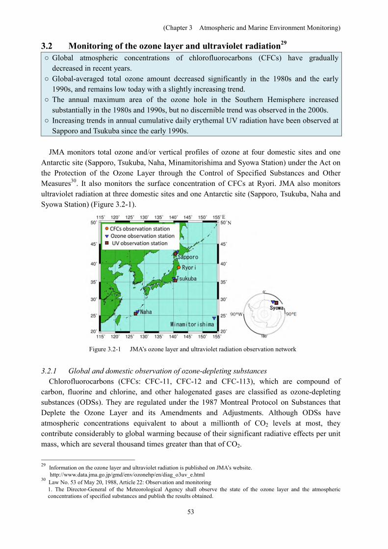
JMA monitors total ozone and/or vertical profiles of ozone at four domestic sites and one

Antarctic site (Sapporo, Tsukuba, Naha, Minamitorishima and Syowa Station) under the Act on the Protection of the Ozone Layer through the Control of Specified Substances and Other Measures30. It also monitors the surface concentration of CFCs at Ryori. JMA also monitors ultraviolet radiation at three domestic sites and one Antarctic site (Sapporo, Tsukuba, Naha and Syowa Station) (Figure 3.2-1).

Figure 3.2-1 JMA’s ozone layer and ultraviolet radiation observation network

3.2.1 Global and domestic observation of ozone-depleting substances

Chlorofluorocarbons (CFCs: CFC-11, CFC-12 and CFC-113), which are compound of carbon, fluorine and chlorine, and other halogenated gases are classified as ozone-depleting substances (ODSs). They are regulated under the 1987 Montreal Protocol on Substances that Deplete the Ozone Layer and its Amendments and Adjustments. Although ODSs have atmospheric concentrations equivalent to about a millionth of CO2 levels at most, they contribute considerably to global warming because of their significant radiative effects per unit mass, which are several thousand times greater than that of CO2.

29 Information on the ozone layer and ultraviolet radiation is published on JMA’s website.

http://www.data.jma.go.jp/gmd/env/ozonehp/en/diag_o3uv_e.html 30 Law No. 53 of May 20, 1988, Article 22: Observation and monitoring

1. The Director-General of the Meteorological Agency shall observe the state of the ozone layer and the atmospheric concentrations of specified substances and publish the results obtained.

E N

(Chapter 3 Atmospheric and Marine Environment Monitoring)

54

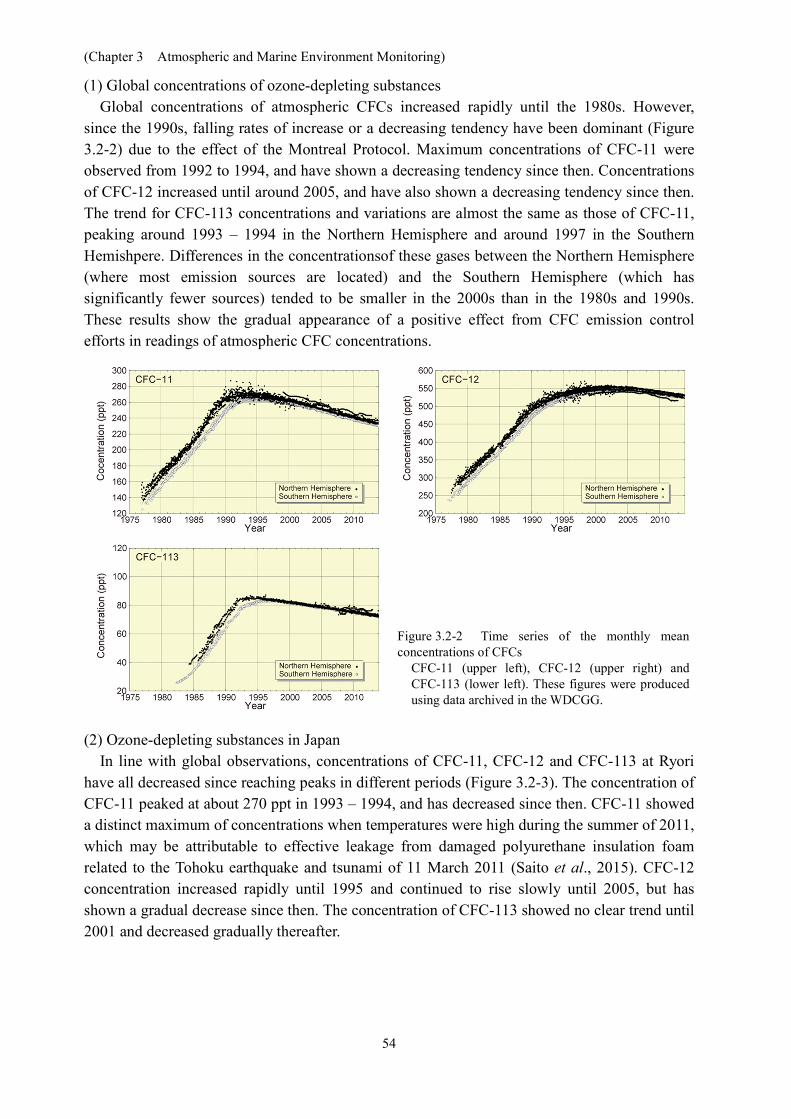
(1) Global concentrations of ozone-depleting substances Global concentrations of atmospheric CFCs increased rapidly until the 1980s. However,

since the 1990s, falling rates of increase or a decreasing tendency have been dominant (Figure 3.2-2) due to the effect of the Montreal Protocol. Maximum concentrations of CFC-11 were observed from 1992 to 1994, and have shown a decreasing tendency since then. Concentrations of CFC-12 increased until around 2005, and have also shown a decreasing tendency since then. The trend for CFC-113 concentrations and variations are almost the same as those of CFC-11, peaking around 1993 – 1994 in the Northern Hemisphere and around 1997 in the Southern Hemishpere. Differences in the concentrationsof these gases between the Northern Hemisphere (where most emission sources are located) and the Southern Hemisphere (which has significantly fewer sources) tended to be smaller in the 2000s than in the 1980s and 1990s. These results show the gradual appearance of a positive effect from CFC emission control efforts in readings of atmospheric CFC concentrations.

Figure 3.2-2 Time series of the monthly mean concentrations of CFCs

CFC-11 (upper left), CFC-12 (upper right) and CFC-113 (lower left). These figures were produced using data archived in the WDCGG.

(2) Ozone-depleting substances in Japan

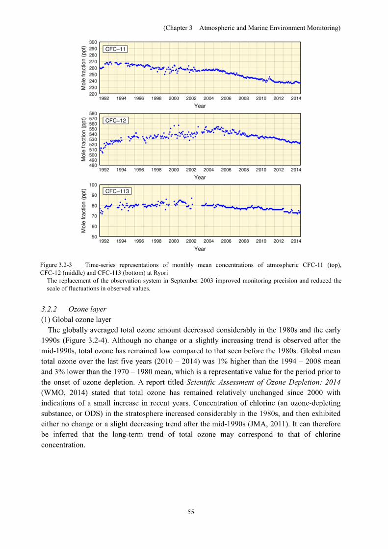
In line with global observations, concentrations of CFC-11, CFC-12 and CFC-113 at Ryori have all decreased since reaching peaks in different periods (Figure 3.2-3). The concentration of CFC-11 peaked at about 270 ppt in 1993 – 1994, and has decreased since then. CFC-11 showed a distinct maximum of concentrations when temperatures were high during the summer of 2011, which may be attributable to effective leakage from damaged polyurethane insulation foam related to the Tohoku earthquake and tsunami of 11 March 2011 (Saito et al., 2015). CFC-12 concentration increased rapidly until 1995 and continued to rise slowly until 2005, but has shown a gradual decrease since then. The concentration of CFC-113 showed no clear trend until 2001 and decreased gradually thereafter.

(Chapter 3 Atmospheric and Marine Environment Monitoring)

55

Figure 3.2-3 Time-series representations of monthly mean concentrations of atmospheric CFC-11 (top), CFC-12 (middle) and CFC-113 (bottom) at Ryori

The replacement of the observation system in September 2003 improved monitoring precision and reduced the scale of fluctuations in observed values.

3.2.2 Ozone layer (1) Global ozone layer

The globally averaged total ozone amount decreased considerably in the 1980s and the early 1990s (Figure 3.2-4). Although no change or a slightly increasing trend is observed after the mid-1990s, total ozone has remained low compared to that seen before the 1980s. Global mean total ozone over the last five years (2010 – 2014) was 1% higher than the 1994 – 2008 mean and 3% lower than the 1970 – 1980 mean, which is a representative value for the period prior to the onset of ozone depletion. A report titled Scientific Assessment of Ozone Depletion: 2014 (WMO, 2014) stated that total ozone has remained relatively unchanged since 2000 with indications of a small increase in recent years. Concentration of chlorine (an ozone-depleting substance, or ODS) in the stratosphere increased considerably in the 1980s, and then exhibited either no change or a slight decreasing trend after the mid-1990s (JMA, 2011). It can therefore be inferred that the long-term trend of total ozone may correspond to that of chlorine concentration.

(Chapter 3 Atmospheric and Marine Environment Monitoring)

56

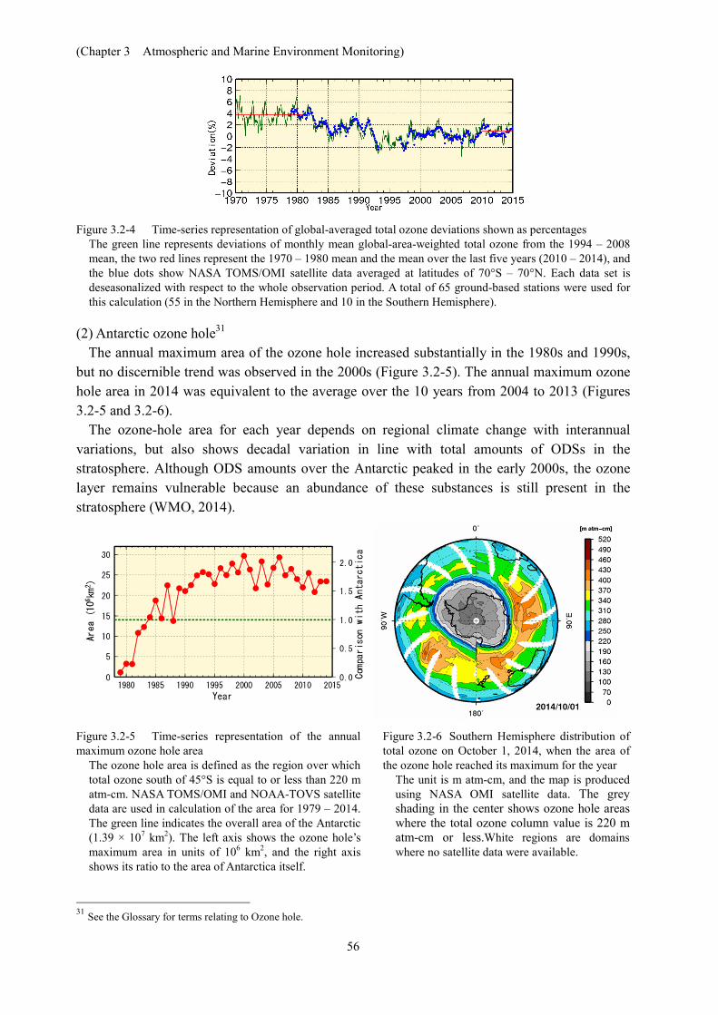
Figure 3.2-4 Time-series representation of global-averaged total ozone deviations shown as percentages

The green line represents deviations of monthly mean global-area-weighted total ozone from the 1994 – 2008 mean, the two red lines represent the 1970 – 1980 mean and the mean over the last five years (2010 – 2014), and the blue dots show NASA TOMS/OMI satellite data averaged at latitudes of 70°S – 70°N. Each data set is deseasonalized with respect to the whole observation period. A total of 65 ground-based stations were used for this calculation (55 in the Northern Hemisphere and 10 in the Southern Hemisphere).

(2) Antarctic ozone hole31

The annual maximum area of the ozone hole increased substantially in the 1980s and 1990s, but no discernible trend was observed in the 2000s (Figure 3.2-5). The annual maximum ozone hole area in 2014 was equivalent to the average over the 10 years from 2004 to 2013 (Figures 3.2-5 and 3.2-6).

The ozone-hole area for each year depends on regional climate change with interannual variations, but also shows decadal variation in line with total amounts of ODSs in the stratosphere. Although ODS amounts over the Antarctic peaked in the early 2000s, the ozone layer remains vulnerable because an abundance of these substances is still present in the stratosphere (WMO, 2014).

Figure 3.2-5 Time-series representation of the annual maximum ozone hole area

The ozone hole area is defined as the region over which total ozone south of 45°S is equal to or less than 220 m atm-cm. NASA TOMS/OMI and NOAA-TOVS satellite data are used in calculation of the area for 1979 – 2014. The green line indicates the overall area of the Antarctic (1.39 × 107 km2). The left axis shows the ozone hole’s maximum area in units of 106 km2, and the right axis shows its ratio to the area of Antarctica itself.

Figure 3.2-6 Southern Hemisphere distribution of total ozone on October 1, 2014, when the area of the ozone hole reached its maximum for the year

The unit is m atm-cm, and the map is produced using NASA OMI satellite data. The grey shading in the center shows ozone hole areas where the total ozone column value is 220 m atm-cm or less.White regions are domains where no satellite data were available.

31 See the Glossary for terms relating to Ozone hole.

(Chapter 3 Atmospheric and Marine Environment Monitoring)

57

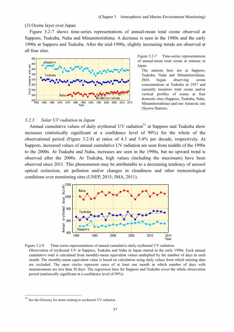
(3) Ozone layer over Japan Figure 3.2-7 shows time-series representations of annual-mean total ozone observed at

Sapporo, Tsukuba, Naha and Minamitorishima. A decrease is seen in the 1980s and the early 1990s at Sapporo and Tsukuba. After the mid-1990s, slightly increasing trends are observed at all four sites.

Figure 3.2-7 Time-series representations of annual-mean total ozone at stations in Japan

The stations here are at Sapporo, Tsukuba, Naha and Minamitorishima. JMA began observing ozone concentrations at Tsukuba in 1957 and currently monitors total ozone and/or vertical profiles of ozone at four domestic sites (Sapporo, Tsukuba, Naha, Minamitorishima) and one Antarctic site (Syowa Station).

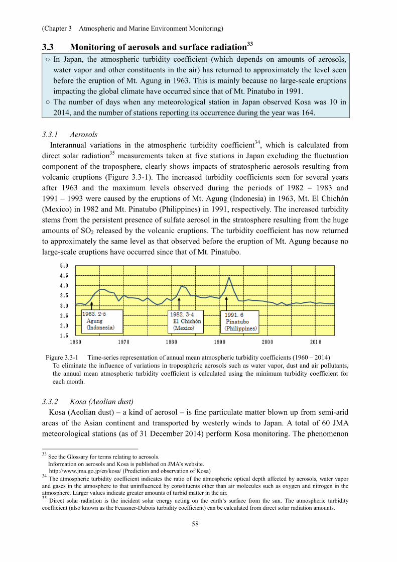
3.2.3 Solar UV radiation in Japan Annual cumulative values of daily erythemal UV radiation32 at Sapporo and Tsukuba show

increases (statistically significant at a confidence level of 99%) for the whole of the observational period (Figure 3.2-8) at ratios of 4.3 and 5.4% per decade, respectively. At Sapporo, increased values of annual cumulative UV radiation are seen from middle of the 1990s to the 2000s. At Tsukuba and Naha, increases are seen in the 1990s, but no upward trend is observed after the 2000s. At Tsukuba, high values (including the maximum) have been observed since 2011. This phenomenon may be attributable to a decreasing tendency of aerosol optical extinction, air pollution and/or changes in cloudiness and other meteorological conditions over monitoring sites (UNEP, 2015; JMA, 2011).

Figure 3.2-8 Time-series representations of annual cumulative daily erythemal UV radiation Observation of erythemal UV at Sapporo, Tsukuba and Naha in Japan started in the early 1990s. Each annual cumulative total is calculated from monthly-mean equivalent values multiplied by the number of days in each month. The monthly-mean equivalent value is based on calculation using daily values from which missing data are excluded. The open circles represent cases of at least one month in which number of days with measurements are less than 20 days. The regression lines for Sapporo and Tsukuba cover the whole observation period (statistically significant at a confidence level of 99%).

32 See the Glossary for terms relating to erythemal UV radiation.

(Chapter 3 Atmospheric and Marine Environment Monitoring)

58

3.3 Monitoring of aerosols and surface radiation33 ○ In Japan, the atmospheric turbidity coefficient (which depends on amounts of aerosols,

water vapor and other constituents in the air) has returned to approximately the level seen before the eruption of Mt. Agung in 1963. This is mainly because no large-scale eruptions impacting the global climate have occurred since that of Mt. Pinatubo in 1991.

○ The number of days when any meteorological station in Japan observed Kosa was 10 in 2014, and the number of stations reporting its occurrence during the year was 164.

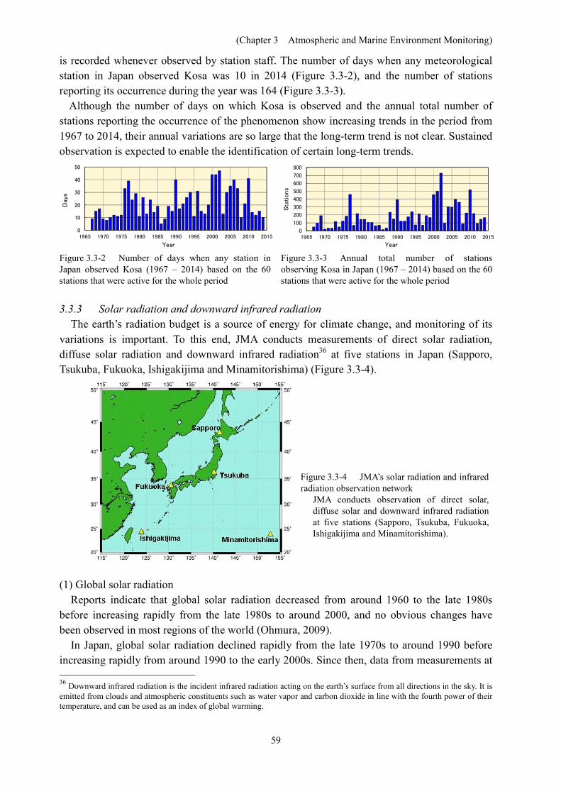
3.3.1 Aerosols Interannual variations in the atmospheric turbidity coefficient34, which is calculated from

direct solar radiation35 measurements taken at five stations in Japan excluding the fluctuation component of the troposphere, clearly shows impacts of stratospheric aerosols resulting from volcanic eruptions (Figure 3.3-1). The increased turbidity coefficients seen for several years after 1963 and the maximum levels observed during the periods of 1982 – 1983 and 1991 – 1993 were caused by the eruptions of Mt. Agung (Indonesia) in 1963, Mt. El Chichón (Mexico) in 1982 and Mt. Pinatubo (Philippines) in 1991, respectively. The increased turbidity stems from the persistent presence of sulfate aerosol in the stratosphere resulting from the huge amounts of SO2 released by the volcanic eruptions. The turbidity coefficient has now returned to approximately the same level as that observed before the eruption of Mt. Agung because no large-scale eruptions have occurred since that of Mt. Pinatubo.

Figure 3.3-1 Time-series representation of annual mean atmospheric turbidity coefficients (1960 – 2014)

To eliminate the influence of variations in tropospheric aerosols such as water vapor, dust and air pollutants, the annual mean atmospheric turbidity coefficient is calculated using the minimum turbidity coefficient for each month.

3.3.2 Kosa (Aeolian dust)

Kosa (Aeolian dust) – a kind of aerosol – is fine particulate matter blown up from semi-arid areas of the Asian continent and transported by westerly winds to Japan. A total of 60 JMA meteorological stations (as of 31 December 2014) perform Kosa monitoring. The phenomenon

33 See the Glossary for terms relating to aerosols. Information on aerosols and Kosa is published on JMA’s website.

http://www.jma.go.jp/en/kosa/ (Prediction and observation of Kosa) 34 The atmospheric turbidity coefficient indicates the ratio of the atmospheric optical depth affected by aerosols, water vapor and gases in the atmosphere to that uninfluenced by constituents other than air molecules such as oxygen and nitrogen in the atmosphere. Larger values indicate greater amounts of turbid matter in the air. 35 Direct solar radiation is the incident solar energy acting on the earth’s surface from the sun. The atmospheric turbidity coefficient (also known as the Feussner-Dubois turbidity coefficient) can be calculated from direct solar radiation amounts.

(Chapter 3 Atmospheric and Marine Environment Monitoring)

59

is recorded whenever observed by station staff. The number of days when any meteorological station in Japan observed Kosa was 10 in 2014 (Figure 3.3-2), and the number of stations reporting its occurrence during the year was 164 (Figure 3.3-3).

Although the number of days on which Kosa is observed and the annual total number of stations reporting the occurrence of the phenomenon show increasing trends in the period from 1967 to 2014, their annual variations are so large that the long-term trend is not clear. Sustained observation is expected to enable the identification of certain long-term trends.

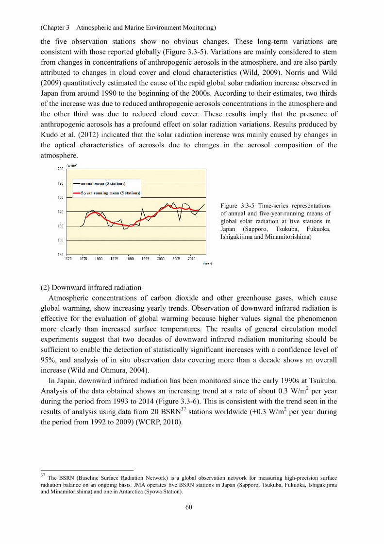
3.3.3 Solar radiation and downward infrared radiation The earth’s radiation budget is a source of energy for climate change, and monitoring of its

variations is important. To this end, JMA conducts measurements of direct solar radiation, diffuse solar radiation and downward infrared radiation36 at five stations in Japan (Sapporo, Tsukuba, Fukuoka, Ishigakijima and Minamitorishima) (Figure 3.3-4).

Figure 3.3-4 JMA’s solar radiation and infrared radiation observation network

JMA conducts observation of direct solar, diffuse solar and downward infrared radiation at five stations (Sapporo, Tsukuba, Fukuoka, Ishigakijima and Minamitorishima).

(1) Global solar radiation

Reports indicate that global solar radiation decreased from around 1960 to the late 1980s before increasing rapidly from the late 1980s to around 2000, and no obvious changes have been observed in most regions of the world (Ohmura, 2009).

In Japan, global solar radiation declined rapidly from the late 1970s to around 1990 before increasing rapidly from around 1990 to the early 2000s. Since then, data from measurements at 36 Downward infrared radiation is the incident infrared radiation acting on the earth’s surface from all directions in the sky. It is emitted from clouds and atmospheric constituents such as water vapor and carbon dioxide in line with the fourth power of their temperature, and can be used as an index of global warming.

Figure 3.3-2 Number of days when any station in Japan observed Kosa (1967 – 2014) based on the 60 stations that were active for the whole period

Figure 3.3-3 Annual total number of stations observing Kosa in Japan (1967 – 2014) based on the 60 stations that were active for the whole period

0

10

20

30

40

50

1965 1970 1975 1980 1985 1990 1995 2000 2005 2010 2015

Days

Year

0

100

200

300

400

500

600

700

800

1965 1970 1975 1980 1985 1990 1995 2000 2005 2010 2015

Stations

Year

(Chapter 3 Atmospheric and Marine Environment Monitoring)

60

the five observation stations show no obvious changes. These long-term variations are consistent with those reported globally (Figure 3.3-5). Variations are mainly considered to stem from changes in concentrations of anthropogenic aerosols in the atmosphere, and are also partly attributed to changes in cloud cover and cloud characteristics (Wild, 2009). Norris and Wild (2009) quantitatively estimated the cause of the rapid global solar radiation increase observed in Japan from around 1990 to the beginning of the 2000s. According to their estimates, two thirds of the increase was due to reduced anthropogenic aerosols concentrations in the atmosphere and the other third was due to reduced cloud cover. These results imply that the presence of anthropogenic aerosols has a profound effect on solar radiation variations. Results produced by Kudo et al. (2012) indicated that the solar radiation increase was mainly caused by changes in the optical characteristics of aerosols due to changes in the aerosol composition of the atmosphere.

Figure 3.3-5 Time-series representations of annual and five-year-running means of global solar radiation at five stations in Japan (Sapporo, Tsukuba, Fukuoka, Ishigakijima and Minamitorishima)

(2) Downward infrared radiation Atmospheric concentrations of carbon dioxide and other greenhouse gases, which cause

global warming, show increasing yearly trends. Observation of downward infrared radiation is effective for the evaluation of global warming because higher values signal the phenomenon more clearly than increased surface temperatures. The results of general circulation model experiments suggest that two decades of downward infrared radiation monitoring should be sufficient to enable the detection of statistically significant increases with a confidence level of 95%, and analysis of in situ observation data covering more than a decade shows an overall increase (Wild and Ohmura, 2004).

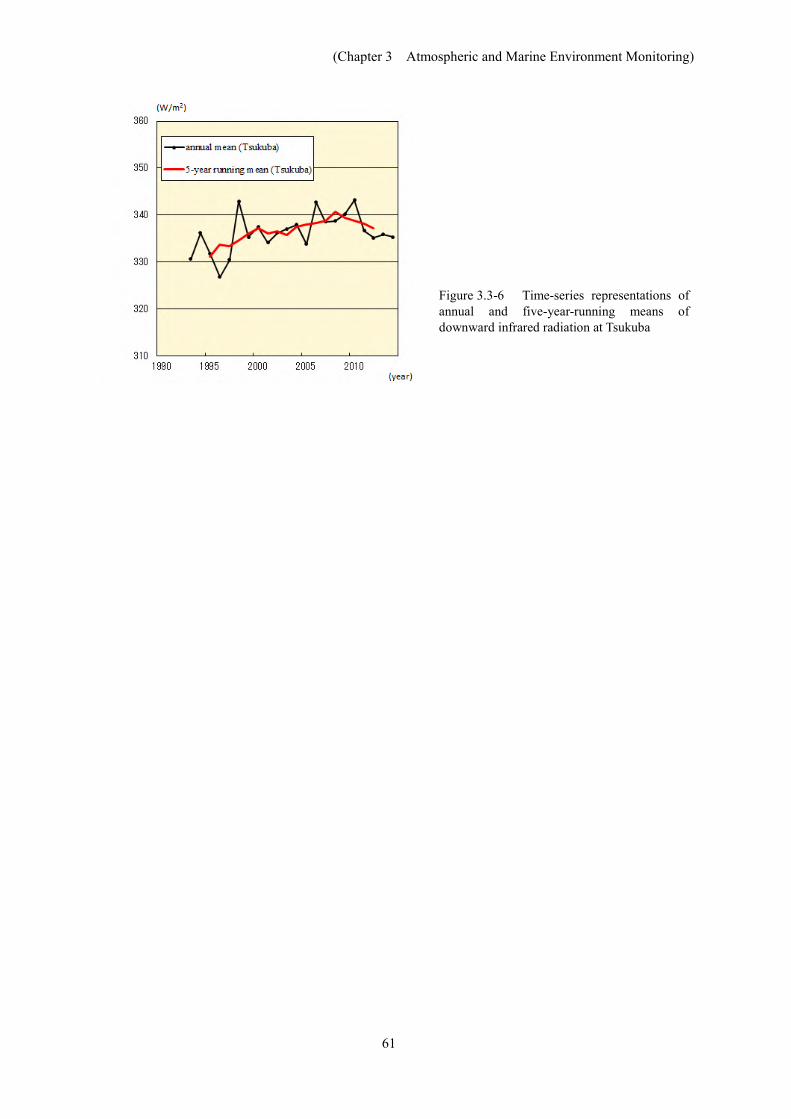
In Japan, downward infrared radiation has been monitored since the early 1990s at Tsukuba. Analysis of the data obtained shows an increasing trend at a rate of about 0.3 W/m2 per year during the period from 1993 to 2014 (Figure 3.3-6). This is consistent with the trend seen in the results of analysis using data from 20 BSRN37 stations worldwide (+0.3 W/m2 per year during the period from 1992 to 2009) (WCRP, 2010).

37 The BSRN (Baseline Surface Radiation Network) is a global observation network for measuring high-precision surface radiation balance on an ongoing basis. JMA operates five BSRN stations in Japan (Sapporo, Tsukuba, Fukuoka, Ishigakijima and Minamitorishima) and one in Antarctica (Syowa Station).

(Chapter 3 Atmospheric and Marine Environment Monitoring)

61

Figure 3.3-6 Time-series representations of annual and five-year-running means of downward infrared radiation at Tsukuba