Chapter 3

Advection algorithms I. The basics

Numerical solutions to (partial) differential equations always require discretization of the prob-lem. This means that instead of a continuous space dimension x or time dimension t we nowhave:

x ! xi " {x1, · · · , xNx} (3.1)t ! tn " {t1, · · · , xNt} (3.2)

In other words: we have replaced spacetime with a discrete set of points. This is called a gridor a mesh. The numerical solution is solved on these discrete grid points. So we must replacefunctions such as q(x) or q(x, t) by their discrete counterparts q(xi) or q(xi, tn). From now onwe will write this as:

q(xi, tn) =: qni (3.3)

NOTE: The upper index of qn is not a powerlaw index, but just the time index. We must nowreplace the partial differential equation also with a discretized form, with qn

i as the quantities wewish to solve. In general we with to find qn+1

i for given qni , so the equations must be formulated in

the way to yield qn+1i for given qn

i . There are infinite ways to formulate the discretized form of thePDEs of hydrodynamics, and some formulations are better than others. In fact, as we shall findout, the simplest formulations tend to be even numerically unstable. And many stable algorithmsturn out to be very diffusive. The art of numerical hydrodynamics, or of numerical solutions toPDEs in general, is to formulate a discretized form of the PDEs such that the solutions for qn

i forgiven initial condition q1

i are numerically stable and are as close as possible to the true q(xi, tn).Over the past 40 years this has turned out to be a very challenging problem, and even to this dayresearch is on-going to design even better methods than before. One of the main problem is thatthere is no ideal and universally good method. Some problems require entirely different methodsthan others, even though they solve exactly the same equations. For example: hydrodynamics ofvery subsonic flows usually requires different methods than hydrodynamics of superonic flowswith shock waves. In the first case we require higher-order precision algorithms while in thesecond case we need so-called shock-capturing methods. We will discuss such methods in laterchapters.

In this chapter we will focus our attention to the fundamental and easy to formulate problemof numerical advection on a grid. As we have seen in Chapter 2, the equations of hydrodynamicscan be reduced to signals propagating with three different speeds: the two sound waves and thegas motion. These ‘signals’ are nothing else than the eigenvectors of the Jacobian matrix, andare therefore combinations of !, !u and !etot, or in other words the eigenvector decomposition

37

38

coefficients (q̃1, q̃2, q̃3). So it should be possible to formulate numerical hydrodynamics as anumerical advection of these signals over a grid.

To simplify things we will not focus on the full set of signals. Instead we focus entirely onhow a scalar function q(x, t) can be numerically advected over a grid. The equation is simply:

"tq(x, t) + "x[q(x, t)u(x, t)] = 0 (3.4)

which is the conserved advection equation. This problem sounds nearly trivial, but it is far fromtrivial in practice. In fact, finding a proper algorithm for numerical advection of scalar functionsover a grid has been one of the main challenges for numerical hydrodynamics in the early yearsof hydrodynamics. We will in fact reduce the complexity of the problem even further and studysimply:

"tq(x, t) + u"x[q(x, t)] = 0 (3.5)

with u is a constant. In this case the equation is automatically a conservation equation in spite ofthe fact that u is outside of the differential operator.

Since not all readers may be familiar with numerical methods, we will start this chapterwith a recapitulation of some basic methods for the integration of functions.

3.1 Prelude: Numerical integration of an ordinary differential equationIn spite of its simplicity, the advection equation is a 2-D problem (in x, t) which therefore alreadynaturally has some level of complexity. To introduce some of the basic concepts that we can uselater, we first turn our attention to a simple problem: the solution to an ordinary differentialequation (ODE) such as

dq(t)

dt= F (t, q(t)) (3.6)

where F (t, q) is a function of both t and q. We assume that at some time t = t0 we know thevalue of q and we wish to integrate this equation in time t using a numerical method. To do thiswe must discretize time t in discrete steps t0, t1, t2 etc, and the values of q(t) belonging to thesetime nodes can be denoted as q0, q1, q2 etc. So, given q0, how can we compute qi with i > 0?The most straightforward method is the forward Euler method:

qn+1 # qn

!t= F (tn, qn) (3.7)

which can be written as an expression for qn+1:

qn+1 = qn + F (tn, qn)!t (3.8)

This method is also called explicit integration, because the new value of q is explicitly given interms of the old values. This is the easiest method, but it has several drawbacks. One of thesedrawbacks is that it becomes numerically unstable if the time step !t is taken too large.! Exercise: Consider the equation

dq(t)

dt= #q(t)2 (3.9)

Write down the analytic solution (to later compare with). Assume q(t = 0) = 1 andnumerically integrate this equation using the forward Euler method to time t = 10. Plot

39

the numerical resulting function q(t) over the analytic solution. Experiment with differenttime steps !t, and find out what happens when !t is taken too large. Derive a reasonablecondition for the maximum !t that can be allowed. Find out which !t is needed to getreasonable accuracy.A way to stabilize the integration even for very large time steps is to use the backward Euler

method:qn+1 = qn + F (tn+1, qn+1)!t (3.10)

which is also often called implicit integration. This equation may seem like magic, because tocalculate qn+1 we need qn+1 itself! The trick here is that one can often manipulate the equationsuch that in the end qn+1 is written in explicit form again. For instance:

dq(t)

dt= #q (3.11)

discretizes implicitly toqn+1 = qn # qn+1!t (3.12)

While this is an implicit equation, one can rewrite it to:

qn+1 =qn

1 + !t(3.13)

which is stable for all !t > 0. However, in many cases F (t, q) is non-linear, and this simplemanipulation is not possible. In that case one is either forced to linearize the equations about thecurrent value of qn and perform the manipulations with #qn+1/2 $ qn+1#qn, or one uses iteration,in which a first guess is made for qn+1 and this is re-computed iteratively until convergence. Thelatter method is, however, rather time-consuming.

Whether implicit methods produce accurate results for large !t is another issue. In fact,such implicit integration, while being numerically extraordinarily stable, is about as inaccurateas explicit integration.

An alternative method, that combines the ideas of both forward and backward Euler inte-gration is the midpoint rule:

qn+1 = qn + F (tn+1/2, qn+1/2)!t (3.14)

where n + 1/2 stands for the position between tn and tn+1. Here the problem is that we do notknow qn+1/2, neither currently, nor once we know qn+1. For problems of integrating Hamiltoniansystems this method can nevertheless work and turns out to be very useful. This is because the’coordinates’ qi are located at tn and the conjugate momenta pi are located at tn+1/2, and theirtime derivatives only depend on their conjugate (q on p and p on q). This forms the basis ofsymplectic integrators such as the leapfrog method.

An integration method very akin to the midpoint rule, but more readily applicable is thetrapezoid rule:

qn+1 = qn +1

2[F (tn, qn) + F (tn+1, qn+1)]!t (3.15)

It is half-implicit. For the above simple example (Eq. 3.11) we can thus write:

qn+1 = qn #1

2qn!t #

1

2qn+1!t (3.16)

40

which results in:qn+1 =

1 # !t/2

1 + !t/2qn (3.17)

This method, when generalized to multiple dimensional partial differential equations, is calledthe Crank-Nicholson method. It has the advantage that it is usually numerically stable (thoughnot as stable as fully implicit methods) and since the midpoint is used, it is also naturally moreaccurate. A variant of this method is the predictor-corrector method (or better: the most well-known of the predictor-corrector methods) in which a temporate prediction of qn+1 is made withthe explicit forward Euler method, which is then used as the qn+1 in the trapezoid rule.

So far we have always calculated qn+1 on the basis of the known qn (and, in case of implicitschemes, on qn+1 as well). Such methods are either first order accurate (such as the forwardand backward Euler methods) or second order accurate (such as the trapezoid rule), but they cannever be of higher order. However, there exist higher-order methods for integration. They eithermake predictor-steps in between tn and tn+1 (these are the Runge-Kutta type methods) or they fita Lagrange polynomial through qn, qn!1 (or even qn!2 and further) to compute the integral of theODE in the interval [tn, tn+1] for finding qn+1 (these are Adams-Bashforth methods). The firstorder Adams method is equal to the forward Euler method. The second and third order ones are:

qn+1 = qn +!t

2[3F (tn, qn) # F (tn!1, qn!1)] (3.18)

qn+1 = qn +!t

12[23F (tn, qn) # 16F (tn!1, qn!1) + 5F (tn!2, qn!2)] (3.19)

However, when generalized to multi-dimensional systems (such as hydrodynamics equations)such higher order multi-point schemes in time are not very often used. In astrophysics thePENCIL hydrodynamics code is a code that uses higher order Runge-Kutta type integrationin time, but most astrophysical codes are first or second order in time.

3.2 Numerical spatial derivatives3.2.1 Second order expressions for numerical spatial derivativesTo convert the PDEs of Eqs. (3.4,3.5) into a discrete form we need to formulate the derivativesin discrete form. A derivative is defined as:

"q

"x= lim

!x"0

q(x + !x) # q(x)

!x(3.20)

For!xwe could take xi+1#xi, but in a numerical calculation we cannot do the lim!x"0 becauseit would require infinite number of grid points. So the best we can do is write:

"q

"x

!

!

!

!

i+1/2

=qi+1 # qi

xi+1 # xi+ O(!x2) %

qi+1 # qi

xi+1 # xi(3.21)

where!x $ (xi+1 #xi), and we assume for the moment that the grid is constantly spaced. Notethat this is an approximate expression of the derivative defined in between the grid points xi+1

and xi. For this reason we denote this as the derivative at i + 1/2, which is just a way to indexlocations in-between grid points. Often one needs the derivative not in between two grid points(i + 1/2), but precisely at a grid point (i). This can be written as:

"q

"x

!

!

!

!

i

=qi+1 # qi!1

xi+1 # xi!1+ O(!x2) %

qi+1 # qi!1

xi+1 # xi!1(3.22)

41

So depending where we need the derivative, we have different expressions for them.TheO(!x2) in Eqs. (3.21, 3.22) is a way of writing the deviation between the ‘true’ deriva-

tive and the approximation. Of course, the true derivative is only defined as long as q(x) issmoothly defined. In our numerical algorithm we do not have q(x): we only have qi, and hencethe ‘true’ derivative is not defined. But it does show that if we re-express the whole problem ona finer grid, i.e. with smaller!x, then the approximate answer approaches the true one as!x2.

To see this, we assume we know the smooth function q(x). We say that qi = q(xi) andqi+1 = q(xi+1) = q(xi + !x) and we express q(xi + !x) as a Taylor series:

q(xi + !x) = q(xi) + q#(xi)!x +1

2q##(xi)!x2 +

1

6q###(xi)!x4 + O(!x4) (3.23)

where the # (prime) denotes the derivative to x. Then we insert this into the numerical derivativeat i:qi+1 # qi!1

2!x=

qi + q#i!x + 12q

##i !x2 + 1

6q###i !x3 + · · ·# qi + q#i!x # 1

2q##i !x2 + 1

6q###i !x3 + · · ·

2!x

= q#i +1

6q###i !x2 + · · ·

(3.24)

This shows that the deviations are of order O(!x2).

3.2.2 Higher-order expressions for numerical derivativesThe O(!x2) also shows that there must be various other expressions possible for the derivativethat are equally valid. Eq. 3.21 is an example of a two-point derivative at position i + 1/2.Eq. 3.22 is also a two-point derivative, this time at position i, but it is defined on a three-pointstencil. A stencil around point i is a mini-grid of points that contribute to the things we wish toevaluate at i. We can also define a derivative at i on a five-point stencil:

"q

"x

!

!

!

!

i

=#qi+2 + 8qi+1 # 8qi!1 + qi!2

12!x+ O(!x4) (3.25)

Note: this expression is only valid for a constantly-spaced grid!! Exercise: Show that this expression indeed reproduces the derivative to order O(!x4).

Some hydrodynamics codes are based on such higher-order numerical derivatives. Collo-quially it is usually said that higher-order schemes are more accurate than lower-order schemes.However, this is only true if the function q(x) is reasonably smooth over length scales of order!x. In other words: the O(!x4) is only significantly smaller than O(!x2) if "5

xq(x)!x4 &"3

xq(x)!x2 & "xq(x). Higher-order schemes are therefore useful for flows that have no strongdiscontinuities in them. This is often true for subsonic flows, i.e. flows for which the sound speedis much larger than the typical flow speeds. For problems involving shock waves and other typesof discontinuities such higher-order schemes turn out to be worse than lower order ones, as wewill show below.

3.3 Some first advection algorithmsIn this section we will try out a few algorithms and find out what properties they have. We focusagain on the advection equation

"tq + u"xq = 0 (3.26)

42

Figure 3.1. Result of center-difference algorithm for advection of a step-function from left toright. Solid line and symbols: numerical result. Dotten line: true answer (produced analyti-cally).

with constant u > 0. The domain of interest is [x0, x1]. We assume that the initial state q(x, t =t0) is given on this domain, and we wish to solve for q(x, t > t0). A boundary condition has tobe specified at x = x0.

3.3.1 Centered-differencing schemeThe simplest discretization of the equation is:

qn+1i # qn

i

tn+1 # tn+ u

qni+1 # qn

i!1

xi+1 # xi!1= 0 (3.27)

in which we use the n + 1/2 derivative in the time direction and the i derivative in space. Letus assume that the space grid is equally-spaced so that we can always write xi+1 # xi!1 = 2!x.We can then rewrite the above equation as:

qn+1i = qn

i #!t

2!xu(qn

i+1 # qni!1) (3.28)

This is one of the simplest advection algorithms possible.Let us test it by applying it to a simple example problem. We take x0 = 0, x1 = 100 and:

q(x, t = t0) =

"

1 for x ' 300 for x > 30

(3.29)

As boundary condition at x = 0 we set q(x = 0, t) = 0. Let us use an x-grid with spacing!x =1, i.e. we have 100 grid points located at i + 1/2 for i " [0, 99]. Let us choose !t $ tn+1 # tnto be !t = 0.1!x for now. If we do 300 time steps, then we expect the jump in q to be locatedat x = 60. In Fig. 3.1 we see the result that the numerical algorithm produces.

One can see that this algorithm is numerically unstable. It produces strong oscillations inthe downsteam region. For larger !t these oscillations become even stronger. For smaller !tthey may become weaker, but they are always present. Clearly this algorithm is of no use. Weshould find a better method

43

Figure 3.2. Result of center-difference algorithm for advection of a step-function from left toright. Solid line and symbols: numerical result. Dotten line: true answer (produced analyti-cally).

3.3.2 Upstream(Upwind) differencingOne reason for the failure of the above centered-difference method is the fact that the informa-tion needed to update qn

i in time is derived from values of q in both upstream and downstreamdirections1. The upstream direction at some point xi is the direction x < xi (for u > 0) sincethat is the direction from which the flow comes. The downsteam direction is x > xi, i.e. thedirection where the stream goes. Anything that happens to the flow downstream from xi shouldnever affect the value of q(xi), because that information should flow further away from xi. Thisis because, by definition, information flows downstream. Unfortunately, for the centered dif-ferencing scheme, information can flow upstream: the value of qn+1

i depends as much on qni+1

(downstream direction) as it does on qni!1 (upstream direction). Clearly this is unphysical, and

this is one of the reasons that the algorithm fails.A better method is, however, easily generated:

qn+1i # qn

i

tn+1 # tn+ u

qni # qn

i!1

xi # xi!1= 0 (3.30)

which is, by the way, only valid for u > 0. In this equation the information is clearly onlyfrom upstream to downstream. This is called upstream differencing, often also called upwinddifferencing. The update for the state is then:

qn+1i = qn

i #!t

!xu(qn

i # qni!1) (3.31)

If we now do the same experiment as before we obtain the results shown in Figure 3.2.This looks already much better. It is not unstable, and it does not produce values larger thanthe maximum value of the initial state, nor values smaller than the minimal value of the initialstate. It is also monotonicity preserving, meaning that it does not produce new local minimaor maxima. However, the step function is smeared out considerably, which is an undesirableproperty.

1These are also often called upwind and downwind directions.

44

x

t

ii−1i−2 i+1 i+2

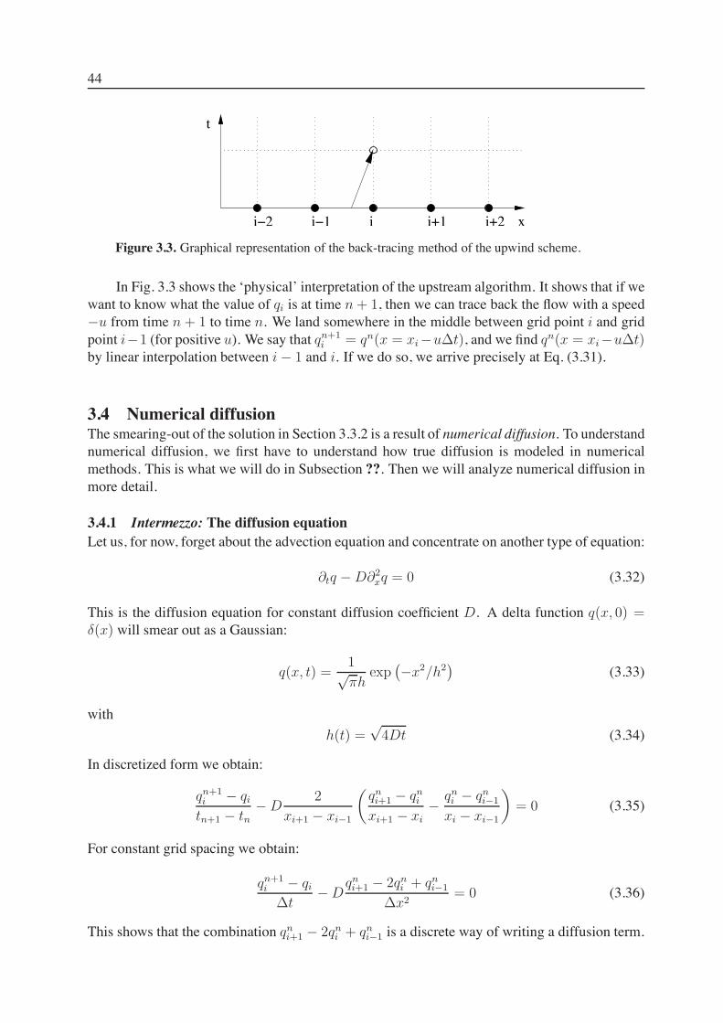
Figure 3.3. Graphical representation of the back-tracing method of the upwind scheme.

In Fig. 3.3 shows the ‘physical’ interpretation of the upstream algorithm. It shows that if wewant to know what the value of qi is at time n + 1, then we can trace back the flow with a speed#u from time n + 1 to time n. We land somewhere in the middle between grid point i and gridpoint i#1 (for positive u). We say that qn+1

i = qn(x = xi#u!t), and we find qn(x = xi#u!t)by linear interpolation between i # 1 and i. If we do so, we arrive precisely at Eq. (3.31).

3.4 Numerical diffusionThe smearing-out of the solution in Section 3.3.2 is a result of numerical diffusion. To understandnumerical diffusion, we first have to understand how true diffusion is modeled in numericalmethods. This is what we will do in Subsection ??. Then we will analyze numerical diffusion inmore detail.

3.4.1 Intermezzo: The diffusion equationLet us, for now, forget about the advection equation and concentrate on another type of equation:

"tq # D"2xq = 0 (3.32)

This is the diffusion equation for constant diffusion coefficient D. A delta function q(x, 0) =#(x) will smear out as a Gaussian:

q(x, t) =1($h

exp#

#x2/h2$

(3.33)

withh(t) =

(4Dt (3.34)

In discretized form we obtain:

qn+1i # qi

tn+1 # tn# D

2

xi+1 # xi!1

%

qni+1 # qn

i

xi+1 # xi#

qni # qn

i!1

xi # xi!1

&

= 0 (3.35)

For constant grid spacing we obtain:

qn+1i # qi

!t# D

qni+1 # 2qn

i + qni!1

!x2= 0 (3.36)

This shows that the combination qni+1 # 2qn

i + qni!1 is a discrete way of writing a diffusion term.

45

3.4.2 Numerical diffusion of advection algorithmsSo now let us go back to the pure advection equation. Even though this equation does not haveany diffusion in it, the numerical algorithm to solve this advection equation intrinsically hassome diffusion. In fact, there exists no numerical method without numerical diffusion. Somealgorithms have more of it, some have less, and there exist method to constrain the smearing-out of discontinuities (see Section 4.5 on flux limiters). But in principle numerical diffusion isunavoidable.

One way of seeing this is by doing the following exercise. Consider the upwind scheme. Ituses the derivative i# 1/2 for the update of the state at i. In principle this is a bit cheating, sinceone ‘should’ use the i derivative for the update at i. So let us write the derivative at i # 1/2 as:

qi # qi!1

!x=

qi+1 # qi!1

2!x# !x

qi+1 # 2qi + qi!1

2!x2(3.37)

The left-hand-side is the upstream difference, the first term on the right-hand-side is the centereddifference and the second term on the right-hand-side can be recognized as a diffusion term withdiffusion constant

D =!xu

2(3.38)

This shows that the upstream difference scheme can be regarded to be the same as the centereddifference scheme supplemented with a diffusion term. The pure centered difference schemeis unstable, but once a bit of diffusion is added, the algorithm stabilizes. The drawback is,however, that the diffusion smears any features out. If one would define the centered differenceformulation of the x-derivative as the ‘true’ derivative (which is of course merely a definition),then the numerical diffusion of the upstream differencing scheme is quantified by D as given inEq. (3.38).

In practice it is not possible to perfectly define the diffusivity of an algorithm since thecentered difference formulation of the derivative is also merely an approximation of the truederivative. But it is nevertheless a useful way of looking at the concept of numerical diffusion.In principle one could say that it is as if we are solving

"tq + u"xq #!xu

2"2

xq = 0 (3.39)

Clearly, for !x ! 0 the diffusion vanishes. This is obviously a necessary condition, otherwisewe would be modeling the true diffusion equation, which is not what we want. The diffusionthat we see here is merely a by-product of the numerical algorithm we used.

Note that sometimes (as we shall see below) it is useful to add some viscosity on purposeto an algorithm. This is called artificial viscosity. One could therefore say that the upstreamdifferencing is equal to centered differencing plus artificial viscosity.

3.5 Courant-Friedichs-Lewy conditionNo matter how stable an explicit numerical algorithm is, it cannot work for arbitrarily large timestep !t. If, in the above example (with !x = 1 and u = 1), we were to use the upstreamdifferencing method but we would take !t = 2, then the algorithm would produce completelyunstable results. The reason is the following: The function q is advected over a distance of u!tin a time step !t. If u!t > !x, then within a single time step the function is advected over alarger distance than the grid spacing. However, with the above upstream differencing method the

46

new qn+1i depends only on the old qn

i!1 and qni values. The algorithm does not include information

about the value of qni!2, but with such a large !t it should have included it. The algorithm does

not know (at least within a single time step) about qni!2 and therefore it produces something that

is clearly not a solution.To keep a numerical algorithm stable the time step has to obey the Courant-Friedrichs-Lewy

condition (CFL condition) which states that the domain of dependence of qn+1i of the algorithm

at time t = tn should include the true domain of dependence at time t = tn. Or in otherwords: nothing is allowed to flow more than 1 grid spacing within one time step. This meansquantitatively

!t '!x

u(3.40)

So the higher the velocity u, the smaller the maximum allowed time step.For the case that u ! u(x) (i.e. space-dependent velocity) this gives different time step

constraints at different locations. The allowed global time step is then the smallest of these.Not always one wants to take this maximum allowed time step. Typically one takes:

!t = C min(!x/u) (3.41)

where C is the Courant number. If one takes this 1, then one takes the maximum allowed timestep. If it is 0.5 then one takes half of it.

The CFL condition is a nessecary (but not sufficient) condition for the stability of any ex-plicit differencing method. All the methods we have discussed here, and most of the methodswe will discuss lateron, are explicit differencing methods. The work ‘explicit’ points to the factthat the updated state qn+1

i is explicitly formulated in terms of qni±k. There exist also so called

‘implicit differencing’ methods, but they are often too complex and therefore less often used.

3.6 Local truncation error and order of the algorithmNow that we have seen some of the basics of numerical advection algorithms, let us analyzehow accurate such algorithms are. Let us define qe(x, t) to be an exact solution to the advectionequation and qn

i a discrete solution to the numerical advection equation. The numerical algorithmwill be represented by a transport operator T :

qn+1i = T [qn

i ] (3.42)

which is another way of writing the discretized PDE. In case of the upstream differencing methodwe have T [qn

i ] = qni # !t

!xu(qni # qn

i!1) (cf. Eq. 3.31). For this method the T operator is a linearoperator. Note, incidently, that if the PDE is a linear PDE, that does not guarantee that thetransport operator T is also necessarily linear. Lateron in this chapter we will get to know non-linear operators that represent linear PDEs.

We can also define the discrete values of the exact solution:

qne,i $ qe(xi, tn) (3.43)

The values qne,i do not in general strictly obey Eq. (3.42). But we can apply the operator T to qn

e,i

and compare to qn+1e,i . In other words: we can see which error the discrete operator T introduces

in one single time step compared to the true solution qn+1e,i . So let us apply T to qn

e,i and definethe one step error (OSE) as follows:

OSE = T [qne,i] # qn+1

e,i (3.44)

47

By using a Taylor expansion we can write qn+1e,i as:

qn+1e,i = qn

e,i +

%

"q(xi, t)

"t

&

t=tn

!t +1

2

%

"2q(xi, t)

"t2

&

t=tn

!t2 + O(!t3) (3.45)

If we use the upstream difference scheme, we can write:

T [qne,i] = qn

e,i #!t

!xu(qn

e,i # qne,i!1) (3.46)

where we can write:

qne,i!1 = qn

e,i #%

"q(x, tn)

"x

&

x=xi

!x +1

2

%

"2q(x, tn)

"x2

&

x=xi

!x2 + O(!x3) (3.47)

So the OSE of this scheme becomes:

OSE = # u

%

"q(x, tn)

"x

&

x=xi

!t +1

2u

%

"2q(x, tn)

"x2

&

x=xi

!t!x + u!tO(!x2)#%

"q(xi, t)

"t

&

t=tn

!t #1

2

%

"2q(xi, t)

"t2

&

t=tn

!t2 + O(!t3)

(3.48)

If we ignore all terms of higher order we obtain:

OSE = #!t

'

%

"q(xi, t)

"t

&

t=tn

+ u

%

"q(x, tn)

"x

&

x=xi

#O(!t) #O(!x)

(

(3.49)

From the PDE we know that the first two terms between brackets cancel identically, so we obtain:

OSE = !t[O(!t) + O(!x)] (3.50)

So what happens when we make!t smaller: the OSE gets smaller by a factor of!t2. However,one must keep in mind that one now has to do more time steps to arrive at the same simulationend-time. Therefore the final error goes down only as!t, i.e. linear instead of quadratic. That iswhy it is convenient if we define the so-called local truncation error (LTE) as:

LTE $1

!t(T [qn

e,i] # qn+1e,i ) (3.51)

which for this particular scheme is:

LTE = O(!t) + O(!x) (3.52)

In general an algorithm is called consistent with the partial differential equation when theLTE behaves as:

LTE =)

k=0,l

O(!tk!xl!k) (3.53)

with l ' 1. The LTE is of order l, and the algorithm is said to be l-th order.The upstream differencing algorithm is clearly a first order scheme.

48

3.7 Lax-Richtmyer stability analysis of numerical advection schemesThe mere fact that the LTE goes withO(!t) andO(!x) is not a sufficient condition for stability.It says that the operator T truly describes the discrete version of the PDE under consideration.But upon multiple successive actions of the operator T , representing the time sequence of thefunction q, tiny errors could conceivably grow exponentially and eventually dominate the solu-tion. We want to find out under which conditions this happens.

To analyze stability we need to first define what we mean by stability. To do this we mustdefine a norm ||.|| by which we can measure the magnitude of the error. In general we define thep-norm of a function E(x) as:

||E||p =

%* $

!$

|E(x)|pdx

&1/p

(3.54)

For the discretized function Ei this becomes:

||E||p =

+

!x$

)

i=!$

|Ei|p,1/p

(3.55)

The most commonly used are the 1-norm and the 2-norm. For conservation laws the 1-norm isattractive because this norm can be directly used to represent the conservation of this quantity.However, the 2-norm is useful for linear problems because it is compatible with a Fourier analysisof the problem (see Section 3.8).

Now suppose we start at t = 0with a function qe(x, t = 0) and we set the discrete numericalsolution at that time to these values: q0

i = q0e,i $ qe(xi, 0). The evolution in time is now given by

a successive application of the operator T , such that at time t = tn the discrete solution is:

qni = T n[q0

i ] (3.56)

In each of these time steps the discrete solution acquires an error. We can write the total accu-mulated global error at time t = tn as En

i defined as:

Eni = qn

i # qne,i (3.57)

i.e. the difference between the discrete solution and the true solution. So when we apply theoperator T to qn

i we can write:

qn+1i $ T [qn

i ] = T [qne,i + En

i ] (3.58)

So we can now write the global error at time tn+1, En+1i as

En+1i = qn+1

i # qn+1e,i

= T [qne,i + En

i ] # qn+1e,i

= T [qne,i + En

i ] # T [qne,i] + T [qn

e,i] # qn+1e,i

= T [qne,i + En

i ] # T [qne,i] + !tLTE[qn

e,i]

(3.59)

Now in the next few paragraphs we will show that the numerical method is stable in somenorm ||.|| if the operator T [] is a contractive operator, defined as an operator for which

||T [P ] # T [Q]|| ' ||P # Q|| (3.60)

49

for any functions P and Q. To show this we write

||En+1|| ' ||T [qne + En] # T [qn

e ]|| + !t||LTE[qne ]||

' ||En|| + !t||LTE[qne ]||

(3.61)

If we apply this recursively we get

||EN || ' !tN

)

n=1

||LTE[qne ]|| (3.62)

where we assume that the error at t = t0 = 0 is zero. Now, the LTE is defined always on the truesolution qn

e,i. So since the true solution is for sure well-behaved (numerical instabilities are onlyexpected to arise in the numerical solution qn

i ), we expect that the ||LTE[qne ]|| is a number that

is bounded. If we defineMLTE to be

MLTE = max1%n%N ||LTE[qne ]|| (3.63)

which is therefore also a bound number (not suject to exponential growth), then we can write:

||EN || ' N!tMLTE (3.64)

or with t = N!t:||EN || ' tMLTE (3.65)

This shows that the final global error is bound, i.e. not subject to run-away growth, if the operatorT is contractive. Note that this analysis, so far, holds both for linear operators T [.] as well as fornon-linear operators T [.]. We will cover non-linear operators in the next chapter.

If T [.] is linear one can write T [qne + En] # T [qn

e ] = T [En]. In this case the stabilityrequirement is:

||T [En]|| ' ||En|| (3.66)

which must be true for any function Eni . In Section 3.8 we will verify this for some simple

algorithms.Sometimes the above stability requirement is loosened a bit. The idea behind this is that we

are not concerned if modes grow very slowly, as long as these modes do not start to dominatethe solution. If the operator T [.] obeys

||T [P ] # T [Q]|| ' (1 + %!t)||P # Q|| (3.67)

where % is some constant (which we will constrain later), then Eq.(3.61) becomes:

||En+1|| ' (1 + %!t) ||En|| + !t||LTE[qne ]|| (3.68)

and thereby Eq.(3.65) becomes:||EN || ' tMLTEe!t (3.69)

One sees that the error growth exponentially in time, which one would in principle consider aninstability. But e!t is a constant that does not depend on !t. So no matter how large e!t is, aslong as the LTE is linear or higher in !t (a requirement for consistency) one can always find a!t small enough such that ||EN || & ||qN

e || even though this might require a very large numberof time steps for the integration. This means that for an operator T [.] obeying Eq.(3.67) the

50

algorithm is formally stable. In practice, of course, the % cannot be too large, or else one wouldrequire too many time steps (i.e. too small!t) to be of any practical use.

This leads us to a fundamental theorem of numerical integration methods: Lax EquivalenceTheorem which says that:

Consistency + Stability ! Convergence

In other words: if an algorithm is consistent (see Eq.3.53) and stable (see Eq.3.69), then one canbe assured that one can find a small enough !t such that at time t the right answer is reacheddown to an accuracy of choice.

3.8 Von Neumann stability analysis of numerical advection schemesThe theoretical stability analysis outlined in the previous section has only reformulated the condi-tion for stability as a condition on the operator T [.]. We now analyze whether a certain algorithmin fact satisfies this condition. For linear operators the Von Neumann analysis does this in Fourierspace using the 2-norm. Also we will require strong stability, in the sense that we want to showthat ||T [En]|| ' ||En|| (i.e. without the (1 + %!t) factor).

Any function can be expressed as a sum of complex wave functions. For an infinite spaceone can therefore write the initial condition function q(x) as

q(x) =1(2$

* $

!$

q̃(k)eikxdk (3.70)

Since the advection equation"tq + u"xq = 0 (3.71)

merely moves this function with velocity u, the solution q(x, t) = q(x#ut) translates in a q̃(k, t)given by

q̃(k, t) = q̃(k)e!iukt (3.72)

which is just a phase rotation. In Fourier space, the true operator Te[.] is therefore merely acomplex number: Te = e!iuk!t. As we shall see below, the numerical operator in Fourier spaceis also a complex number, though in general a slightly different one. So we need to comparethe numerical operator T [.] with the true operator Te[.] to find out what the local truncation error(LTE) is.

Formally, when we follow the logic of Section 3.7, we need to let the operator T [.] act onthe Fourier transforms of qn

e,i + Eni and qn

e,i and subtract them. Or since the operator is linear, wemust apply it to the Fourier transform of En

i . However, since we have assumed that the operatoris linear, we can also do the analysis directly on q̃n

e (k) (the Fourier transform of qne,i) and check if

the resulting amplitude is' 1. The advantage is that we can then directly derive the LTE in termsof an amplitude error and a phase error. If the amplitude of the operator T is ' 1 for all valuesof k, !x and !t ' C!x/|u| (where u is the advection speed and C is the Courant number)then we know that the function q̃(k, t) is not growing exponentially, and therefore also the erroris not growing exponentially. Moreover, we know that if this amplitude is much smaller than 1,then the algorithm is very diffusive. We can also analyze the phase error to see if the algorithmtransports each mode with the correct speed.

51

3.8.1 Analyzing the centered differencing schemeLet us descretize this function as:

q0i := q(x = xi, 0) = eikxi (3.73)

Now insert this into the centered difference scheme:

qn+1i = qn

i #!t

2!xu(qn

i+1 # qni!1) (3.74)

We obtain

q1i = eikxi #

!t

2!xu(eik(xi+!x) # eik(xi!!x)) = eikxi

-

1 #!t

2!xu(eik!x # e!ik!x)

.

(3.75)

Let us define:

& $ u!t

!x(3.76)

and' $ k!x (3.77)

then we can writeqn+1i = qn

i TC (3.78)with T T the transfer function, which for centered differencing is apparently

TC = 1 #&

2(ei" # e!i") (3.79)

The C in the transfer function stands for ‘centered differencing’. We can write TC as

TC = 1 # i& sin ' (3.80)

This transfer function is most easily analyzed by computing the squared magnitudeR

R = T &T = (ReT )2 + (ImT )2 (3.81)

and the phase "

tan " =ImT

ReT(3.82)

which for this algorithm are:

RT = 1 + &2 sin2 ' , tan "T = #& sin ' (3.83)

We can now compare this to our analytic solution (the solution that should have been pro-duced): q(x, t) = eik(x!u!t). Clearly this analytic solution has R = 1 and a phase of " = uk!t(if phase is measured negatively). Compared to this solution we see that:1. The centered differencing scheme diverges: the amplitude of the solution always getsbigger. For very small time steps this happens with a factor 1+ (uk!t)2. So clearly it getsbetter for smaller time steps (even if we have to take more of them), but it still remainsunconditionally unstable.

2. The phase also has an error: u#t[sin(k!x) # k!x]/!x. For very small time steps thephase error becomes: #k3u!t!x2/6, which means that the phase error grows linearly intime, independent of!t.

These results confirm our numerical experience that the centered differencing method is uncon-ditionally unstable.

52

3.8.2 Now adding artificial viscosityWe have seen in the numerical experiments of Section 3.3.2 that adding artificial viscosity (seeSection 3.4.2) can stabilize an algorithm. So let us now consider the following advection scheme:

qn+1i = qn

i #!t

2!xu(qn

i+1 # qni!1) + D

!t

!x2(qn

i+1 # 2qni + qn

i!1) (3.84)

Let us define( = D

!t

!x2(3.85)

so that we getqn+1i = qn

i #&

2(qn

i+1 # qni!1) + ((qn

i+1 # 2qni + qn

i!1) (3.86)

Let us again insert q0i := q(x = xi, 0) = eikxi so that we obtain

q1i = eikxi #

&

2(eik(xi+!x) # eik(xi!!x)) + ((eik(xi+!x) # 2eikxi + eik(xi!!x))

= eikxi

/

1 #&

2(eik!x # e!ik!x) + ((eik!x # 2 + e!ik!x)

0 (3.87)

so the transfer function becomes:

TCD = 1 #&

2(eik!x # e!ik!x) + ((eik!x # 2 + e!ik!x) (3.88)

or in other terms:TCD = 1 # i& sin ' + 2((cos' # 1) (3.89)

The R and " are:RCD = &2 sin2 ' + (1 + 2((cos ' # 1))2 (3.90)

andtan "CD = #

& sin '

1 + 2((cos' # 1)(3.91)

Figure 3.4 shows the transfer function in the complex plane. Whenever the transfer functionexceeds the unit circle, the mode grows and the algorithm is unstable. Each of the ellipses showsthe complete set of modes (wavelengths) for a given & and (. None of the points along theellipse is allowed to be beyond the unit circle, because if any point exceeds the unit circle, thenthere exists an unstable mode that will grow exponentially and, sooner or later, will dominate thesolution.

From these figures one can guess that whether an ellipse exceeds the unit circle or not isalready decided for very small ' (i.e. very close to T = 1). So if we expand Eq. (3.90) in ' weobtain

RCD % 1 + '2(&2 # 2() + O('3) (3.92)

We see that for the centered-differencing-and-diffusion algorithm to be stable one must have

( ) &2/2 (3.93)

! Exercise: Argue what is the largest allowed & for which a ( can be found for which allmodes are stable.

53

Figure 3.4. The complex transfer function for the centered differencing advection scheme withadded artificial viscosity (imaginary axis is flipped). The ellipses are curves of constant advec-tion parameter ! = u!t/!x (marked on the curves) and varying " (i.e. varying wavelength).The thick line is the unit circle. Left: # = 0.25, right: # = 0.1. Whenever the transfer functionexceeds the unit circle, the algorithm is unstable since the mode grows.

! Exercise: Analyze the upstream differencing scheme of Section 3.3.2 with the abovemethod,show that it is stable, and derive whether (and if so, how much) this algorithm is more dif-fusive than strictly necessary for stability.

Clearly for ( ) &2/2 the scheme is stable, but does it produce reasonable results? Let us firststudy the phase "CD and compare to the expected value. The expected value is:

" = #uk!t = #&' (3.94)

Comparing this to Eq. (3.91) we see that to first order the phase is OK, at least for small '. Theerror appears when ' gets non-small, i.e. for short wavelength modes. This is not a surprise sinceshort wavelength modes are clearly badly sampled by a numerical scheme.

What about damping? From the phase diagram one can see that if we choose ( largerthan strictly required, then the ellipse moves more to the left, and thereby generally towardsmaller RCD, i.e. strong damping. For small & (assuming we choose ( = &2/2) we see that theellipses flatten. This means that short-wavelength (i.e. large ') modes are strongly damped, andeven longer wavelength modes (the ones that we should be able to model properly) are damped.Since this damping is an exponential process (happening after each time step again, and therebycreating a cumulative effect), even a damping of 10% per time step will result in a damping ofa factor of 10!3 after only 65 time steps. Clearly such a damping, even if it seems not too largefor an individual time step, leads to totally smeared out results in a short time. This is not whatwe would like to have. The solution should, ideally, move precisely along the unit circle, butrealistically this is never attainable. The thing we should aim for is an algorithm that comes asclose as possible to the unit circle, and has an as small as possible error in the phase.

3.8.3 Lax-Wendroff schemeIf we choose, in the above algorithm, precisely enough artificial viscosity to keep the algorithmstable, i.e.

( =1

2&2 (3.95)

54

then the algorithm is called the Lax-Wendroff algorithm. The update for the Lax-Wendroffscheme is evidently:

qn+1i = qn

i #&

2(qn

i+1 # qni!1) +

&2

2(qn

i+1 # 2qni + qn

i!1) (3.96)

Interestingly, the Lax-Wendroff scheme also has another interpretation: that of a predictor-corrector method. In this method we first calculate the qn+1/2

i!1/2 and qn+1/2i+1/2 , i.e. the mid-point

fluxes at half-time:

qn+1/2i!1/2 = 1

2(qni + qn

i!1) + 12&(q

ni!1 # qn

i ) (3.97)

qn+1/2i+1/2 = 1

2(qni + qn

i+1) + 12&(q

ni # qn

i+1) (3.98)

Then we write for the desired qn+1i :

qn+1i = qn

i + &(qn+1/2i!1/2 # qn+1/2

i+1/2 ) (3.99)

Working this out will directly yield Eq. (3.96).

3.9 Phase errors and Godunov’s TheoremThe Lax-Wendroff scheme we derived in the previous section is the prototype of second orderadvection algorithms. There are many more types of second order algorithms, and in the nextchapter we will encounter them in a natural way when we discuss piecewise linear advectionschemes. But most of the qualitative mathematical properties of second order linear schemes ingeneral can be demonstrated with the Lax-Wendroff scheme.

One very important feature of second order schemes is the nature of their phase errors.Using the following Taylor expansions

atanx = x# 13x

3 + O(x4) cosx = 1# 12x

2 + O(x4) sinx = x# 16x

3 + O(x4) (3.100)

we can write the difference "CD # "e:

#"CD $ "CD # "e = #atan

-

& sin '

1 + 2((cos' # 1)

.

+ &'

% &'31

16 # ( + 1

3&22

(3.101)

A phase error can be associated with a lag in space: the wave apparently moves too fast ortoo slow. The lag corresponding to the particular phase error is: #x = #"/k * #"/'. The lagper unit time is then d(#x)/dt = #x/!t * #"/('&). So this becomes

d(#x)

dt* '2

1

16 # ( + 1

3&22

(3.102)

One sees that the spatial lag is clearly dramatically rising when ' ! 1, i.e. for wavelength thatapproach the grid size. In other words: the shortest wavelength modes have the largest error intheir propagation velocity.

Now suppose we wish to advect a block function:

q(x) =

"

1 for x < x0

0 for x > x0(3.103)

55

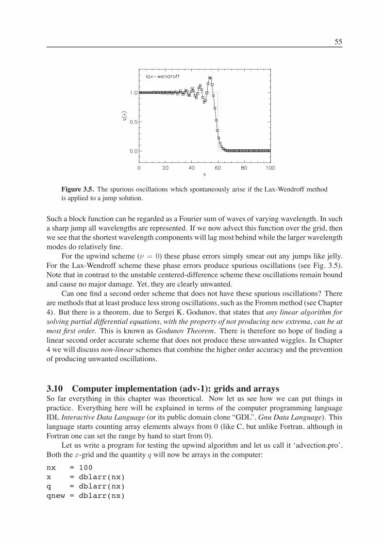
Figure 3.5. The spurious oscillations which spontaneously arise if the Lax-Wendroff methodis applied to a jump solution.

Such a block function can be regarded as a Fourier sum of waves of varying wavelength. In sucha sharp jump all wavelengths are represented. If we now advect this function over the grid, thenwe see that the shortest wavelength components will lag most behind while the larger wavelengthmodes do relatively fine.

For the upwind scheme (( = 0) these phase errors simply smear out any jumps like jelly.For the Lax-Wendroff scheme these phase errors produce spurious oscillations (see Fig. 3.5).Note that in contrast to the unstable centered-difference scheme these oscillations remain boundand cause no major damage. Yet, they are clearly unwanted.

Can one find a second order scheme that does not have these spurious oscillations? Thereare methods that at least produce less strong oscillations, such as the Frommmethod (see Chapter4). But there is a theorem, due to Sergei K. Godunov, that states that any linear algorithm forsolving partial differential equations, with the property of not producing new extrema, can be atmost first order. This is known as Godunov Theorem. There is therefore no hope of finding alinear second order accurate scheme that does not produce these unwanted wiggles. In Chapter4 we will discuss non-linear schemes that combine the higher order accuracy and the preventionof producing unwanted oscillations.

3.10 Computer implementation (adv-1): grids and arraysSo far everything in this chapter was theoretical. Now let us see how we can put things inpractice. Everything here will be explained in terms of the computer programming languageIDL Interactive Data Language (or its public domain clone “GDL”, Gnu Data Language). Thislanguage starts counting array elements always from 0 (like C, but unlike Fortran, although inFortran one can set the range by hand to start from 0).

Let us write a program for testing the upwind algorithm and let us call it ‘advection.pro’.Both the x-grid and the quantity q will now be arrays in the computer:nx = 100x = dblarr(nx)q = dblarr(nx)qnew = dblarr(nx)

56

We can produce a regular grid in x in the following way

dx = 1.d0 ; Set grid spacingfor i=0,nx-1 do x[i] = i*dx

In IDL this can be done even easier with the command dindgen, but let us ignore this for themoment. Now let us put some function on the grid:

for i=0,nx-1 do if x[i] lt 30. then q[i]=1.d0 else q[i]=0.d0

Now let us define a velocity, a time step and a final time:

u = 1.d0dt = 2d-1tend = 30.d0

As a left boundary condition (since u > 0) we can take

qleft = q[0]

Now the simple upwind algorithm can be done for grid point i=1,nx-1:

time = 0.d0while time lt tend do begin

;;;; Check if end time will not be exceeded;;if time + dt lt tend then begin

dtused = dtendif else begin

dtused = tend-timeendelse;;;; Do the advection;;for i=1,nx-1 do begin

qnew[i] = q[i] - u * ( q[i] - q[i-1] ) * dtused / dxendfor;;;; Copy qnew back to q;;for i=1,nx-1 do begin

q[i] = qnew[i]endfor;;;; Set the boundary condition at left side (because u>0);; (Note: this is not explicitly necessary since we;; didn’t touch q[0]);;q[0] = qleft

57

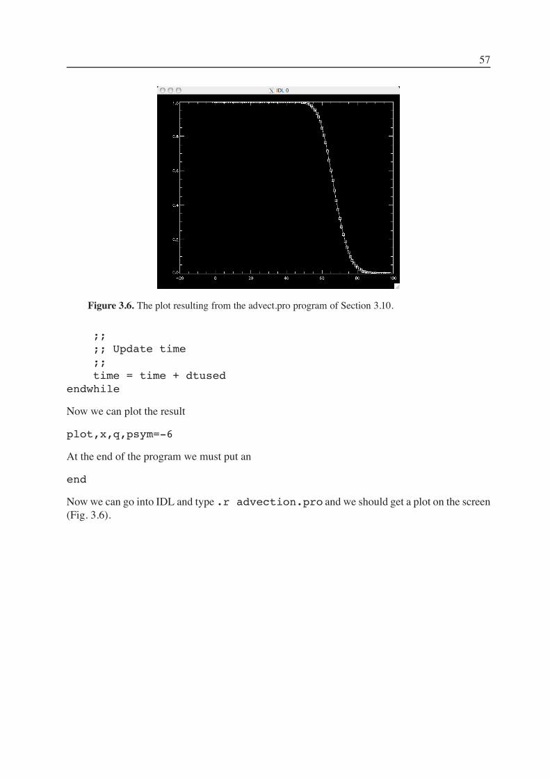
Figure 3.6. The plot resulting from the advect.pro program of Section 3.10.

;;;; Update time;;time = time + dtused

endwhile

Now we can plot the result

plot,x,q,psym=-6

At the end of the program we must put an

end

Nowwe can go into IDL and type .r advection.pro and we should get a plot on the screen(Fig. 3.6).