79

CHAPTER-3

Adsorption studies on fruits of Gular (Ficus glomerata): Removal of Cr(VI) from synthetic wastewater

80

3.1. Introduction

Heavy metals in a water system are hazardous to the environment and

humans due to the bio-accumulation through the food chain and persistence in nature.

Among all heavy metals, copper chromium and zinc ingestion beyond permissible

quantities causes various chronic disorders [1]. Chromium and its compounds are

generally released from electroplating, leather tanning, cement, dyeing, fertilizer,

photography, paint and pigments, textile, steel fabrication, and canning industries.

Cr(III) and Cr(VI) are two stable oxidation states of chromium that persist in

the environment [2]. The trivalent chromium is essential in human nutrition especially

in glucose metabolism while most of the hexavalent compounds of chromium are

toxic to animals, humans and bacteria and are known to be carcinogenic [3,4].The

maximum concentration limit of hexavalent chromium for discharge into inland

surface waters is 0.1mg L-1 and in potable water it is 0.05mg L-1[5].

Many technologies adopted for the removal of chromium from industrial

wastewaters include precipitation, membrane filtration, solvent extraction with

amines; ion-exchange, activated carbon adsorption, electro-deposition, and various

biological processes [6-11]. Most of these methods suffer set-backs because of high

capital and operational cost and lack of skilled personnel problem. Adsorption process

has been extensively used for the removal of toxic metals. Recently various low cost

adsorbents such as agriculture wastes and activated carbon prepared from agriculture

wastes have been used for the removal of toxic metals from aquatic environment [12-

16], where as lichen (Parmilina tiliaceae)[17], banana peel [18], tamarind seeds[19],

pomegranate husk carbon[20], sunflower (Helianthus annuus) stem[21], rice

81

straw[22], Ficus religiosa leaf powder[23], spent activated clay [24], have been used

for the removal Cr(VI) from water and wastewater.

In present study fruits of Ficus glomerata have been used as a new low cost

adsorbent for the removal of Cr(VI) from wastewater. Ficus tree (Ficus glomerata)

belongs to Moraceae family. It is 30-50 feet high and found in northern parts of India

.This tree has auspicious position and forms a major part of worship religious

festivals. The Ficus fruit is 2 inch in diameter. Fruits are green in colour when unripe

and are found in groups. The fruition period is from March to June. The tree has

various applications in Ayurveda medicines as astringent, antidiuretic and leucorrhea

and menstrual disorders. Fruit of Ficus are used to treat anemia and gastrointestinal

disorders [25]. The effect of various parameters such as pH, contact time, adsorbent

amount and initial Cr(VI) concentration were studied and discussed in detail in the

following sections.

82

3.2. Experimental procedure

3.2.1 Adsorbent

Fruits of Ficus were collected locally and dried, crushed and washed several

times with double distilled water till the water was clear of all coloration and finally

dried in an air oven at 100-1050C for 24 hrs. After drying the adsorbent was sieved

through 150-300µm size and used as such.

3.2.2 Adsorbate solution

Stock solution of Cr(VI) was prepared (1000 mg L-1) by dissolving the desired

quantity of potassium dichromate (AR grade) in double distilled water (DDW).

3.2.3 Determination of Point of zero charge (pHPZC)

The zero surface charge characteristics of the Ficus glomerata fruits were

determined by using the solid addition method [26] as described in chapter 2.

3. 2.4 Adsorption studies

Adsorption studies were carried out by batch process. 0.5g adsorbent was

placed in a conical flask, 50 mL solution of metal ions of desired concentration was

added and the mixture was shaken in shaker incubator for 24 hrs. The mixture was

then filtered by Whatman filter paper No. 41 and final concentration of metal ions

was determined in the filtrate by atomic absorption spectrometry (AAS) (Model GBC

902, Australia). The amount of metal ions adsorbed was calculated by subtracting the

final concentration from initial concentration [27].

83

3.2.5 Effect of pH

The effect of pH on the adsorption of Cr(VI) was studied as follows. 100 mL

of Cr(VI) solution was taken in a series of beakers. The desired pH of solution was

adjusted in each beaker by adding 0.1N HCl or NaOH solution. The concentration of

Cr(VI) in this solution was then determined (initial concentration). 50 mL of this

solution was taken in a series of conical flasks and treated with 0.5g of adsorbent for

24 hrs in shaker incubator. The mixture was then filtered and final concentration of

Cr(VI) in filtrate was determined as described above. To study the effect of ionic

strength Cr(VI) solution (50 mgL-1) was prepared in 0.01 and 0.1N KNO3 solutions.

The pH of these solutions was adjusted in between 2 and 9 as described above.

3.2.6 Effect of time

A series of 250 mL conical flasks, each having 0.5g adsorbent and 50 mL

solution of known Cr(VI) concentration (10, 20, 40, 50, 80 and 100 mgL-1 ) were

shaken in a shaker incubator and at the predetermined intervals, the solution of the

specified flask was taken out and filtered. The concentration of Cr(VI) in the filtrate

was determined by AAS and the amount of Cr(VI) adsorbed in each case was then

determined as described above.

3.2.7 Effect of adsorbent dose

A series of 250 mL conical flasks, each containing 50 mL of Cr(VI) solution

of 50 mgL-1 concentration were treated at 300C with varying amount of adsorbent

(0.1-1.0g). The conical flasks were shaken in a shaker incubator for 24hrs. The

solutions were then filtered and amount of Cr(VI) adsorbed in each case was

calculated as described above. The same procedure was repeated at 40 and 500C.

84

3.2.8 Breakthrough capacity

0.5g of adsorbent was taken in a glass column (0.6cm internal diameter) with

glass wool support. 1000 mL of Cr(VI) solution with 50 mg L-1 initial concentration

(C0) was prepared. The pH of this solution was adjusted to 2 and then passed through

the column with a flow rate of 1mL min-1. The effluent was collected in 50 mL

fractions and the amount of Cr(VI) was determined in each fraction (C) with the help

of AAS. The breakthrough curve was obtained by plotting C/C0 verses volume of the

effluent.

3.2.9. Desorption of Cr(VI) by Batch Process

Attempts were made to desorb Cr(VI) by batch process. 0.5 g adsorbent was

treated with 50 mL of Cr(VI) solution (50 mgL-1). The adsorbent was washed several

times with distilled water to remove excess of Cr(VI) ions. Adsorbent was then

treated with 50 mL 0.1N NaOH solution and after 24 hrs the amount of Cr(VI)

desorbed was determined. The experiment was repeated several times to check the

reproducibility.

3.2.10 Analysis of electroplating wastewater

Electroplating wastewater was collected from one of the lock factory in Aligarh

city. The pH of the waste was 5.6 at the time of waste collection. Analysis of heavy

metals ions in electroplating wastewater was carried out by AAS. Total dissolved salts

(TDS) were determined by evaporating 100 mL wastewater in a china dish.

3.2.11 Treatment of electroplating wastewater by batch process

50 mL wastewater of initial pH 5.6 was taken in a conical flask and its pH was

adjusted to 2 and then 0.5 g adsorbent was added. The mixture was shaken and then

kept for 24 hrs. It was filtered and filtrate was analyzed for heavy metals by AAS.

85

3.2.12 Treatment of electroplating wastewater by column process

In another experiment, 50mL electroplating wastewater was taken in a beaker

and its pH was adjusted to 2. It was passed through the column containing 0.5g

adsorbent, with a flow rate of 1mL min-1. The effluent was collected in a beaker and

then analyzed for heavy metals by ASS.

86

3.3. Results and discussion

3.3.1 Characterization of adsorbent

Scanning electron microscopy (SEM) observations (Fig.3.1a and 3.1b) showed

rough surface of the adsorbent that provides large surface area for adsorption.

However, adsorbent showed no change in its morphology after Cr(VI) adsorption.

FTIR spectra of Ficus before and after Cr(VI) adsorption are shown in Fig.

3.2a and b respectively. The band at 2926 cm-1 is due C-H vibrations of aliphatic acid

[28]. The two peaks at 1426 and 1630 cm-1 indicate the presence of COO and C=O

groups. A significant shift of these peaks from 1630 to 1514 cm-1 and 1426 to 1398

cm-1 occurs perhaps due to the fact that carboxylic groups are protonated at pH 2 and

make surface positively charged which is responsible for the adsorption of Cr(VI) at

pH 2 The band at 1060 cm-1 is due to stretching vibration of C-OH group of

carboxylic acid [28]. The band at 1060 cm-1 is also shifted to 1058 cm-1 after Cr(VI)

adsorption.

3.3.2 Effect of initial concentration, contact time and doses

The effect of contact time on the adsorption of Cr(VI) at different initial

concentration (10-100 mgL-1) is represented in Fig. 3.3. These data were recorded at

constant pH (pH=2). Adsorption increases rapidly at initial stage and then gradually

reaches towards equilibrium. The contact time needed for Cr(VI) solutions with initial

concentrations of 10 and 20 mgL-1 to reach equilibrium was found to be 1 and 2 min

while solutions with initial Cr(VI) concentrations of 50, 80 and 100 mg L-1 needed 4

min to attain equilibrium .This is due to the fact that Cr(VI) ions are adsorbed more

quickly onto the surface at lower concentration but at higher initial concentration,

Cr(VI) ions diffuse into the inner sites of the adsorbent which is a slow step. The

87

amount of Cr(VI) adsorbed at equilibrium increases with increase in initial

concentration. This is because of the increased in concentration gradient and driving

force with increased concentration. The adsorption capacity of Cr(VI) at equilibrium

was found to be 0.63, 1.31, 3.5, 5.4 and 6.7 mg g-1 respectively at initial

concentrations of 10, 20, 50, 80 and 100 mg L-1. The effect of adsorbent dose (0.2 –

1.0g) indicates increase in percentage adsorption from 74 to 98% and decrease in

adsorption density from 10 to 2.45 mg g-1 at pH 2 which may be attributed to

increased surface area of the adsorbent and availability of more adsorption sites due to

increased amount of adsorbent.

3.3.3 Effect of pH

The adsorption of Cr(IV) from 50 mgL-1 chromium solution at various

controlled pH values are represented in Fig. 3.4. Adsorption increases from 10% to

96% when pH decreased from 10 to 2.The increase in Cr(VI) removal with decrease

in solution pH was also observed on peat [29], fungal biomass [30] and bacterium

biomass [31]. At optimal acidic condition (pH 2), the dominant species of Cr(VI)

ions in solution are HCrO4-, Cr2O7

2-,Cr3O102- and Cr4O13

2-[32]. These anionic species

could adsorb on protonated active sites of the adsorbent, though at highly acidic pH

(pH= 1), Cr(VI) anions are likely to get reduced to Cr(III) ions which due to

electrostatic repulsive forces, are poorly adsorbed [33]. At very low pH values, the

surface of the adsorbent is surrounded by hydronium ions which enhance the Cr(VI)

interaction with binding sites of adsorbent by greater attractive forces [34]. Then, as

the pH increases, there is a gradual reduction in the degree of protonation and

therefore, % adsorption decreases [34]. Adsorption of Cr(VI) at different pH in

presence KNO3 (to maintain ionic strength) indicates that adsorption of Cr(VI) at pH

2 is not effected in presence of appreciable amount of KNO3 (Fig. 3.4). The

88

adsorption of Cr(VI) in aqueous solution, 0.01N KNO3 and 0.1N KNO3 is almost

constant (96, 100 and 100% respectively) at pH 2. Fig. 3.5 shows effect of electrolyte

concentration on the surface charge of the adsorbent. The pHpzc is shifted towards

lower pH with increase in electrolyte concentration showing specific adsorption of

counter ions [35]. The pHpzc in DDW is 8.2 and shifted to 6.8 at higher concentration

of electrolyte (KNO3). It can be inferred from Fig. 3.5 that in neutral solution the

surface charge of the adsorbent is negative at pH < 8.2, neutral at pH 8.2 and positive

at pH > 8.2 but in presence of 0.01 and 0.1 N KNO3, the surface charge has shifted to

6.8 and hence appreciable amount of Cr(VI) has been adsorbed (84%) in presence of

0.1 N KNO3 at pH ≤ 6 (Fig. 3.4).

3.3.4 Adsorption isotherms

The adsorption isotherm data were analyzed using Langmuir and Freundlich

isotherm equations [36].

The linear form of Langmuir isotherm is represented as

1/qe = (1/qm) × (1/b) × (1/Ce) + (1/qm) ----------------- (1)

Where qe is the amount of metal adsorbed per unit weight of adsorbent, qm is the

maximum sorption capacity (mg g-1) determined by the number of reactive surface

sites in an ideal monolayer system, Ce is the concentration of metal ions at

equilibrium (mgL-1) and b is related to bonding energy associated with pH dependent

equilibrium constant. Plots of 1/qe verses 1/Ce at 300, 400 and 500C give straight lines

(Fig. 3.6) and values of b and qm were calculated from the slope and intercept of the

plots. The values of b and qm at different temperatures are reported in Table 3.1. A

chi-square test (χ²) was also applied to this model. The advantage of χ² test is that

qe(cal) from the model and qe determined experimentally (qe(exp)) can be compared on

89

the same abscissa and ordinate [37]. If data from model were similar to the

experimental data, χ² would be small and vice versa. Values of χ² were calculated

using the following relation.

χ² = ∑ (qe(exp) – qe(cal)) ²/ qe(cal) ------------------ (2)

The value of χ² is least at 500C (Table 3.1) and also the regression coefficient

(R2) is high (0.9998) showing that Langmuir isotherm is best fitted at 500C.

The Linear form of Freundlich isotherm can be represented as

log qe = log Kf + (1/n) log Ce ---------------- (3)

Where Kf is Freundlich constant and n is another constant that informs about the

heterogeneity degree of the surface sites. When n approaches zero, the surface

heterogeneity increases. Plots of log qe verses log Ce give straight lines at 300, 400

and 500C (Fig. 3.7) and values of n and Kf were calculated from the slope and

intercept of these plots (Table 3.1). The values of χ² at different temperatures are also

shown in Table 3.1. The least value of χ² and high correlation coefficient (R2)

(0.9951) at 500C indicates that Freundlich isotherm is also obeyed at 500C. When

Langmuir and Freundlich isotherms are compared at 500C, the χ² value for Langmuir

isotherm is lower (0.168) than that obtained from Freundlich isotherm (0.951) hence it

can be concluded that both Langmuir and Freundlich models are obeyed by the

system at 500C but Langmuir model is a better fit.

The essential characteristic of Langmuir isotherm can be expressed in terms of

dimensionless constant separation factor or equilibrium parameter RL, given by the

following relation

RL = 1/(1+b×C0) ------------------- (4)

90

Where b is the Langmuir constant and C0 is the initial concentration of Cr(VI)

(mgL-1). RL value predicts the shape of the isotherm. If RL >1 unfavorable, RL = 1

linear, 0< RL <1 favorable and RL = 0 for irreversible adsorption [38]. The RL values

at 300, 400 and 500C are shown in Table 3.1.The values of RL in the range 0-1 at all

these temperatures show favorable adsorption of Cr(VI).

The Dubinin and Radushkevich isotherm [39] is based on the heterogeneous

nature of the adsorbent surface, was used to predict the physical or chemical nature of

the adsorption process .The D-R equation may be given as

ln qe = ln qm - βε² ------------------------ (5)

Where qe is the adsorption capacity (mol g-1) and qm is the maximum adsorption

capacity (mol g-1), β is the activity coefficient constant and ε is the polyanyi potential

which is given as

ε = RT ln (1+1/Ce) ----------------------- (6)

Where R is the gas constant (kJ mol-1) and T is the temperature in Kelvin. Ce is the

equilibrium concentration (mol L-1). The values of qm and β can be obtained from the

intercept and slope of the linear plot of ln qe verses ε² at different temperatures (Fig.

3.8). The mean free energy of adsorption E can be calculated from the following

equation

E = 1 / √ (-2) ------------------------ (7)

The D-R parameters and mean free energy along with correlation coefficients (R2) are

given in Table 3.2. The values of E obtained which are in the energy range of

chemical adsorption [40].

91

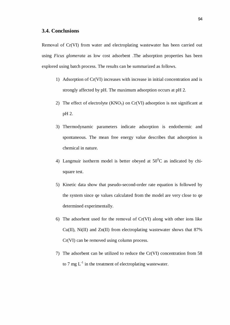
3.3.5 Thermodynamic studies

The temperature range used in this study was 300-500C.The equilibrium

constants (Kc) at 300, 400 and 500C were calculated from the following relation [41]

Kc = CAC/Ce --------------------------------- (8)

Where CAC and Ce are the equilibrium concentrations (mg L-1) of Cr(IV) on the

adsorbent and in solution, respectively. Free energy change (∆G0) can be calculated as

∆G0 = - RT ln Kc --------------------------------- (9)

Where T is the absolute temperature and R is gas constant. The value of

enthalpy change (∆H0) and entropy change (∆S0) were calculated from the following

relation.

ln Kc = (∆S0/R) – (∆H0/R)×(1/T) -------------------------------- (10)

∆S0 and ∆H0 were calculated from the slope and intercept of linear plot of ln Kc

verses 1/T (Fig. 3.9). The values of Kc, ∆H0, ∆S0and ∆G0 are reported in Table 3.3.

The positive value of ∆H0 indicates endothermic process. The decrease in ∆G0 with

increase in temperature indicates that the process is spontaneous and spontaneity

increases with increase in temperature. The positive value of ∆S0 suggests increase

randomness at the solid-liquid interface during adsorption.

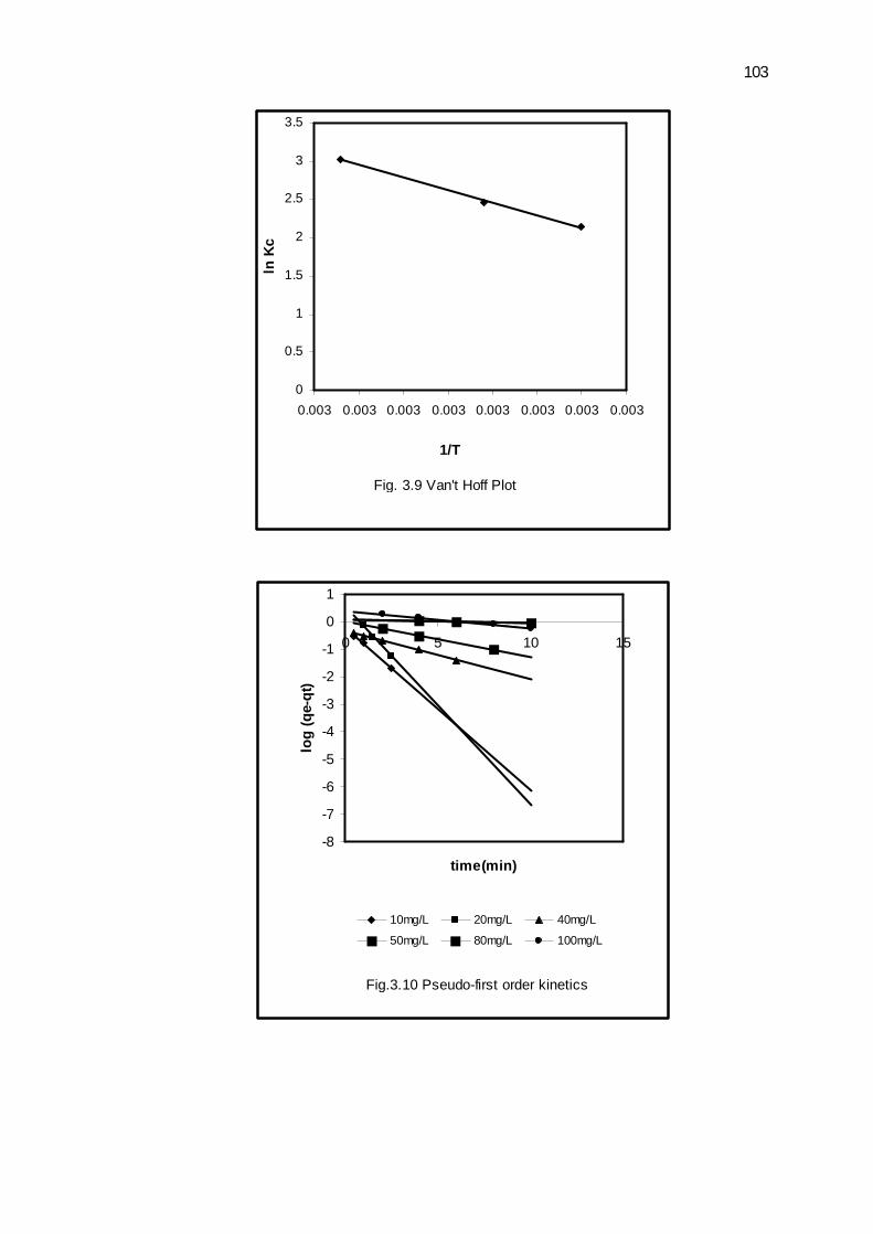
3.3.6 Adsorption kinetics

The rate constants for the adsorption of Cr(VI) were calculated by using

pseudo-first-order & pseudo-second-order equations. The pseudo-first-order [42] and

pseudo-second-order [43] equations are based on solution concentration. The pseudo-

first-order expression is given by equation.

log (qe – qt) = log qe – (K1/2.303)× t ------------------- (11)

92

Where qe is the adsorption capacity (mg g-1) at equilibrium, qt is the adsorption

capacity at time (t) and K1 (min-1) is the pseudo-first-order adsorption rate constant.

Linear plots of log (qe – qt) verses t were observed at different initial Cr(VI)

concentrations (Fig. 3.10). The regression coefficients (R²) and rate constants at

various concentrations are reported in Table 3.4. The pseudo-second-order adsorption

kinetics rate equation [44] is given as

t /qt = 1/h + (1/qe) × t ----------------------------------- (12)

Where h is the initial adsorption rate (mg g-1 min-1), which is given as h = K2 × qe2

K2 (g mg-1 min-1) is the rate constant for pseudo-second-order reaction. The

values of K2 were calculated from the slope of the linear plots of t /qt verses t (Fig.

3.11). These values are reported in Table 3.4. A comparison of the experimental

adsorption capacities (qe(exp)) and calculated values (qe(cal)) obtained from Equation

(11) and (12) show that pseudo-second order model obeyed better than pseudo-second

order.

3.3.7 Intra-particle diffusion:

The Weber and Morris [45] intra-particle diffusion model can be expressed as

qt = Kid × t1/2 + I ----------------------- (13)

Where qt (mg g-1) is the amount of Cr(VI) adsorbed at time t, I (mg g-1) is the

intercept and Kid (mg g-1 min-1/2) is the intra-particle diffusion rate constant. The Kid

values obtained from the slope of the curves at different initial Cr(VI) concentrations

(Fig. 3.12) are shown in Table 3.5. The R2 values (between 0.8842 and 0.9894)

suggest that adsorption of Cr(VI) can be followed by intra-particle diffusion model.

However, plots did not pass through the origin (the intercept values are between 0.20

and 5.1mg g-1) indicating that intra-particle diffusion is not the only rate – limiting

93

step. The increase in intercept values with increase in concentration is indicative of

increased boundary layer effect [46].

3.3.8 Breakthrough capacity

Break through curve is the most effective column process making the

optimum use of the concentration gradient between the solute adsorbed by the

adsorbent and that remaining in the solution. The column is operational until the metal

ions in the effluent start appearing and for practical purposes the working life of the

column is over called breakthrough point. This is important in process design because

it directly affects the feasibility and economics of the process [47]. Fig.3.13 shows

breakthrough curve when a solution containing 50 mg L-1 Cr(VI) passed through the

column packed with 0.5g adsorbent at pH 2. The curve indicates that 50 mL of Cr(VI)

solution can be passed through the column without detecting Cr(VI) in the effluent.

The breakthrough capacity and exhaustive capacities were found to be 5 and 23.1 mg

g-1 respectively.

3.3.9 Treatment of electroplating wastewater

The analysis of electroplating waste water is reported in Table 3.6. On

comparing the analysis of electroplating wastewater before and after treatment it can

be inferred that electroplating wastewater can be treated more efficiently by column

process as concentration of Cr(VI) reduced from 58 to 7 mg L-1 corresponding to

87.93% removal of Cr(VI).

The maximum monolayer adsorption capacity of Ficus for Cr(VI) is compared

with other adsorbents, reported earlier (Table 3.7). The adsorption capacity of Ficus is

comparable or higher than those reported in the literature.

94

3.4. Conclusions

Removal of Cr(VI) from water and electroplating wastewater has been carried out

using Ficus glomerata as low cost adsorbent .The adsorption properties has been

explored using batch process. The results can be summarized as follows.

1) Adsorption of Cr(VI) increases with increase in initial concentration and is

strongly affected by pH. The maximum adsorption occurs at pH 2.

2) The effect of electrolyte (KNO3) on Cr(VI) adsorption is not significant at

pH 2.

3) Thermodynamic parameters indicate adsorption is endothermic and

spontaneous. The mean free energy value describes that adsorption is

chemical in nature.

4) Langmuir isotherm model is better obeyed at 500C as indicated by chi-

square test.

5) Kinetic data show that pseudo-second-order rate equation is followed by

the system since qe values calculated from the model are very close to qe

determined experimentally.

6) The adsorbent used for the removal of Cr(VI) along with other ions like

Cu(II), Ni(II) and Zn(II) from electroplating wastewater shows that 87%

Cr(VI) can be removed using column process.

7) The adsorbent can be utilized to reduce the Cr(VI) concentration from 58

to 7 mg L-1 in the treatment of electroplating wastewater.

95

Table 3.1: Langmuir and Freundlich isotherms parameters for the adsorption of Cr(VI)

Table 3.2: Dubinin-Radushkevisk (D-R) parameters for the adsorption of Cr(VI) at pH 2 Temperature β ln qm qm E R² (ºC) (mol2 kJ ˉ2) (mol g-1) (Kj molˉ¹) x10-5 30 -0.0130 -06.97 93.80 6.2 0.9980 40 -0.0061 -10.25 03.50 9.1 0.9953 50 -0.0062 -09.38 8.37 9.0 1.0000 Table 3.3: Thermodynamic parameters at different temperatures for the adsorption of Cr(VI) at pH 2 Temperature Kc ∆G˚ ∆H˚ ∆S˚ R² (˚C) (kJ mol-1) (kJ mol-1) (kJ mol-1K-1) 30 8.60 -5.40 40 11.82 -6.43 62.74 0.239 0.9978 50 20.70 -8.14

Langmuir isotherm parameters Freundlich isotherm parameters

Temperature (0C)

qm

(mgg-1)

b (Lmg-

1)

R2

χ2

RL

Kf

1/n

R2

χ2

30 40 50

31.60 14.43 46.73

0.0145 0.0502 0.0236

0.9980 0.9914 0.9998

3.490 0.652 0.168

0.5797 0.2849 0.4587

0.0388 1.0900 1.0400

2.097 0.631 0.959

0.9990 0.9991 0.9951

2.07 4.30 0.95

96

Table 3.4: Pseudo-first-order and pseudo-second-order rate parameters for the adsorption of Cr(VI) at different concentrations (pH 2)

Concentration Pseudo-first-order Pseudo-second-order (Co) (mgLˉ¹) qe(exp) qe(cal) K1 R² qe(cal) K2 h R² (mggˉ¹) (mggˉ¹) 10 0.72 0.640 1.37 0.999 0.75 0.93 1.83 0.9944 40 2.70 0.476 0.41 0.997 2.77 2.22 16.20 0.9990 50 3.80 1.047 0.29 0.996 3.90 0.60 8.69 0.9999 80 6.50 1.250 0.34 0.982 6.40 0.16 7.03 0.9984 100 8.10 0.397 0.14 0.995 7.94 0.19 12.80 0.9996 Table 3.5: Intra-particle diffusion parameters for the adsorption of Cr(VI) at pH 2

Table 3.6: Analysis of electroplating wastewater

Parameters Concentration (mgL-1) pH 5.60 TDS 700.00 Na+ 160.00 K+ 2.00 Ca2+ 29.00 Cu2+ 5.60 Cd2+ 1.30 Zn2+ 0.99 Ni2+ 2.00 Cr6+ 58.00

Concentration Kid I R² (mgL-1) (mg g-1 min-1/2) (mg g-1) 10 0.3075 0.2078 0.9612 40 0.2018 2.1865 0.9728 50 0.3471 2.7456 0.9590 80 1.0256 3.0084 0.8842 100 0.7486 5.1853 0.9894

97

Table 3.7: Comparison of the adsorption capacities for Cr(VI) onto various adsorbents Adsorbent adsorption capacity Reference (mg g-1) Spirogyra sp 14.70 [48] Coconut shell based activated carbon 20.00 [49] Palm pressed-fibers 15.00 [50] Almond 10.00 [51] Distillery sludge 5.70 [52] Walnut shell 1.33 [53] Soya cake 0.28 [54] Ficus glomerata 46.73 present study

98

Fig.3.1a SEM image of native adsorbent

Fig.3.1b SEM image of adsorbent after Cr(VI) adsorption

99

Fig.3.2a FTIR of native adsorbent

Fig.3.2b FTIR after Cr(VI) adsorption

100

Fig.3.3 Effect of contact time and initial concentration

0

1

2

3

4

5

6

7

8

0 2 4 6 8 10

time (min)

Adso

rptti

on c

apac

ity (m

g/g)

10 mg/L

20 mg/L

50 mg/L

80 mg/L

100 mg/L

Fig.3.4 Effect of electrolyte cocentration on the adsorption of Cr(VI) at different pH

0

20

40

60

80

100

120

0 2 4 6 8 10 12

pH

% A

dsor

ptio

n

Cr(VI) +DDW

Cr(VI) + 0.01N KNO3

Cr(VI) + 0.1N KNO3

101

Fig.3.5 Point of zero charge

-5

-4

-3

-2

-1

0

1

2

3

0 1 2 3 4 5 6 7 8 9 10

pHi

pHi -

pHf

0.001 N KNO30.01 N KNO30.1N KNO3DDW

Fig. 3.6 Langmuir plots for the adsorption of Cr(VI) on Ficus glomerata

0

0.2

0.4

0.6

0.8

1

1.2

0 0.2 0.4 0.61/Ce

1/qe

30C

40C

50C

102

Fig. 3.7Frendulich plots for the adsorption of Cr(VI) on Ficus glomerata

-0.2

0

0.2

0.4

0.6

0.8

1

1.2

0 0.5 1 1.5

log Ce

log

qe

30C

40C

50C

Fig. 3.8 D.R plots

-18

-16

-14

-12

-10

-8

-6

-4

-2

00 200 400 600 800

ε²

ln q

e

30C

40C

50C

103

Fig. 3.9 Van't Hoff Plot

0

0.5

1

1.5

2

2.5

3

3.5

0.003 0.003 0.003 0.003 0.003 0.003 0.003 0.003

1/T

ln K

c

Fig.3.10 Pseudo-first order kinetics

-8

-7

-6

-5

-4

-3

-2

-1

0

1

0 5 10 15

time(min)

log

(qe-

qt)

10mg/L 20mg/L 40mg/L

50mg/L 80mg/L 100mg/L

104

Fig.3.11 Pseudo-second-order kinetics

0

0.5

1

1.5

2

2.5

3

3.5

0 2 4 6 8 10 12time(min)

qt

10 mg/L 40 mg/L 50 mg/L 80 mg/L 100 mg/L

Fig. 3.12 Intra-particle diffusion

0

1

2

3

4

5

6

7

8

0 0.5 1 1.5 2 2.5 3 3.5

t1/2(min)

qt

10 mg/L 30 mg/L 50 mg/L 80 mg/L 100 mg/L

105

Fig. 3.13 Breakthrough capacity

0

0.05

0.1

0.15

0.2

0.25

0 100 200 300 400

volume of effluent(mL)

C/Co

106

References:

[1] R.S. Prakasham, J.S. Merrie, R.Sheela, N. Saswathi, S.V. Ramakrisha,

Environ pollut.104 (1999) 421-427.

[2] S.M. Nomanbhay, K. Palanisamy.,Electon. J. Biotecnol. 8 (1), (2005)43-53.

[3] C.Raji, T.S. Anirudhan., Water Res.32 (1998) 3772-3780.

[4] F.C.Richard, A.C.M.Bourg., Water Res. 25, (27), (1991) 807-816.

[5] WHO, Guidelines for Drinking Water Quality, vol. 1, 2nd ed., World Health

Organization, (1993).

[6] D. Mohan, K.P. Singh, V.K. Singh., Ind. Eng. Chem. Res.44 ,( 4) ,( 2005)

1027-1042.

[7] G. Tiravanti, D. Ptruzzelli, R. Passino., Water Sci.Technol. 36, (2-3), (1997)

197-207.

[8] C.A. Kozlowski, W. Walkwiak.., Water Res. 36 (2002) 4870-4876.

[9] N. Kongsricharoern, C. Poolprasert., Water Sci. Technol. 34 (1996) 109-1 16.

[10] J.J. Testa, M.A. Grela, M.I. Litter., Environ. Sci. Technol. 38 ,(5), (2002)

1589-1594.

[11] V.K. Gupta, A.K. Shrivastava, N. Jain., Water Res. 35 (2001) 4079- 4085.

[12] Mustafa Yavuz, Fethiye Gode, Erol Pehlivan, Sema Ozmert,

Yogesh.C.Sharma., J.Chem.Eng .137 (2008) 453-461.

[13] P.Goyal, S.Shrivastava. J.Hazard.Mater. 172 (2009) 1206-1211.

[14] Y.S.Sharma, B.Singh, A.Agrawal, C.H.Weng., J.Hazard.Mater. 15 (2008)

789-793.

[15] Parul Sharma, Pushpa Kumari, M.M. Srivastava., Bioresour Technol.98, (2),

(2007) 474-477.

107

[16] P.Goyal, P.Sharma, S.Shrivastava, M.M.Shrivastava., Arch.Environ.Prot.33

(2007) 35-44.

[17] O.D. Uluozlu, A. Sari, M. Tuzen, M. Soylak., Bioresour Technol. (2008)

2972-2980.

[18] J.R. Memon, S.Q. Memon, M.I. Bhanger, A. El-Turki, K.R. Hallam, G.C.

Allen.,Colloids .Surf.B.66 (2009) 232-237.

[19] J. Acharya, J.N. Sahu, B.K. Sahoo, C.R. Mohanty, B.C. Meikap., J.Chem.Eng.

150 (2009) 25-39.

[20] A .El Nemr., J.Hazard. Mater. 161 (2009) 132-141.

[21] M. Jain, V.K. Garg, K. Kadirvelu., J. Hazard. Mater. 162 (2009) 365-372.

[22] H. Gao, Y. Liu, G, Zeng, W. Xu, T. Li, W. Xia.,J.Hazard.Mater.150 (2008)

446-452.

[23] P.Goyal, S.Shrivastava., Arch.Environ. Prot 34 (2008) 35-45.

[24] Chih-Huang Weng, Y.C.Sharma, Sue-Hua Chu., J.Hazard.Mater. 155(2008)

65-75.

[25] C.V. Rao, A.R.Verma, M. V. Kumar, S. Rastogi., J.Ethnopharmacol 115, (2)

(2008) 323-326.

[26] D. H. Lataye, I. M. Mishra, I. D. Mall., Ind. Eng. Chem. Res. 45 (2006) 3934

– 3943.

[27] R. Chand, K. Narimura, H. Kawakita, K. Ohto, T. Watari, K.Inoue., J. Hazard.

Mater. 163 (2009) 245-250.

[28] M. Iqbal, A. Saeed, S. I. Zafar, FTIR spectroscopy., J.Hazard. Mater.

164(2009) 161-171.

[29] S.A. Dean, J.M. Tobin., Resources Conservation and Recycling 27 (1999)

151-156.

108

[30] R.S. Prakasham, J.S. Merrie, R. Sheela, N. Saswathi, S.V. Ramakrisha,

Environ.Pollut 104 (1999) 421-427.

[31] Y. Saga, T. Kutsal., Biotechnol Lett 11 (1989) 141-144.

[32] Xue-Pin Liao, Wei Tang, Rong-Qing Zhou, Bi Shi., Adsorption.14 (2008) 55-

64.

[33] A.Baran, E, Bicak, S.H. Baysal, S. Onal., Bioresour.Technol. 98 (2007) 661-

665.

[34] H. Ucun, Y.K. Bayhan, Y. Kaya, A. Cakici, O.F. Algm., Bioresour. Technol.

85 (2002) 155-158.

[35] B.M. Babic, S.K. MLonjie, M.J. Polovina, B.V. Kaludierovic., Carbon 37

(1999) 477- 481.

[36] M. Ajmal, R.A. K. Rao, R. Ahmad, J. Ahmad., J.Hazard. Mater. B 87 (2001)

127-137

[37] Y.S. Ho.,Carbon 42 (2004) 2113-2130.

[38] L. Ghodbane, O.Nouri, M.Hamdaoui, Chiha. J.hazard. Mater. 152 (2008) 148-

158.

[39] M. M. Dubinin and L.V. Radushkevich, Proc. Acad. Sci. USSR, Phys. Chem.

Sect. 55 (1947) 331.

[40] F.Helfferich, Ion-exchange. Mc Graw. Hill, New York, 1962.

[41] C. Namasivayam, K. Ranganatham., Water Res. 29 (1995) 1737-1744.

[42] D. J. O. Shannessy, D. J. Winzor, Anal. Biochem. 236, (2), (1996) 275-283.

[43] Y.S. Ho, G. Mckay., Water Res. 34 (2000) 735-742.

[44] Y.S.Ho, C.C.Wang., Process.Biochem 39, (6), (2004) 761-765.

[45] W.J. Weber Jr, J.C. Morris., J. Sanitary Eng. Div. 89 (1963) 31-59.

[46] Ghodhana, Q. Hamdaoui., J. Hazard. Mater. 160 (2008) 301-309.

109

[47] B. Volesky., BV. Sorbex. Inc. Montreal, Canada. (2003) 183-185.

[48] V.K. Gupta, A.K. Shrivastava, N. Jain., Water Res.35 (2001) 4079-4085.

[49] G.J. Alaerts, V. Jitjaturant, P. Kelderman., Water Sci. and Technol. 21(1989)

1701-1704.

[50] W.T. Tan, S.T. Ooi, C.K. Lee., Environ. Technol. 14 (1993) 227-282.

[51] M. Dakiky, M. Khamis, A. Manassra, M. Mer’eb., Adv. in Environ. Res. 6

(2002) 533-540.

[52] K. Selvaraj, S. Manonmani, S. Pattabhi., Bioresour. Technol. 89 (2003) 207-

211.

[53] Y. Orhan, H. Buyukgungur., Water Sci. and Tecnol. 28(1993) 247-255.

[54] N. Deneshver, D. Salari, S. Aber., J.Hazard. Mater. B 94 (2002) 49-61.