Chapter 21 FIRMS’ DEMANDS FOR INPUTS Copyright ©2002 by South-Western, a division of Thomson...

Chapter 21

FIRMS’ DEMANDS FOR INPUTS

Copyright ©2002 by South-Western, a division of Thomson Learning. All rights reserved.

MICROECONOMIC THEORYBASIC PRINCIPLES AND EXTENSIONS

EIGHTH EDITION

WALTER NICHOLSON

Profit Maximization and Derived Demand

• A firm’s hiring of inputs is directly related to its desire to maximize profits– any firm’s profits can be expressed as the

difference between total revenue and total costs, each of which can be regarded as functions of the inputs used

= TR(K,L) - TC(K,L)

Profit Maximization and Derived Demand

• First-order conditions for a maximum are

0

K

TC

K

TR

K

0

L

TC

L

TR

L

– the firm should hire each input up to the point at which the extra revenue yielded from one more unit is equal to the extra cost

Marginal Revenue Product

• The marginal revenue product (MRP) from hiring an extra unit of any input is the extra revenue yielded by selling what that extra input produces

MRP = MR MP

Marginal Expense

• If the supply curve facing the firm for the inputs it hires are infinitely elastic at prevailing prices, the marginal expense of hiring a worker is simply this market wage

• If input supply is not infinitely elastic, a firm’s hiring decision may have an effect on input prices

Marginal Expense

• For now, we will assume that the firm is a price taker for the inputs it buys

TC/K = v

TC/L = w

• The first-order conditions for profit-maximization become

MRPK = v

MRPL = w

An Alternative Derivation

• The Lagrangian expression associated with a firm’s cost-minimization problem is

L = vK + wL + [q0 - f(K,L)]

• First-order conditions are

L/K = v - (f /K) = 0

L/L = w - (f /L) = 0

L/ = q0 - f (K,L) = 0


• The first two equations can be written as

vMPK

fK

wMPL

fL


• Since can be interpreted as marginal cost in this problem, we have

MC MPK = v

MC MPL = w

• Profit maximization requires that MR = MC so we have

MR MPK = MRPK = v

MR MPL = MRPL = w

Price Taking in theOutput Market

• If a firm exhibits price-taking behavior in its output market, MR = P

• This means that at the profit-maximizing levels of each input

P MPK = v

P MPL = w

– sometimes P multiplied by an input’s MP is called the value of marginal product

Comparative Statics ofInput Demand

• We will focus on the comparative statics of the demand for labor– the analysis for capital would be symmetric

• For the most part, we will assume price-taking behavior for the firm in its output market

Single-Input Case• It is likely that L/w < 0

– this is based on the presumption that the marginal physical product of labor declines as the quantity of labor employed rises

• a fall in w must be met by a fall in MPL for the firm to continue maximizing profits (because P is fixed)

– this argument is strictly correct for the case of one input

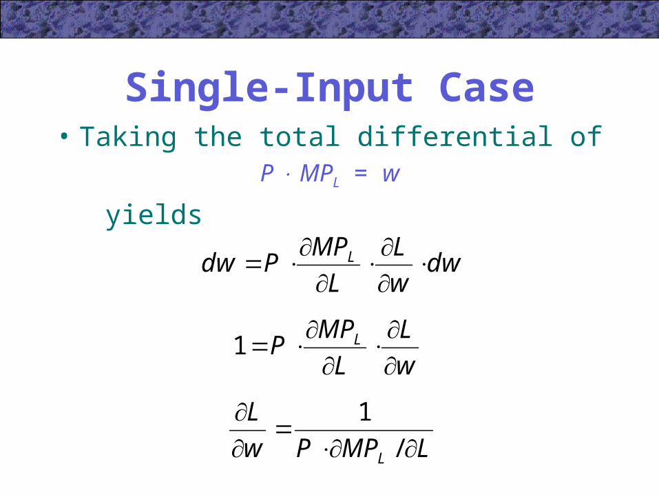
Single-Input Case• Taking the total differential of

P MPL = w

yieldsdw

w

L

L

MPPdw L

w

L

L

MPP L

1

LMPPw

L

L

/

1

Single-Input Case

• If we assume that MPL /L < 0 (MPL falls as L increases), we have

L/w < 0

• A fall in w will cause more labor to be hired– more output will be produced as well

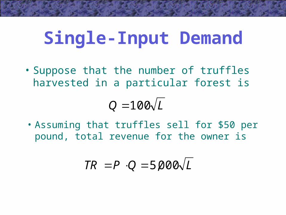
Single-Input Demand

• Suppose that the number of truffles harvested in a particular forest is

LQ 100

• Assuming that truffles sell for $50 per pound, total revenue for the owner is

LQPTR 000,5

Single-Input Demand

• Marginal revenue product is given by

2/1500,2

L

L

TR

• If truffle searchers’ wages are $500, the owner will determine the optimal amount of L to hire by

2/1500,2500 L

25L

Two-Input Case

• If w falls, both L and K will change as a new cost-minimizing combination of inputs is chosen

• When K changes, the entire MPL function changes– labor has a different amount of capital to

work with

• However, we still expect that L /w < 0

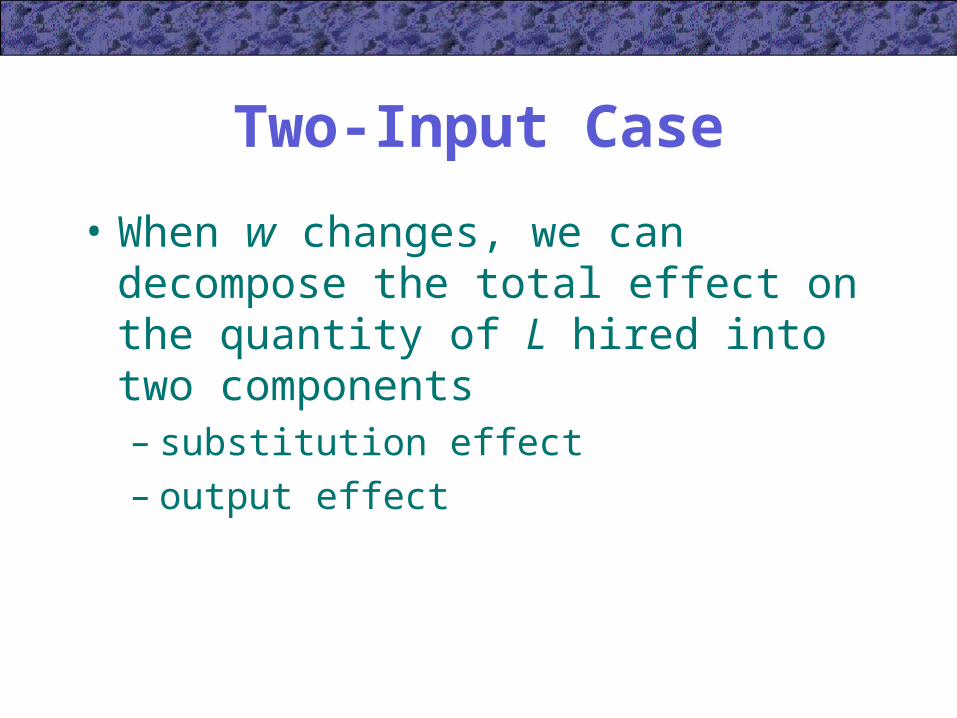
Two-Input Case

• When w changes, we can decompose the total effect on the quantity of L hired into two components– substitution effect– output effect

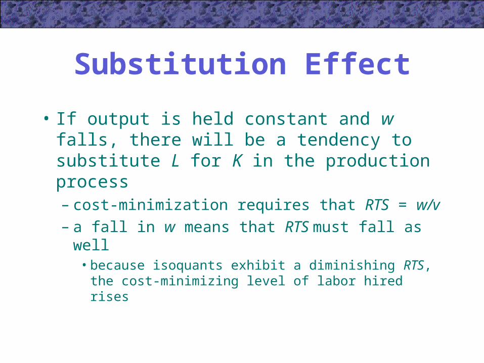
Substitution Effect

• If output is held constant and w falls, there will be a tendency to substitute L for K in the production process– cost-minimization requires that RTS = w/v– a fall in w means that RTS must fall as well

• because isoquants exhibit a diminishing RTS, the cost-minimizing level of labor hired rises

Substitution Effect

L

K

q0

A

The substitution effect is shown holding output constant at q0

K1

L1

v

w1 slope

B

As w falls, the firm will substitute L for K in the production process

K2

L2

v

w2 slope

Output Effect

• A change in w will shift the firm’s expansion path

• This means that the firm’s cost curves will also shift– a drop in w will lower MC and lead to a

higher level of output

• This increase in output will lead to a higher level of L being demanded

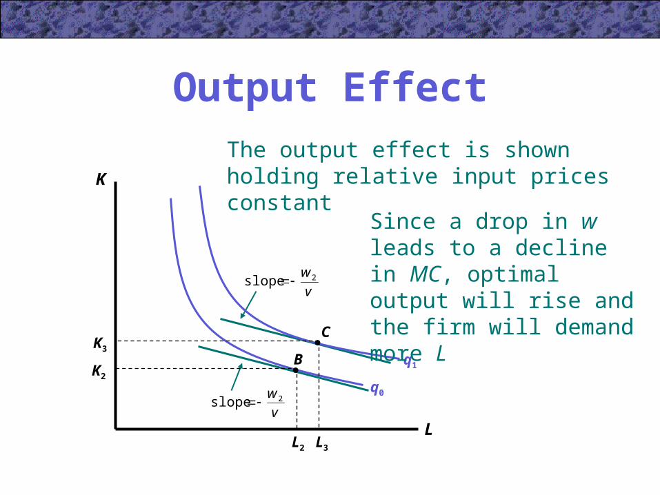
The output effect is shown holding relative input prices constant

v

w2 slope

v

w2 slope

Output Effect

L

K

q0

B

K2

L2

q1

CK3

L3

Since a drop in w leads to a decline in MC, optimal output will rise and the firm will demand more L

Substitution andOutput Effects

L

K

q0

A

K1

L1

B

K2

L2

q1

Both the substitution effect and the output effect lead to a rise in the quantity of L demanded when w falls

CK3

L3

Cross-Price Effects

• No definite statement can be made about how capital will change when w changes

• The substitution and output effects move in opposite directions– a fall in w will lead the firm to substitute

away from K– a fall in w will lead the firm to increase output

and thus demand more K

Mathematical Derivation

• General input demand functions generated by the firm’s profit-maximizing decision are

L = L(P,w,v)

K = K(P,w,v)

• The presence of P in these functions indicates the close connection between product demand and input demand

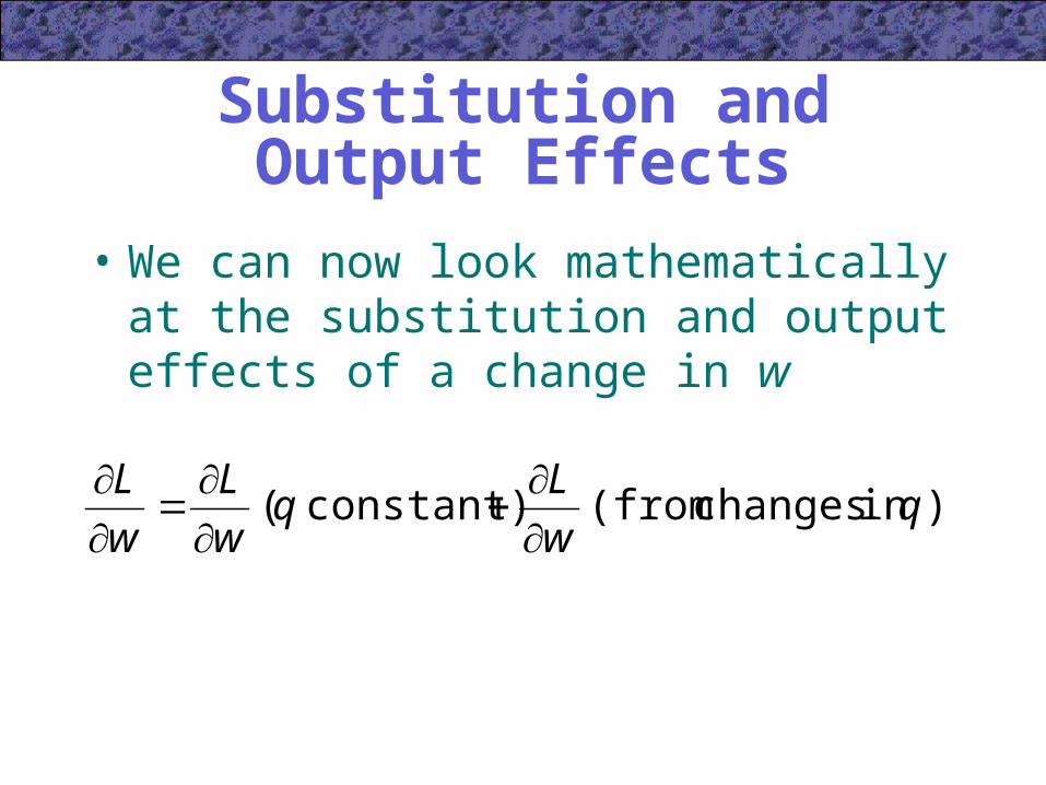
Substitution andOutput Effects

• We can now look mathematically at the substitution and output effects of a change in w

) in changes (from constant) ( qw

Lq

w

L

w

L

Constant OutputDemand Functions

• Shephard’s lemma uses the envelope theorem to show that the constant output demand function for L can be found by partially differentiating total cost with respect to w

),,(' vwqLw

TC

Constant OutputDemand Functions

• Two arguments suggest why L’/w < 0– in the two-input case, the assumption of a

diminishing RTS combined with the assumption of cost-minimization requires that w and L move in opposite directions when output is held constant

– even in the many-input case, L’/w = 2TC/w2 < 0 if costs are truly minimized

Output Effects

• We can use a “chain rule” argument to examine the causal links that determine how changes in w affect the demand for L through induced output changes

w

MC

MC

P

P

q

q

Lq

w

L

) in changes (from

Output Effects

P/MC = 1 because P=MC for profit maximization under perfect competition

q/P < 0 since there is an inverse relationship between the firm’s price and its share of market demand

L/q and MC/w must have the same sign

w

MC

MC

P

P

q

q

Lq

w

L

) in changes (from

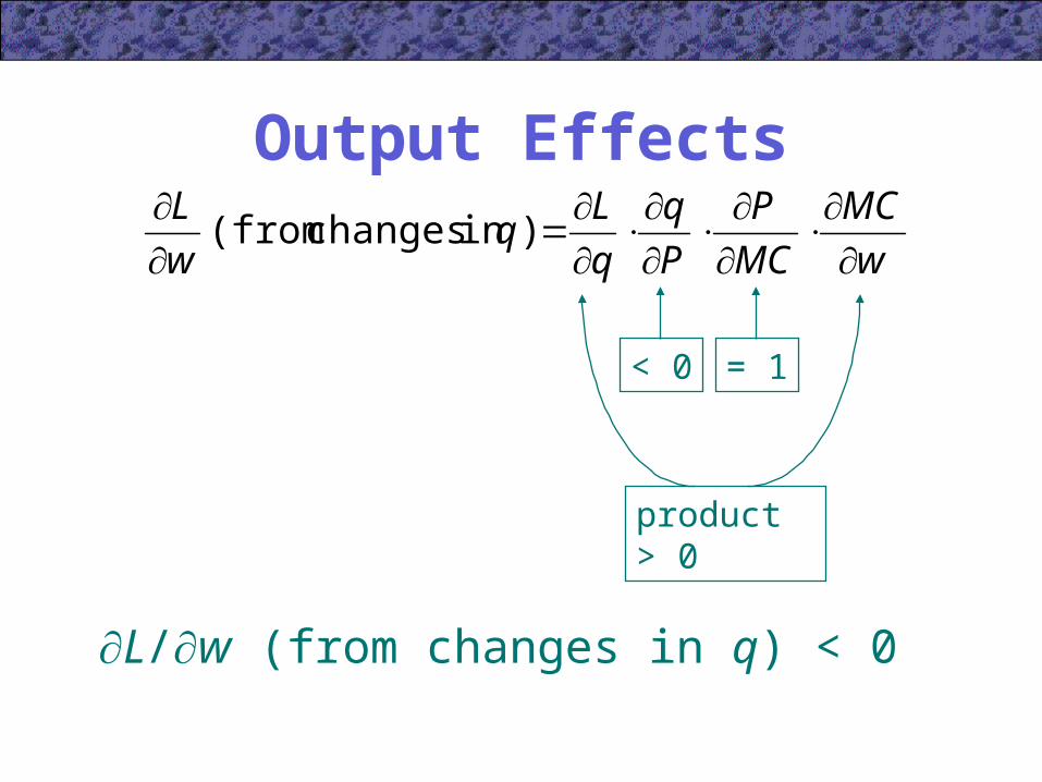
Output Effects

w

MC

MC

P

P

q

q

Lq

w

L

) in changes (from

< 0 = 1

product > 0

L/w (from changes in q) < 0

Mathematical Derivation

• The mathematical conclusion is that L/w < 0– substitution and output effects move in the

same direction

Decomposing Input Demand

• The short-run supply function for a hamburger producer is

5.0)(

)10(40

vw

Pq

• The firm’s demand for labor is

5.15.0

2)10(

wv

PL


• If w = v = $4 and P = $1, the firm will produce 100 hamburgers hire 6.25 workers

• If w rises to $9 while v and P remain unchanged, the firm will produce 66.6 hamburgers and hire only 1.9 workers


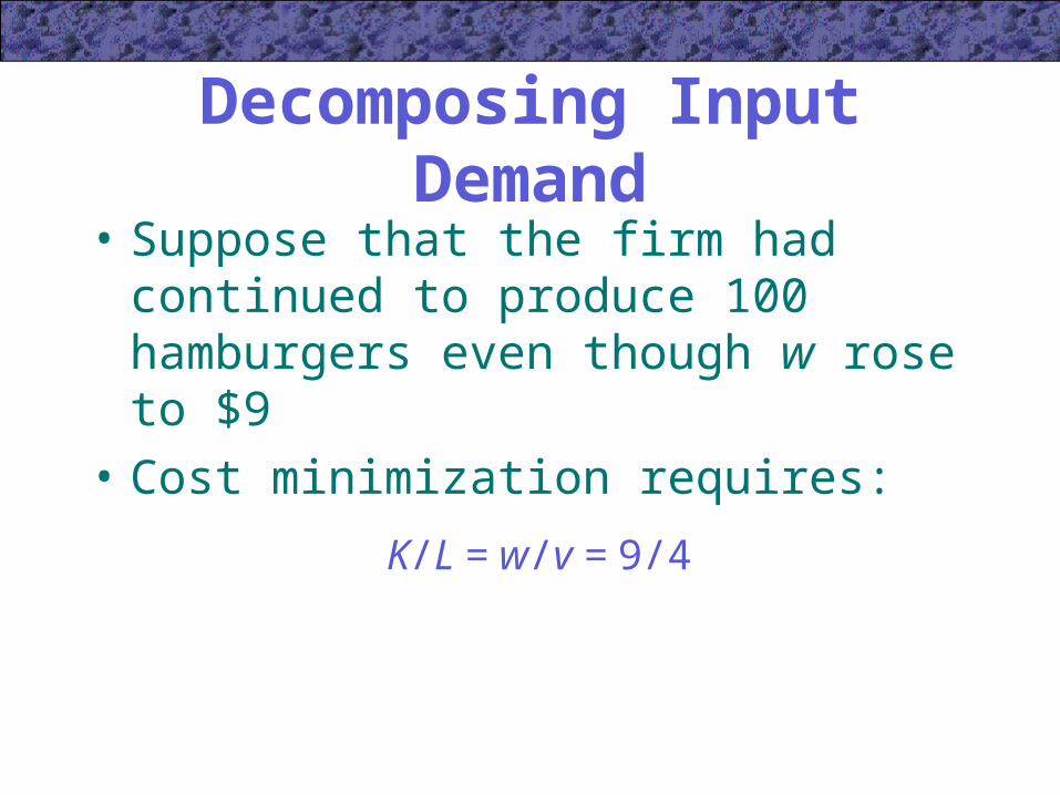
• Suppose that the firm had continued to produce 100 hamburgers even though w rose to $9

• Cost minimization requires:

K/L = w/v = 9/4

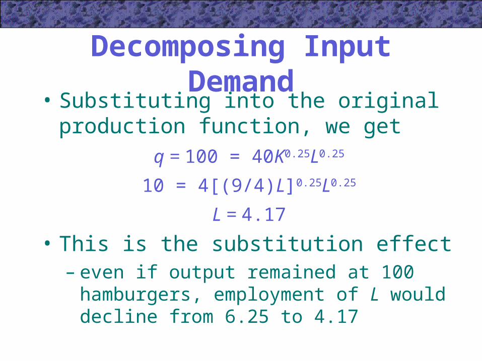
Decomposing Input Demand• Substituting into the original production

function, we get

q = 100 = 40K0.25L0.25

10 = 4[(9/4)L]0.25L0.25

L = 4.17

• This is the substitution effect– even if output remained at 100 hamburgers,

employment of L would decline from 6.25 to 4.17

Decomposing Input Demand• We can compute the constant output

demand for labor using Shephard’s lemma

• Total costs are

TC = vK + wL

• If we substitute the input demand functions, we get

TC = [q2v0.5w0.5]/800

Decomposing Input Demand• Applying Shephard’s lemma yields

600,1'

5.05.02

wvq

w

TCL

• For q = 100, we have

L’ = 6.25v0.5w -0.5

• If v = w = $4, L’ = 6.25

• If w changes to $9, L’ = 4.17


• Note how the constant output demand function (L’) allows us to hold output constant in our analysis, while the total demand function (L) allows output to change– there will be a larger impact of a wage

change when using the total demand function

Responsiveness of Input Demand to Changes

in Input Prices• We can now explain the degree to

which input demand will respond to changes in input prices

• When w rises, will the decline in L be large or small?


in Input Prices• Substitution effect

– this will depend on how easy it is to substitute other inputs for L

• the elasticity of substitution for the firm’s production function

• the length of time allowed for adjustment


in Input Prices• Output effect

– this will depend on the size of the decline in output

• how important labor is in the firm’s total costs• the price elasticity of demand for the output


in Input Prices• The price elasticity of demand for any

input will be greater (in absolute value),– the larger is the elasticity of substitution for

other inputs– the larger is the share of total cost

represented by expenditures on that input– the larger is the price elasticity of demand for

the good being produced

Elasticity of Demand for Inputs

• Suppose that the constant output demand for labor for our hamburger producer is

L’ = (q2v0.5w -0.5)/1,600

• The constant output wage elasticity of demand (LL) is

5.0ln

'ln

w

L

L'

w

w

L'LL


• Suppose that labor costs represent half of all variable costs– sL = 0.5

• This implies that

LL = sL – 1 = -(1 – sL) = -0.5

• This result is a special case of

LL = -(1 – sL)

Elasticity of Demand for Inputs• In order to quantify output effects, we will

need to use an elasticity form of the chain of events that occurs when the wage changes

eL,w (from changes in q) = eL,q eq,P eP,MC eMC,w

• If P is assumed constant and MC is a linear function of q, any increase in P must result in a proportional change in q

– this implies that eq,P eP,MC = -1


• In addition, we know that

– using the TC curve shown earlier, we can calculate eMC,w = 0.5

– because the production function exhibits diminishing returns to scale, eL,q = 1/eq,L = 2 for movements along the expansion path


• Thus,

eL,w (from changes in q) = (2)(-1)(0.5) = -1

and the total elasticity of demand (including substitution and output effects) is

eL,w = -0.5 – 1.0 = -1.5

Elasticity of Demand for Inputs• When the change in w affects all firms,

the price of the product will change– In the long run, with constant returns to

scale, eL,q = 1, eP,MC = 1, and eMC,w = sL

• The output effect can be written aseL,w (from changes in q) = sLeq,P

• The total wage elasticity iseL,w = LL + sLeq,P = -(1 – sL) + sLeq,P

Competitive Determination of Income Shares

• Assume there is only one firm producing a homogeneous output using L and K

• The production function for the firm is Q = f(K,L) and output sells at a price of P

• The total income received by labor is wL, while the total income accruing to capital is vK

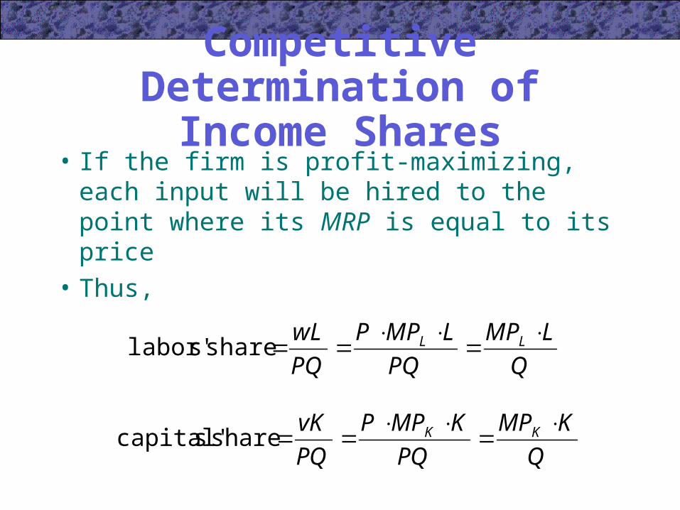
Competitive Determination of Income Shares

• If the firm is profit-maximizing, each input will be hired to the point where its MRP is equal to its price

• Thus,

Q

LMP

PQ

LMPP

PQ

wL LL

share slabor'

Q

KMP

PQ

KMPP

PQ

vK KK

share scapital'

Factor Shares and the Elasticity of Substitution

• The elasticity of substitution is defined as

)/(%

)/(%

vw

LK

– If = 1, the relative shares of K and L will remain constant as the capital-labor ratio rises

– If > 1, the relative share of K will rise as the capital-labor ratio increases

– If < 1, the relative share of K will fall as the capital-labor ratio increases

Monopsony in theLabor Market

• In many situations, the supply curve for an input (L) is not perfectly elastic

• We will examine the polar case of monopsony, where the firm is the single buyer of the input in question– the firm faces the entire market supply curve– to increase its hiring of labor, the firm must

pay a higher wage


• The marginal expense of hiring an extra unit of labor (MEL) exceeds the wage

• If the total cost of labor is wL, then

L

wLw

L

wLMEL

• In the competitive case, w/L = 0 and MEL = w

• If w/L > 0, MEL > w


Labor

Wage

S

ME

D

L1

The firm will set MEL = MRPL to determine its profit-maximizing level of labor (L1)

w1

The wage is determined by the supply curve


Labor

Wage

S

ME

D

L1

w1

Note that the quantity of labor demanded by this firm falls short of the level that would be hired in a competitive labor market (L*)

L*

w* The wage paid by the firm will also be lower than the competitive level (w*)

Monopsonistic Hiring

• Suppose that a coal mine’s workers can dig 2 tons per hour and coal sells for $10 per ton– this implies that MRPL = $20 per hour

• If the coal mine is the only hirer of miners in the local area, it faces a labor supply curve of the form

L = 50w

Monopsonistic Hiring

• The firm’s wage bill iswL = L2/50

• The marginal expense associated with hiring miners is

MEL = wL/L = L/25

• Setting MEL = MRPL, we find that the optimal quantity of labor is 500 and the optimal wage is $10

Monopoly in theSupply of Inputs

• Imperfect competition may also occur in input markets if suppliers are able to form a monopoly– labor unions in “closed shop” industries– production cartels for certain types of

capital equipment– firms (or countries) that control unique

supplies of natural resources


• If both the supply and demand sides of an input market are monopolized, the market outcome will be indeterminate– the actual outcome will depend on the

bargaining skills of the parties


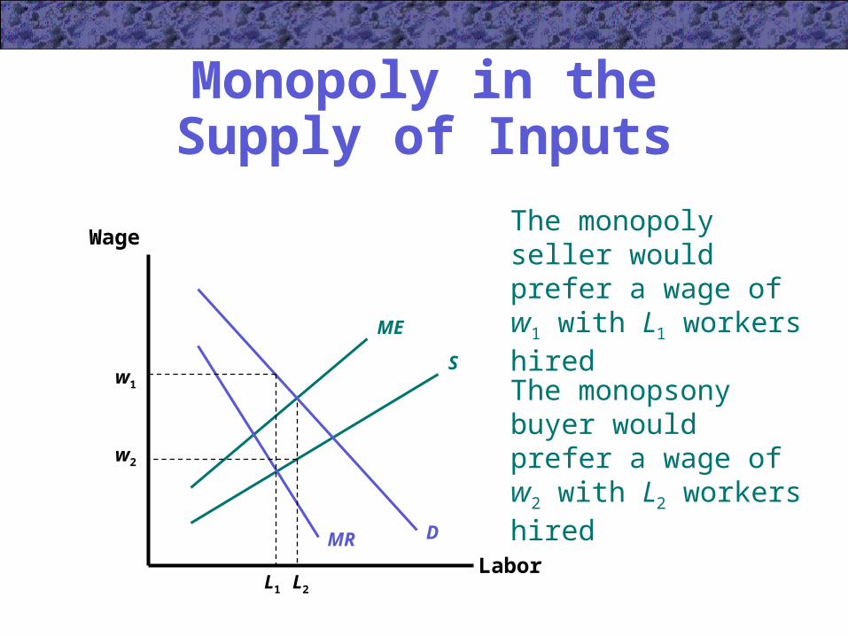
Labor

Wage

S

ME

DMR

L1

w1

The monopoly seller would prefer a wage of w1 with L1 workers hired

L2

w2

The monopsony buyer would prefer a wage of w2 with L2 workers hired

Important Points to Note:

• The marginal revenue product from hiring extra units of an input is the combined influence of the marginal physical product of the input and the firm’s marginal revenue in its output market


• If the firm is a price taker for the inputs it buys, it is possible to analyze the comparative statics of its demand fairly completely– a rise in the price of an input will cause

fewer units to be hired because of substitution and output effects

• the size of these effects will depend on the firm’s technology and on the price responsiveness of the demand for its output


• The marginal productivity theory of input demand can also be used to study the determinants of relative income shares accruing to various factors of production– the elasticity of substitution indicates how

these shares change in response to changing factor supplies


• If a firm has a monopsonistic position in an input market, it will recognize how its hiring affects input prices– the marginal expense associated with hiring

additional units of an input will exceed that input’s price, and the firm will reduce hiring below competitive levels to maximize profits


• If input suppliers form a monopoly against a monopsonistic demander, the result is indeterminate– in such a situation of bilateral monopoly, the

market equilibrium chosen will depend on the bargaining of the two parties

Chapter 21 FIRMS’ DEMANDS FOR INPUTS Copyright ©2002 by South-Western, a division of Thomson...

Documents

Transcript of Chapter 21 FIRMS’ DEMANDS FOR INPUTS Copyright ©2002 by South-Western, a division of Thomson...