Chapter 2. Unobserved Component models

Esther Ruiz2006-2007

PhD Program in Business Administration and Quantitative Analysis

Financial Econometrics

2.1 Description and propertiesUnobserved component models assume that the

variables of interest are made of components with a direct interpretation that cannot be directly observed

Applications in finance:“Fads” model of Potterba and Summers (1998).

There are two types of traders: informed (μt) and uninformed (εt). The observed price is yt

ttt

ttty

1

Models for Ex ante interest differentials proposed by Cavaglia (1992): We observe the ex post interest differential which is equal to the ex ante interest differential plus the cross-country differential in inflation

ttt

ttt

yLy

yy

**

*

)( 1

Factor models simplify the computation of the covariance matrix in mean-variance portfolio allocation and are central in two asset pricing theories: CAPM and APT

Nk

rErffE

f

f

f

v

v

v

r

r

r

tttttttt

Nt

t

t

kt

t

t

Nkt

kt

kt

tN

t

t

Nt

t

t

Nt

t

t

11

2

1

2

1

2

1

1

21

11

2

1

2

1

|,|

.........

...

...

...

...

.........

''

Term structure of interest rates model proposed by Rossi (2004): The observed yields are given by the theoretical rates implied by a no arbitrage condition plus a stochastic disturbance

tttttt

nt

t

t

uCrBA

y

y

y

)(

...

)(

)(

2

1

tt

u

t

t

t cu

r

tbba

tatbta

u

r

exp~

~expexp~exp

01

1

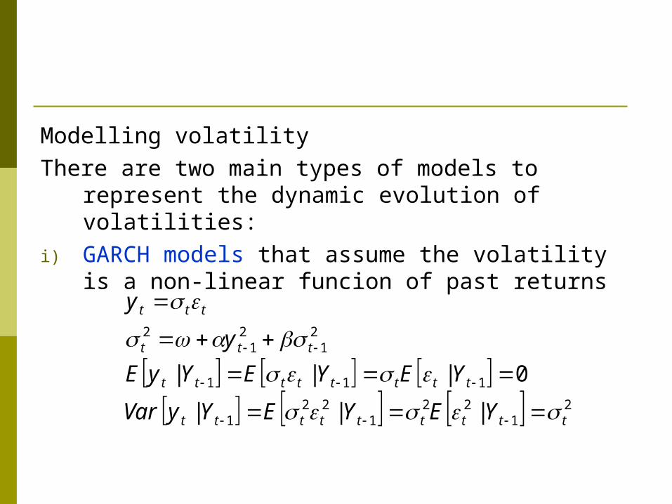
Modelling volatility

There are two main types of models to represent the dynamic evolution of volatilities:

i) GARCH models that assume the volatility is a non-linear funcion of past returns

2

122

122

1

111

21

21

2

0

ttttttttt

tttttttt

ttt

ttt

YEYEYyVar

YEYEYyE

y

y

|||

|||

σ is the one-step ahead (conditional) variance and, therefore, can be observed given observations up to time t-1.

As a result, classical inference procedures can be implemented.

Example: Consider the following GARCH(1,1) model for the IBEX35 returns

The returns corresponding to the first two days in the sample are: 0.21and -0.38

21

21

2 889010300190 ttt y ...

951

142889038010300190380210

0380210

142382889021010300190210

0210

2213

213

212

12

.

.*..*..).,.|(

).,.|(

..*..*..).|(

).|(

yyyVar

yyyE

yyVar

yyE

In this case, there are not unobserved components but consider the model for fundamental prices with GARCH errors

In this case, the variances of the noises cannot be observed with information available at time t-1

ttt

ttty

1

2110

2110

ttttt

ttttt

qq

hh

,

,

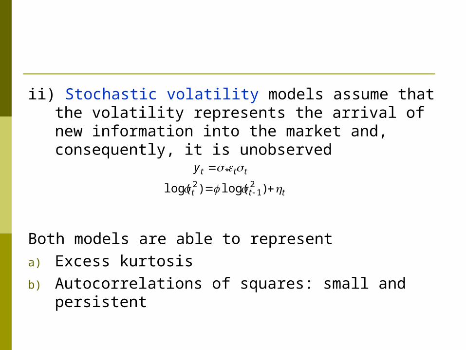
ii) Stochastic volatility models assume that the volatility represents the arrival of new information into the market and, consequently, it is unobserved

Both models are able to represent

a) Excess kurtosis

b) Autocorrelations of squares: small and persistent

ttty *

ttt )log()log( 21

2

Although the properties of SV models are more attractive and closer to the empirical properties observed in real financial returns, their estimation is more complicated because the volatility, σt, cannot be observed one-step-ahead.

2.2 State space modelsThe Kalman filter allows the estimation of the underlying

unobserved components.

To implement the Kalman filter we are writting the unobserved model of interest in a general form known as “state space model”.

The state space model is given by

where the matrices Zt, Ht, Tt and Qt can evolve over time as far as they are known at time t-1.

),(,

),(,

tttttt

tttttt

QNT

HNZy

0

0

1

Consider, for example, the random walk plus noise model proposed to represent fundamental prices in the market.

In this case, the measurement equation is given by

Therefore, Zt=1, the state αt is the underlying level μt and Ht=

The transition equation is given by

and Tt=1 and Qt=

ttttttt yZy

ttttttt T 11

2

2

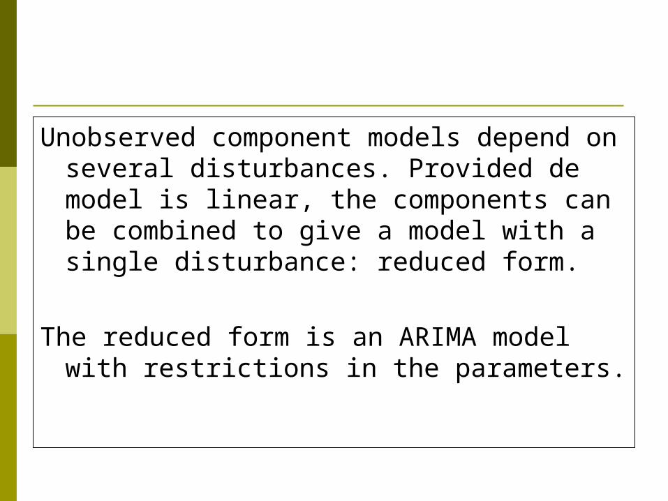
Unobserved component models depend on several disturbances. Provided de model is linear, the components can be combined to give a model with a single disturbance: reduced form.

The reduced form is an ARIMA model with restrictions in the parameters.

Consider the random walk plus noise model

In this case

The mean and variance of are given by

ttt

ttty

1

ttty

ty

0)()( ttt EyE

222 2)()( ttt EyVar

The autocorrelation function is given by

signal to noise ratio.The reduced form is an IMA(1,1) model with

negative parameter where

2,0

1,2

1

2)(

22

2

h

hq

h

2

2

q

2

242 qqq

When, q=0, reduces to a non-invertible MA(1) model, i.e. yt is a white noise process. On the other hand, as q increases, the autocorrelations of order one, and consequently, θ , decreases. In the limit, if , is a white noise and yt is a random walk.

ty

02 ty

Although we are focusing on univariate series, the results are valid for multivariate systems. The Kalman filter is made up of two sets of equations:

i) Prediction equations: one-step ahead predictions of the states and their corresponding variances

For example, in the random walk plus noise model:

111 tttttt aTYEa |/

11 ttt mm /

tttttttttt QTPTYaEP '

// | 1111

211 ttt PP /

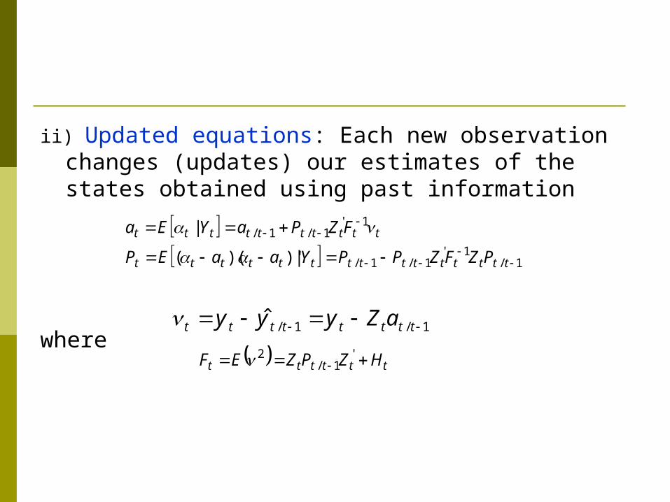
ii) Updated equations: Each new observation changes (updates) our estimates of the states obtained using past information

where

1

111

111

ttttttttttttttt

tttttttttt

PZFZPPYaaEP

FZPaYEa

/'

//

'//

|)')((

|

11 tttttttt aZyyy //ˆ

tttttt HZPZEF '

/ 12

The updating equations can be derived using the properties of the multivariate normal distribution.

Consider the distribution of αt and yt conditional on past information up to and including time t-1.

The conditional mean and variance are: ttttttt caTYEa 111/ |

tttttttt daZYyEy 1/11/ |ˆ

The conditional covariance can be easily derived by writting

tttttttttt aZdaZy )( 1/1/

'

1/

'1/1/

11/1/

11 )))')(((()')(()|,(

ttt

ttttttttt

ttttttttt

ttt

ZP

ZaaEdaZyaEYyCov

tttt

ttttt

tttt

ttt

t

t

FPZ

ZPP

daZ

aNY

y 1/

'1/1/

1/

1/1 ,|

Consider, once more the random walk plus noise model. In this case,

21

11

11

1

1

ttt

t

ttttt

tttt

ttttt

Pf

fP

PP

myf

Pmm

/

//

//

/ )(

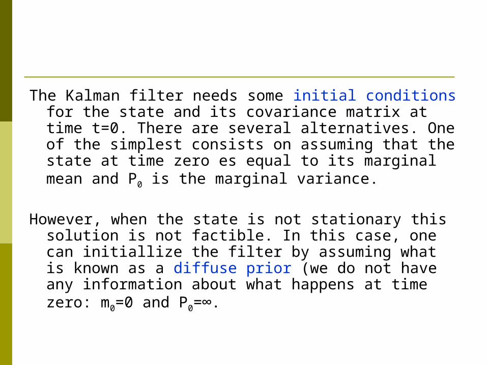
The Kalman filter needs some initial conditions for the state and its covariance matrix at time t=0. There are several alternatives. One of the simplest consists on assuming that the state at time zero es equal to its marginal mean and P0 is the marginal variance.

However, when the state is not stationary this solution is not factible. In this case, one can initiallize the filter by assuming what is known as a diffuse prior (we do not have any information about what happens at time zero: m0=0 and P0=∞.

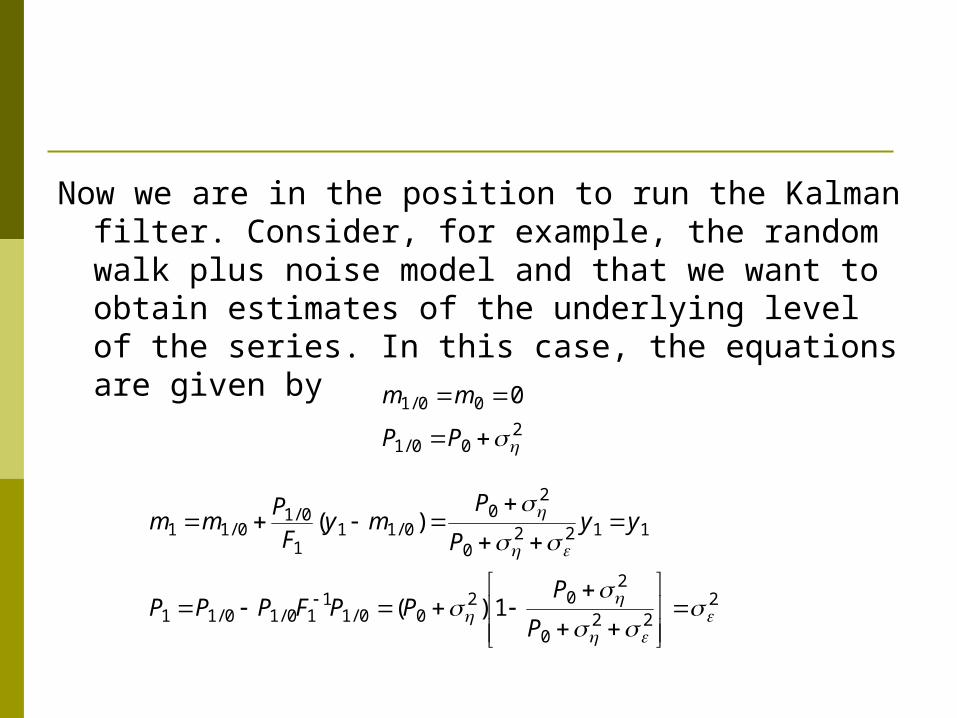
Now we are in the position to run the Kalman filter. Consider, for example, the random walk plus noise model and that we want to obtain estimates of the underlying level of the series. In this case, the equations are given by

2001

001 0

PP

mm

/

/

222

0

202

0011

101011

11220

20

0111

01011

1

P

PPPFPPP

yyP

Pmy

FP

mm

)(

)(

///

//

/

2122

2112

112

/

/

/

Pf

PP

mm

22

1

212

1121

212122

1222

12122

1

P

PPPFPPP

myFP

mm

)(

)(

///

//

/

Consider, for example, that we have observations of a time series generated by a random walk with and

1.14, 0.59, 1.58,….

12 42

8305615

68014159065

141

615

541

141

1

141

2

2

2

12

12

1

1

.)/(

.)..(.

.

.

/

/

P

m

f

P

m

P

m

-30

-20

-10

0

10

20

30

250 500 750 1000

Y PREDICTIONS

-30

-20

-10

0

10

20

250 500 750 1000

PREDICTIONS FILTERED

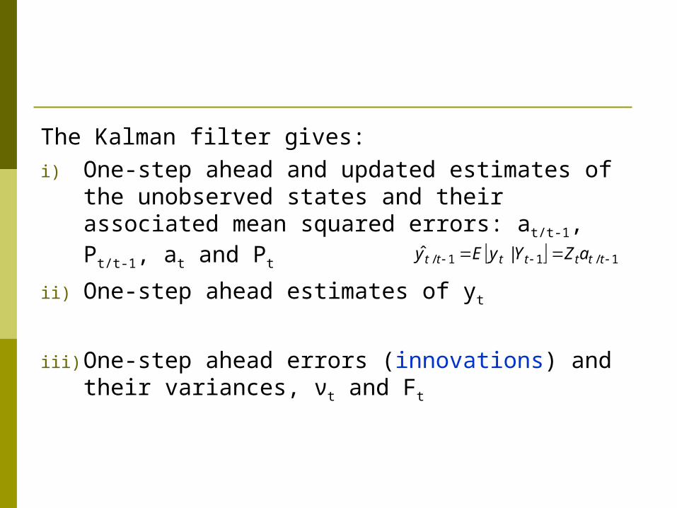
The Kalman filter gives:

i) One-step ahead and updated estimates of the unobserved states and their associated mean squared errors: at/t-1, Pt/t-1, at and Pt

ii) One-step ahead estimates of yt

iii) One-step ahead errors (innovations) and their variances, νt and Ft

111 ttttttt aZYyEy // |ˆ

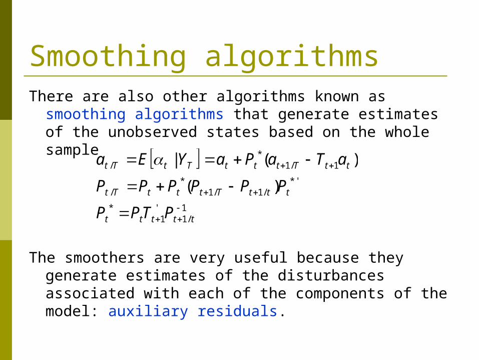
Smoothing algorithmsThere are also other algorithms known as smoothing

algorithms that generate estimates of the unobserved states based on the whole sample

The smoothers are very useful because they generate estimates of the disturbances associated with each of the components of the model: auxiliary residuals.

111

11

11

ttttt

tttTtttTt

ttTtttTtTt

PTPP

PPPPPP

aTaPaYEa

/'*

*'//

*/

/*

/

)(

)(|

For example, in the random walk plus noise model:

)(

)(

//

/

//

/

2121

222

11

111

TTTTT

TTTT

TTTTT

TTTT

aaPP

aa

aaPP

aa

-30

-20

-10

0

10

20

250 500 750 1000

FILTERED SMOOTHED

-30

-20

-10

0

10

20

30

250 500 750 1000

Y SMOOTHED

The auxiliary residuals are useful to:

i) identify outliers in different components; Harvey and Koopman (1992)

ii) test whether the components are heteroscedastic; Broto and Ruiz (2005a,b)

This test is based on looking at the differences between the autocorrelations of squares and the squared autocorrelations of each of the auxiliary residuals; Maravall (1983).

PredictionOne of the main objectives when dealing with time series

analysis is the prediction of future values of the series of interest. This can easily be done in the context of state space models by running the prediction equations without the updating equations:

In the context of the random walk plus noise model:

ZTQTZZTPTZYaaEP

aTZYEa

k

j

jt

jkT

ktkTkTkTkTkT

Tk

tTkTkT

1

0

''

'

''|)')((

|

21 kPP

mm

TTT

TTkT

/

/

Estimation of the parametersUp to now, we have assumed that the parameters of the

state space model are known. However, in practice, we need to estimate them. In Gaussian state space models, the estimation can be done by Maximum Likelihood. In this case, we can write

The expression of the log-likelihood is then given by

T

t

T

t t

tt F

FT

L1 1

2

2

1

2

12

2

||log)log(log

ttttttttt aZaZy )( // 11

),(| / tttttt FaZNYy 11

The asymptotic properties of the ML estimator are the usual ones as far as the parameters lie on the interior of the parameter space. However, in many models of interest, the parameters are variances, and it is of interest to know whether they are zero (we have deterministic components). In some cases, the asymptotic distribution could still be related with the Normal but is modified as to take into account of the boundary; see Harvey (1989).

If the model is not conditionally Gaussian, then maximizing the Gaussian log-likelihood, we obtain what is known as the Quasi-Maximum Likelihood (QML) estimator. In this case, the estimator looses its eficiency. Furthermore, droping the Normality assumption tends to affect the asymptotic distribution of all the parameters. In this case, the asymptotic distribution is given by

where

11 IJJT )ˆ(

'logL

EJ2

'loglogLL

EI

Unobserved component models for financial time seriesWe are considering two particular applications of

unobserved component models with financial data:

i) Dealing with stochastic volatility

ii) Heteroscedastic components

Stochastic volatility modelsUnderstanding and modelling stock volatility is necessary to

traders for hedging against risk, in options pricing theory or as a simple risk measure in many asset pricing models.

The simplest stochastic volatility model is given by

ttt

ttty

)log()log(

*

21

2

Taking logarithms of squared returns, we obtain a linear although non-Gaussian state space model

Because, log(yt)2 is not truly Gaussian, the Kalman filter yields minimium mean square linear estimators (MMSLE) of ht and future observations rather than minimum mean square estimators (MMSE).

ttt

ttt

ttt

hh

hy

y

1

2

2222

)log(

)log()log()log()log( *

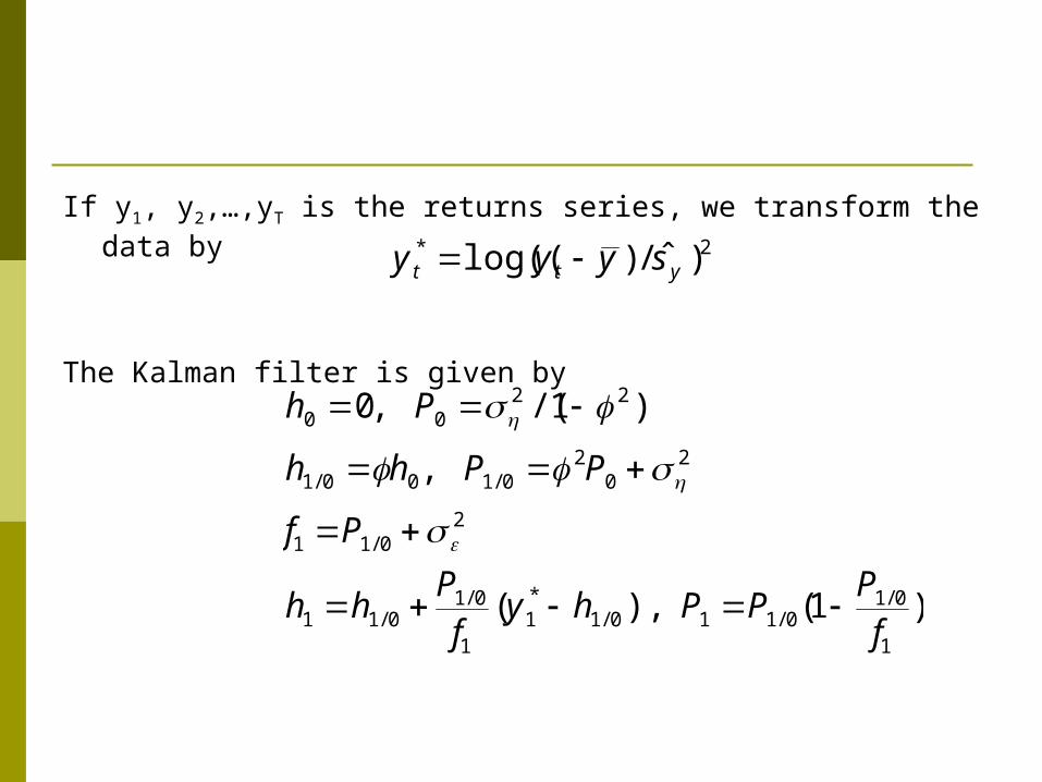
If y1, y2,…,yT is the returns series, we transform the data by

The Kalman filter is given by

2)ˆ/)log((*ytt syyy

)(),(

,

)/(,

///

*//

/

//

1

01011011

1

01011

2011

20

201001

2200

1

10

fP

PPhyfP

hh

Pf

PPhh

Ph

SP500

-25

-20

-15

-10

-5

0

5

10

2500 5000 7500 10000

SP500

5720

17195

00850

99430

2

1200

2

0010

2

0010

.ˆ

.ˆ

.ˆ

.ˆ

*

).(

).(

).(

0.0

0.4

0.8

1.2

1.6

2.0

2.4

2500 5000 7500 10000

VOLSP

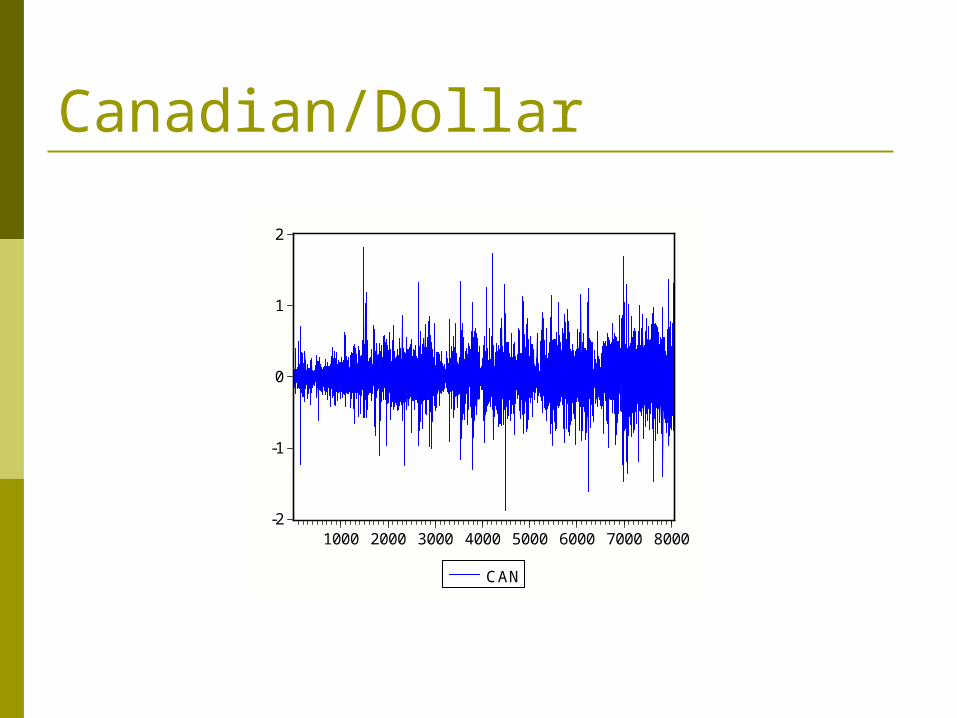
Canadian/Dollar

-2

-1

0

1

2

1000 2000 3000 4000 5000 6000 7000 8000

CAN

0490

2605

0230

9880

2

1400

2

0030

2

0040

.ˆ

.ˆ

.ˆ

.ˆ

*

).(

).(

).(

.0

.1

.2

.3

.4

.5

.6

1000 2000 3000 4000 5000 6000

VOLCAN

Unobserved heteroscedastic componentsUnobserved component models with heteroscedastic

disturbances have been extensively used in the analysis of financial time series; for example, multivariate models with common factors where both the idiosyncratic and common factors may be heteroscedastic as in Harvey, Ruiz and Sentana (1992) or univariate models where the components may be heteroscedastic as in Broto and Ruiz (2005b).

To simplify the exposition, we are focusing on the random walk plus noise model with ARCH(1) disturbances given by

where

ttt

ttty

1

2110

2110

ttttt

ttttt

qq

hh

,

,

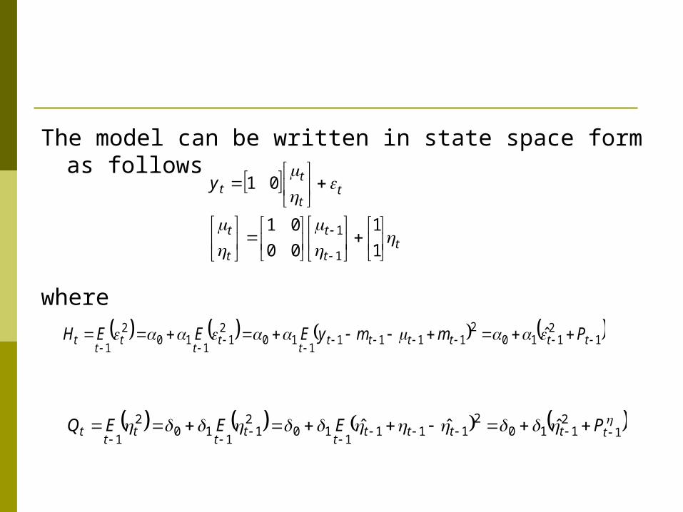
The model can be written in state space form as follows

where

tt

t

t

t

tt

tty

1

1

00

01

01

1

1

12110

21111

110

21

110

2

1

tttttt

tt

tt

tt PmmyEEEH ˆ

12110

2111

110

21

110

2

1

ttttt

tt

tt

tt PEEEQ ˆˆˆ

The model is not conditionally Gaussian, since knowledge of past observations does not, in general, imply knowledge of past disturbances. Nevertheless we can proceed on the basis that the model can be treated as though it were conditionally Gaussian, and we will refer to the Kalman filter as being quasi-optimal.

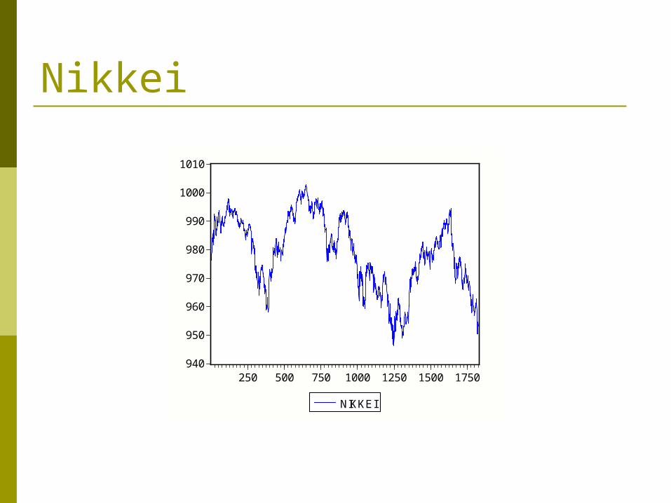
Nikkei

940

950

960

970

980

990

1000

1010

250 500 750 1000 1250 1500 1750

NIKKEI

QML estimates of the Random walk plus noise parameters:

Diagnostics of innovations

4821

11102

2

.ˆ

.ˆ

*.)(

.)(

7814510

8921510

2

Q

Q

-.04

.00

.04

.08

.12

.16

.20

5 10 15 20 25 30 35

DIFIRRENIK DIFFLEVELNIK SDNIKKEI

Diagnostics of auxiliary residuals

*

*

*

*

.)(

.)(

.)(

.)(

8114810

8052310

7040110

6740810

2

2

Q

Q

Q

Q

19494

21

75251

21

08254683

3962

1080900008200350

0790

tttt

t

qq

h

).().().().(

).(

....

.

Hewlett Packard

200

240

280

320

360

400

440

500 1000 1500 2000

HP

QML estimates of the Random walk plus noise parameters:

Diagnostics of innovations

*.)(

.)(

5419310

8982010

2

Q

Q

3527

21502

2

.ˆ

.ˆ

.02

.04

.06

.08

.10

.12

.14

.16

5 10 15 20 25 30 35

DIFIRREHP DIFLEVELHP SDHP

Diagnostics of auxiliary residuals

*

*

*

*

.)(

.)(

.)(

.)(

7319610

8722210

7043110

3951510

2

2

Q

Q

Q

Q

12742

21

257193

21

88648962

1863

0530973002100330

3990

tttt

t

qq

h

).().().().(

).(

....

.