CHAPTER 2 THE SOURCES OF ECONOMIC GROWTHunleashingcapitalismsc.org/pdf/Chapter2.pdfTHE SOURCES OF...
28
CHAPTER 2 by Russell S. Sobel and Joshua C. Hall THE SOURCES OF ECONOMIC GROWTH 21
Transcript of CHAPTER 2 THE SOURCES OF ECONOMIC GROWTHunleashingcapitalismsc.org/pdf/Chapter2.pdfTHE SOURCES OF...
C H A P T E R 2
by Russell S. Sobel and Joshua C. Hall
T H E S O U R C E S O FE C O N O M I C G R O W T H
UNLEASHING CAPITALISM
REFERENCES
Bureau of Economic Analysis, U.S. Department of Commerce. 2009. Annual State Personal
Income [electronic file]. Washington, DC: U.S. Department of Commerce. Online: http://www.bea.gov/regional/spi/default.cfm?selTable=SA30 (cited: August 22, 2009).
Federal Bureau of Investigation, U.S. Department of Justice. 2005. Crime in the United States
2004. Washington DC: Government Printing Office. Heston, Alan, and Robert Summers. 1994. The Penn World Tables (Mark 5.6) [electronic
file]. Cambridge, MA: National Bureau of Economic Research. Morgan, Scott, and Kathleen O'Leary Morgan (eds.). 2009. Health Care State Rankings 2009.
Washington DC: CQ Press. Sobel, Russell S. and Susane J. Daniels. 2007.The Case for Growth, Chapter 1 in Russell S.
Sobel (ed.), Unleashing Capitalism: Why Prosperity Stops at the West Virginia Border and How to Fix It. Morgantown, WV: Center for Economic Growth, The Public Policy Foundation of West Virginia, pp. 1-12.
U.S. Census Bureau. 2004. Education Attainment in the United States 2004 [electronic file]. Washington, DC: U.S. Census Bureau. Online: www.census.gov/population/www/ socdemo/education/cps2004.html (cited: December 22, 2006).
U.S. Census Bureau. 2005. Interim State Population Projections [electronic file]. Washington, DC: U.S. Census Bureau. Online: www.census.gov/population/ projections/MethTab2.xls (cited: December 22, 2006).
U.S. Census Bureau. 2006. Statistical Abstract of the United States, 2006 [electronic file]. Washington, DC: U.S. Census Bureau. Online: www.census.gov/compendia/ statab/2006/2006edition.html (cited: December 22, 2006).
World Bank. 2004. World Development Indicators [CD-ROM].
UNLEASHING CAPITALISM 18
manufacturing property tax in the country. In Figure 5.8 we present the effective property tax rates data for Southeastern states, for comparison. The ranks given for the states are out of all 50 states. The ‘net tax’ and ‘effective tax rate’ are calculated based on property valued at $25 million ($12.5 million in machinery and equipment, $12.5 million in inventories, and $2.5 million in fixtures). Notice that South Carolina’s effective tax rate on industrial property is over 7.8 times higher than the most industry-friendly state, Delaware. (Delaware is listed in the figure because it is the lowest-tax state.)
Figure 5.8: Industrial Property Taxes in Southeastern states*, 2007 State Rank (of 50) Net Tax Effective Tax Rate
South Carolina 1 $1,864,900 3.73%
Mississippi 4 $1,291,050 2.58%
Texas 6 $1,264,358 2.53%
Tennessee 10 $1,033,544 2.07%
West Virginia 14 $833,234 1.67%
Louisiana 17 $783,407 1.57%
Georgia 20 $760,381 1.52%
Florida 24 $677,683 1.36%
Alabama 35 $533,776 1.11%
North Carolina 37 $491,071 0.98%
Kentucky 47 $327,100 0.65%
Virginia 49 $241,498 0.48%
Delaware 50 $238,840 0.48%
Source: National Association of Manufacturers (2009) * Taxes measured in the states’ largest city only.
Importantly, South Carolina’s effective tax rate is almost 2.5 times greater than Georgia’s tax, and almost 4 times greater than North Carolina’s. This puts South Carolina at a serious disadvantage, in terms of its ability to attract and keep industry. Since South Carolina has the highest tax in the country on industrial property, it should be no surprise that it has one of the lowest per capita incomes and economic growth rates in the country. Although it is probably not critical that South Carolina set its tax rate to the lowest in the country, it should definitely make it at least competitive for the Southeast. Since Georgia’s rate is effectively 1.52 percent and North Carolina’s is just under 1 percent, a rate at around 1 percent might be sufficient to attract more industry. Working to reduce the various taxes applied to industry would seriously improve the state’s competitiveness. Such a significant reduction in taxes on industrial property would obviously lead to a reduction in tax revenues on industrial property, at least initially. However, the overall revenue may in fact increase once the growth rate in the state begins to pick up and more industry moves into the state. Furthermore, if the official tax rates are lowered, then the state
21CHAPTER 5: SPECIFIC TAX REFORMS
13
Presumably the original intent of imposing a tax rate schedule with graduated marginal tax rates was to make the income tax progressive. However, what progressivity exists in the state’s income tax structure is due to the zero tax on the first $2,630 of income, and because of the graduated marginal tax rates. However, since the marginal tax rate increases over such small steps in income, as shown in Figure 5.5, most of the progressivity occurs at lower income levels, not higher levels of income. At higher income levels, the average tax rate hardly increases at all. This nature of the current tax is directly contradictory to the goal of progressivity. So although on the surface it appears that the tax satisfies the vertical equity condition, it really does this only at the lower income levels reducing the wealth of these lowest income taxpayers, not the intended consequence.
Figure 5.5: South Carolina income tax: Current tax rates compared to inflation-indexed rates, 2009
Current Income Tax
Rates/Brackets
Income Tax Rates/Brackets if 1959 Tax Schedule was Inflation Adjusted to
2009
Taxable Income Tax
Amount Average Tax Rate
Tax Amount
Average Tax Rate
$5,000 $71 1.42% $125 2.5%
$10,000 $290 2.90% $250 2.5%
$15,000 $604 4.03% $377 2.51%
$20,000 $954 4.77% $527 2.63%
$30,000 $1,654 5.51% $834 2.78%
$50,000 $3,054 6.10% $1,695 3.39%
$75,000 $4,804 6.41% $3,127 4.17%
$100,000 $6,554 6.56% $4,877 4.88%
$150,000 $10,054 6.70% $8,377 5.58%
$200,000 $13,554 6.77% $11,877 5.94%
Figure 5.5 also shows what the average tax rates are for various incomes and taxes
under the current tax system in South Carolina. In the right columns it also shows what the taxes and average tax rates would be if the 1959 tax tables were indexed for inflation. The figure clearly shows that the 1959 indexed tax rate structure is more uniformly progressive, especially at higher levels of incomes. It keeps tax rates extremely low for the lowest income individuals in the state. Figure 5.5 also shows that the current tax system charges all income groups more in taxes than an indexed rate schedule. The only exception is the $5,000 income earner in the table. As South Carolina income taxes continue to climb while the tax brackets remain stagnant, the state becomes a relatively high-tax state. This has a negative impact on

2
THE SOURCES OF ECONOMIC GROWTH
Russell S. Sobel and Joshua C. Hall
The previous chapter made the case for why increasing the rate of economic growth in South Carolina should be considered one of the top policy priorities. However, policy reform to promote growth should be based on evidence of what has worked, and what has not worked in South Carolina and other areas. Evidence was presented in the previous chapter that economic growth is faster in states like Texas, South Dakota, Wyoming, and Louisiana; and in countries like Hong Kong, Japan, and recently Ireland. How can this be replicated in South Carolina? Can we uncover which policies tend to promote prosperity? These are the questions we address in this chapter.1
As we will soon see, there is one thing that high-income and fast-growth places generally have in common: they have unleashed capitalism and backed it up with sound political and legal systems that firmly protect property rights and prohibit fraud, theft, and coercion. By doing so, they have created a level playing field for prosperity to take root. As economist Dwight Lee writes:
No matter how fertile the seeds of entrepreneurship, they wither without the proper economic soil. In order for entrepreneurship to germinate, take root, and yield the fruit of economic progress it has to be nourished by the right mixture of freedom and accountability, a mixture that can only be provided by a free market economy. (1991, 20)
THE PROCESS OF ECONOMIC GROWTH
To understand economic growth and the best way for government policy to promote it, we must first delve deeper into the relationship between economic inputs, institutions, and outcomes.
An economy is a process by which economic inputs and resources, such as skilled labor, capital, and funding for new businesses, are converted into economic outcomes (e.g.,
1 This chapter is based on Sobel and Hall (2007).
UNLEASHING CAPITALISM 18
manufacturing property tax in the country. In Figure 5.8 we present the effective property tax rates data for Southeastern states, for comparison. The ranks given for the states are out of all 50 states. The ‘net tax’ and ‘effective tax rate’ are calculated based on property valued at $25 million ($12.5 million in machinery and equipment, $12.5 million in inventories, and $2.5 million in fixtures). Notice that South Carolina’s effective tax rate on industrial property is over 7.8 times higher than the most industry-friendly state, Delaware. (Delaware is listed in the figure because it is the lowest-tax state.)
Figure 5.8: Industrial Property Taxes in Southeastern states*, 2007 State Rank (of 50) Net Tax Effective Tax Rate
South Carolina 1 $1,864,900 3.73%
Mississippi 4 $1,291,050 2.58%
Texas 6 $1,264,358 2.53%
Tennessee 10 $1,033,544 2.07%
West Virginia 14 $833,234 1.67%
Louisiana 17 $783,407 1.57%
Georgia 20 $760,381 1.52%
Florida 24 $677,683 1.36%
Alabama 35 $533,776 1.11%
North Carolina 37 $491,071 0.98%
Kentucky 47 $327,100 0.65%
Virginia 49 $241,498 0.48%
Delaware 50 $238,840 0.48%
Source: National Association of Manufacturers (2009) * Taxes measured in the states’ largest city only.
Importantly, South Carolina’s effective tax rate is almost 2.5 times greater than Georgia’s tax, and almost 4 times greater than North Carolina’s. This puts South Carolina at a serious disadvantage, in terms of its ability to attract and keep industry. Since South Carolina has the highest tax in the country on industrial property, it should be no surprise that it has one of the lowest per capita incomes and economic growth rates in the country. Although it is probably not critical that South Carolina set its tax rate to the lowest in the country, it should definitely make it at least competitive for the Southeast. Since Georgia’s rate is effectively 1.52 percent and North Carolina’s is just under 1 percent, a rate at around 1 percent might be sufficient to attract more industry. Working to reduce the various taxes applied to industry would seriously improve the state’s competitiveness. Such a significant reduction in taxes on industrial property would obviously lead to a reduction in tax revenues on industrial property, at least initially. However, the overall revenue may in fact increase once the growth rate in the state begins to pick up and more industry moves into the state. Furthermore, if the official tax rates are lowered, then the state
22 CHAPTER 5: SPECIFIC TAX REFORMS
13
Presumably the original intent of imposing a tax rate schedule with graduated marginal tax rates was to make the income tax progressive. However, what progressivity exists in the state’s income tax structure is due to the zero tax on the first $2,630 of income, and because of the graduated marginal tax rates. However, since the marginal tax rate increases over such small steps in income, as shown in Figure 5.5, most of the progressivity occurs at lower income levels, not higher levels of income. At higher income levels, the average tax rate hardly increases at all. This nature of the current tax is directly contradictory to the goal of progressivity. So although on the surface it appears that the tax satisfies the vertical equity condition, it really does this only at the lower income levels reducing the wealth of these lowest income taxpayers, not the intended consequence.
Figure 5.5: South Carolina income tax: Current tax rates compared to inflation-indexed rates, 2009
Current Income Tax
Rates/Brackets
Income Tax Rates/Brackets if 1959 Tax Schedule was Inflation Adjusted to
2009
Taxable Income Tax
Amount Average Tax Rate
Tax Amount
Average Tax Rate
$5,000 $71 1.42% $125 2.5%
$10,000 $290 2.90% $250 2.5%
$15,000 $604 4.03% $377 2.51%
$20,000 $954 4.77% $527 2.63%
$30,000 $1,654 5.51% $834 2.78%
$50,000 $3,054 6.10% $1,695 3.39%
$75,000 $4,804 6.41% $3,127 4.17%
$100,000 $6,554 6.56% $4,877 4.88%
$150,000 $10,054 6.70% $8,377 5.58%
$200,000 $13,554 6.77% $11,877 5.94%
Figure 5.5 also shows what the average tax rates are for various incomes and taxes
under the current tax system in South Carolina. In the right columns it also shows what the taxes and average tax rates would be if the 1959 tax tables were indexed for inflation. The figure clearly shows that the 1959 indexed tax rate structure is more uniformly progressive, especially at higher levels of incomes. It keeps tax rates extremely low for the lowest income individuals in the state. Figure 5.5 also shows that the current tax system charges all income groups more in taxes than an indexed rate schedule. The only exception is the $5,000 income earner in the table. As South Carolina income taxes continue to climb while the tax brackets remain stagnant, the state becomes a relatively high-tax state. This has a negative impact on
UNLEASHING CAPITALISM 18
manufacturing property tax in the country. In Figure 5.8 we present the effective property tax rates data for Southeastern states, for comparison. The ranks given for the states are out of all 50 states. The ‘net tax’ and ‘effective tax rate’ are calculated based on property valued at $25 million ($12.5 million in machinery and equipment, $12.5 million in inventories, and $2.5 million in fixtures). Notice that South Carolina’s effective tax rate on industrial property is over 7.8 times higher than the most industry-friendly state, Delaware. (Delaware is listed in the figure because it is the lowest-tax state.)
Figure 5.8: Industrial Property Taxes in Southeastern states*, 2007 State Rank (of 50) Net Tax Effective Tax Rate
South Carolina 1 $1,864,900 3.73%
Mississippi 4 $1,291,050 2.58%
Texas 6 $1,264,358 2.53%
Tennessee 10 $1,033,544 2.07%
West Virginia 14 $833,234 1.67%
Louisiana 17 $783,407 1.57%
Georgia 20 $760,381 1.52%
Florida 24 $677,683 1.36%
Alabama 35 $533,776 1.11%
North Carolina 37 $491,071 0.98%
Kentucky 47 $327,100 0.65%
Virginia 49 $241,498 0.48%
Delaware 50 $238,840 0.48%
Source: National Association of Manufacturers (2009) * Taxes measured in the states’ largest city only.
Importantly, South Carolina’s effective tax rate is almost 2.5 times greater than Georgia’s tax, and almost 4 times greater than North Carolina’s. This puts South Carolina at a serious disadvantage, in terms of its ability to attract and keep industry. Since South Carolina has the highest tax in the country on industrial property, it should be no surprise that it has one of the lowest per capita incomes and economic growth rates in the country. Although it is probably not critical that South Carolina set its tax rate to the lowest in the country, it should definitely make it at least competitive for the Southeast. Since Georgia’s rate is effectively 1.52 percent and North Carolina’s is just under 1 percent, a rate at around 1 percent might be sufficient to attract more industry. Working to reduce the various taxes applied to industry would seriously improve the state’s competitiveness. Such a significant reduction in taxes on industrial property would obviously lead to a reduction in tax revenues on industrial property, at least initially. However, the overall revenue may in fact increase once the growth rate in the state begins to pick up and more industry moves into the state. Furthermore, if the official tax rates are lowered, then the state
2
THE SOURCES OF ECONOMIC GROWTH
Russell S. Sobel and Joshua C. Hall
The previous chapter made the case for why increasing the rate of economic growth in South Carolina should be considered one of the top policy priorities. However, policy reform to promote growth should be based on evidence of what has worked, and what has not worked in South Carolina and other areas. Evidence was presented in the previous chapter that economic growth is faster in states like Texas, South Dakota, Wyoming, and Louisiana; and in countries like Hong Kong, Japan, and recently Ireland. How can this be replicated in South Carolina? Can we uncover which policies tend to promote prosperity? These are the questions we address in this chapter.1
As we will soon see, there is one thing that high-income and fast-growth places generally have in common: they have unleashed capitalism and backed it up with sound political and legal systems that firmly protect property rights and prohibit fraud, theft, and coercion. By doing so, they have created a level playing field for prosperity to take root. As economist Dwight Lee writes:
No matter how fertile the seeds of entrepreneurship, they wither without the proper economic soil. In order for entrepreneurship to germinate, take root, and yield the fruit of economic progress it has to be nourished by the right mixture of freedom and accountability, a mixture that can only be provided by a free market economy. (1991, 20)
THE PROCESS OF ECONOMIC GROWTH
To understand economic growth and the best way for government policy to promote it, we must first delve deeper into the relationship between economic inputs, institutions, and outcomes.
An economy is a process by which economic inputs and resources, such as skilled labor, capital, and funding for new businesses, are converted into economic outcomes (e.g.,
1 This chapter is based on Sobel and Hall (2007).
UNLEASHING CAPITALISM 18
manufacturing property tax in the country. In Figure 5.8 we present the effective property tax rates data for Southeastern states, for comparison. The ranks given for the states are out of all 50 states. The ‘net tax’ and ‘effective tax rate’ are calculated based on property valued at $25 million ($12.5 million in machinery and equipment, $12.5 million in inventories, and $2.5 million in fixtures). Notice that South Carolina’s effective tax rate on industrial property is over 7.8 times higher than the most industry-friendly state, Delaware. (Delaware is listed in the figure because it is the lowest-tax state.)
Figure 5.8: Industrial Property Taxes in Southeastern states*, 2007 State Rank (of 50) Net Tax Effective Tax Rate
South Carolina 1 $1,864,900 3.73%
Mississippi 4 $1,291,050 2.58%
Texas 6 $1,264,358 2.53%
Tennessee 10 $1,033,544 2.07%
West Virginia 14 $833,234 1.67%
Louisiana 17 $783,407 1.57%
Georgia 20 $760,381 1.52%
Florida 24 $677,683 1.36%
Alabama 35 $533,776 1.11%
North Carolina 37 $491,071 0.98%
Kentucky 47 $327,100 0.65%
Virginia 49 $241,498 0.48%
Delaware 50 $238,840 0.48%
Source: National Association of Manufacturers (2009) * Taxes measured in the states’ largest city only.
Importantly, South Carolina’s effective tax rate is almost 2.5 times greater than Georgia’s tax, and almost 4 times greater than North Carolina’s. This puts South Carolina at a serious disadvantage, in terms of its ability to attract and keep industry. Since South Carolina has the highest tax in the country on industrial property, it should be no surprise that it has one of the lowest per capita incomes and economic growth rates in the country. Although it is probably not critical that South Carolina set its tax rate to the lowest in the country, it should definitely make it at least competitive for the Southeast. Since Georgia’s rate is effectively 1.52 percent and North Carolina’s is just under 1 percent, a rate at around 1 percent might be sufficient to attract more industry. Working to reduce the various taxes applied to industry would seriously improve the state’s competitiveness. Such a significant reduction in taxes on industrial property would obviously lead to a reduction in tax revenues on industrial property, at least initially. However, the overall revenue may in fact increase once the growth rate in the state begins to pick up and more industry moves into the state. Furthermore, if the official tax rates are lowered, then the state
23CHAPTER 5: SPECIFIC TAX REFORMS
13
Presumably the original intent of imposing a tax rate schedule with graduated marginal tax rates was to make the income tax progressive. However, what progressivity exists in the state’s income tax structure is due to the zero tax on the first $2,630 of income, and because of the graduated marginal tax rates. However, since the marginal tax rate increases over such small steps in income, as shown in Figure 5.5, most of the progressivity occurs at lower income levels, not higher levels of income. At higher income levels, the average tax rate hardly increases at all. This nature of the current tax is directly contradictory to the goal of progressivity. So although on the surface it appears that the tax satisfies the vertical equity condition, it really does this only at the lower income levels reducing the wealth of these lowest income taxpayers, not the intended consequence.
Figure 5.5: South Carolina income tax: Current tax rates compared to inflation-indexed rates, 2009
Current Income Tax
Rates/Brackets
Income Tax Rates/Brackets if 1959 Tax Schedule was Inflation Adjusted to
2009
Taxable Income Tax
Amount Average Tax Rate
Tax Amount
Average Tax Rate
$5,000 $71 1.42% $125 2.5%
$10,000 $290 2.90% $250 2.5%
$15,000 $604 4.03% $377 2.51%
$20,000 $954 4.77% $527 2.63%
$30,000 $1,654 5.51% $834 2.78%
$50,000 $3,054 6.10% $1,695 3.39%
$75,000 $4,804 6.41% $3,127 4.17%
$100,000 $6,554 6.56% $4,877 4.88%
$150,000 $10,054 6.70% $8,377 5.58%
$200,000 $13,554 6.77% $11,877 5.94%
Figure 5.5 also shows what the average tax rates are for various incomes and taxes
under the current tax system in South Carolina. In the right columns it also shows what the taxes and average tax rates would be if the 1959 tax tables were indexed for inflation. The figure clearly shows that the 1959 indexed tax rate structure is more uniformly progressive, especially at higher levels of incomes. It keeps tax rates extremely low for the lowest income individuals in the state. Figure 5.5 also shows that the current tax system charges all income groups more in taxes than an indexed rate schedule. The only exception is the $5,000 income earner in the table. As South Carolina income taxes continue to climb while the tax brackets remain stagnant, the state becomes a relatively high-tax state. This has a negative impact on
UNLEASHING CAPITALISM
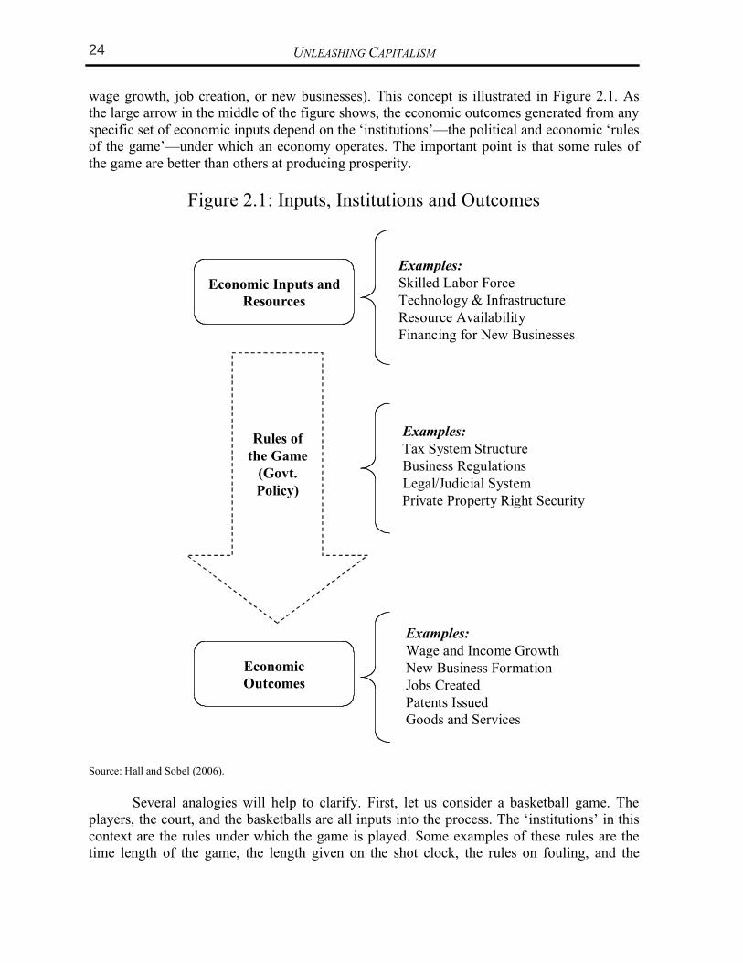
wage growth, job creation, or new businesses). This concept is illustrated in Figure 2.1. As the large arrow in the middle of the figure shows, the economic outcomes generated from any specific set of economic inputs depend on the ‘institutions’—the political and economic ‘rules of the game’—under which an economy operates. The important point is that some rules of the game are better than others at producing prosperity.
Figure 2.1: Inputs, Institutions and Outcomes
Examples:
Skilled Labor Force
Technology & Infrastructure
Resource Availability
Financing for New Businesses
Economic
Outcomes
Examples:
Wage and Income Growth
New Business Formation
Jobs Created
Patents Issued
Goods and Services
Rules of
the Game
(Govt.
Policy)
Economic Inputs and
Resources
Examples:
Tax System Structure
Business Regulations
Legal/Judicial System
Private Property Right Security
Source: Hall and Sobel (2006).
Several analogies will help to clarify. First, let us consider a basketball game. The players, the court, and the basketballs are all inputs into the process. The ‘institutions’ in this context are the rules under which the game is played. Some examples of these rules are the time length of the game, the length given on the shot clock, the rules on fouling, and the
CHAPTER 2: THE SOURCES OF ECONOMIC GROWTH
three-point line rule. Examples of the measurable outcomes are the score, the winning team, the number of fouls, etc. The important point is that the outcomes will be influenced by which rules of the game are chosen. The reason for this is that the rules of the game affect the choices and behavior of the people playing the game. If, for example, the rule that shots made from behind the three point line were changed so that these were now worth only one and a half points, we would expect players to respond to this rule change in a predictable manner. As the point value of those longer shots decreased, fewer players would attempt them.2
While a basketball example might sound hypothetical, Clemson University economists Robert McCormick and Robert Tollison (1984) found that while adding an additional referee to a basketball game was expected to result in more fouls being called, a slower-paced game, and less scoring, when these rule changes were actually introduced in ACC basketball they had precisely the opposite effect. The result was fewer fouls, a faster pace, and more scoring. The explanation? Knowing that fouls were more likely to be called by referees, players changed their behavior and committed fewer of them. To take another example, consider for a moment the board game ‘Monopoly.’ The ‘institutions’ in this analogy are again the rules under which the game is played. Imagine if a new rule were created making it legitimate to steal the property cards of other players if they were not looking. The play and outcomes from a game of ‘Monopoly’ would be significantly different under these different institutional rules, as players would alter their behavior in response to them. Not only would this rule change increase the rate of theft among players, it would also result in fewer properties being purchased, less investment (houses or hotels) on the properties, and more resources being devoted to trying to protect their property cards from being stolen (and more effort into trying to steal the property of other players). As a final analogy, consider the process of baking cakes. In this context, the ingredients are the inputs, the ‘institutions’ are the oven, and the outcomes are the delicious cakes that result at the end. The main point is obvious—if the oven is not working, simply putting more ingredients (inputs) into the oven does not result in more cakes coming out the other end. Too many government policies at every level of government fail to realize this, and keep pouring money into programs that attempt to increase the inputs into the economy when the real problem is that the oven is broken due to failed economic policies. An economy cannot spend its way out of problems that are caused by weak institutions. Rather institutions must be improved, and this, and only this, will result in investments in inputs paying dividends at the other end of the process. This model makes it clear that by improving institutions, or the rules of the game under which the South Carolina economy operates, it can change economic outcomes for the better. When institutions are weak, even places with abundant natural resources or other inputs have difficulty becoming prosperous. South Carolina, and the countries of Argentina and Venezuela, fit into this category of resource-rich areas that have not been able to sustain economic growth (as was noted in the previous chapter). The important point is that our daily economic lives are played out under a set of rules that are to a large extent determined by government-enacted laws and policies. These political and legal ‘institutions’ as economists call them, are what create the incentive structures within the state economy. Prosperity requires that South Carolina get the rules right.
2 This change in the rules would also alter the incentives in the selection of players, or investments in resources
for an economy. Coaches would now have a much weaker preference for players who could make longer shots.
UNLEASHING CAPITALISM 18
manufacturing property tax in the country. In Figure 5.8 we present the effective property tax rates data for Southeastern states, for comparison. The ranks given for the states are out of all 50 states. The ‘net tax’ and ‘effective tax rate’ are calculated based on property valued at $25 million ($12.5 million in machinery and equipment, $12.5 million in inventories, and $2.5 million in fixtures). Notice that South Carolina’s effective tax rate on industrial property is over 7.8 times higher than the most industry-friendly state, Delaware. (Delaware is listed in the figure because it is the lowest-tax state.)
Figure 5.8: Industrial Property Taxes in Southeastern states*, 2007 State Rank (of 50) Net Tax Effective Tax Rate
South Carolina 1 $1,864,900 3.73%
Mississippi 4 $1,291,050 2.58%
Texas 6 $1,264,358 2.53%
Tennessee 10 $1,033,544 2.07%
West Virginia 14 $833,234 1.67%
Louisiana 17 $783,407 1.57%
Georgia 20 $760,381 1.52%
Florida 24 $677,683 1.36%
Alabama 35 $533,776 1.11%
North Carolina 37 $491,071 0.98%
Kentucky 47 $327,100 0.65%
Virginia 49 $241,498 0.48%
Delaware 50 $238,840 0.48%
Source: National Association of Manufacturers (2009) * Taxes measured in the states’ largest city only.
Importantly, South Carolina’s effective tax rate is almost 2.5 times greater than Georgia’s tax, and almost 4 times greater than North Carolina’s. This puts South Carolina at a serious disadvantage, in terms of its ability to attract and keep industry. Since South Carolina has the highest tax in the country on industrial property, it should be no surprise that it has one of the lowest per capita incomes and economic growth rates in the country. Although it is probably not critical that South Carolina set its tax rate to the lowest in the country, it should definitely make it at least competitive for the Southeast. Since Georgia’s rate is effectively 1.52 percent and North Carolina’s is just under 1 percent, a rate at around 1 percent might be sufficient to attract more industry. Working to reduce the various taxes applied to industry would seriously improve the state’s competitiveness. Such a significant reduction in taxes on industrial property would obviously lead to a reduction in tax revenues on industrial property, at least initially. However, the overall revenue may in fact increase once the growth rate in the state begins to pick up and more industry moves into the state. Furthermore, if the official tax rates are lowered, then the state
24 CHAPTER 5: SPECIFIC TAX REFORMS
13
Presumably the original intent of imposing a tax rate schedule with graduated marginal tax rates was to make the income tax progressive. However, what progressivity exists in the state’s income tax structure is due to the zero tax on the first $2,630 of income, and because of the graduated marginal tax rates. However, since the marginal tax rate increases over such small steps in income, as shown in Figure 5.5, most of the progressivity occurs at lower income levels, not higher levels of income. At higher income levels, the average tax rate hardly increases at all. This nature of the current tax is directly contradictory to the goal of progressivity. So although on the surface it appears that the tax satisfies the vertical equity condition, it really does this only at the lower income levels reducing the wealth of these lowest income taxpayers, not the intended consequence.
Figure 5.5: South Carolina income tax: Current tax rates compared to inflation-indexed rates, 2009
Current Income Tax
Rates/Brackets
Income Tax Rates/Brackets if 1959 Tax Schedule was Inflation Adjusted to
2009
Taxable Income Tax
Amount Average Tax Rate
Tax Amount
Average Tax Rate
$5,000 $71 1.42% $125 2.5%
$10,000 $290 2.90% $250 2.5%
$15,000 $604 4.03% $377 2.51%
$20,000 $954 4.77% $527 2.63%
$30,000 $1,654 5.51% $834 2.78%
$50,000 $3,054 6.10% $1,695 3.39%
$75,000 $4,804 6.41% $3,127 4.17%
$100,000 $6,554 6.56% $4,877 4.88%
$150,000 $10,054 6.70% $8,377 5.58%
$200,000 $13,554 6.77% $11,877 5.94%
Figure 5.5 also shows what the average tax rates are for various incomes and taxes
under the current tax system in South Carolina. In the right columns it also shows what the taxes and average tax rates would be if the 1959 tax tables were indexed for inflation. The figure clearly shows that the 1959 indexed tax rate structure is more uniformly progressive, especially at higher levels of incomes. It keeps tax rates extremely low for the lowest income individuals in the state. Figure 5.5 also shows that the current tax system charges all income groups more in taxes than an indexed rate schedule. The only exception is the $5,000 income earner in the table. As South Carolina income taxes continue to climb while the tax brackets remain stagnant, the state becomes a relatively high-tax state. This has a negative impact on
UNLEASHING CAPITALISM
wage growth, job creation, or new businesses). This concept is illustrated in Figure 2.1. As the large arrow in the middle of the figure shows, the economic outcomes generated from any specific set of economic inputs depend on the ‘institutions’—the political and economic ‘rules of the game’—under which an economy operates. The important point is that some rules of the game are better than others at producing prosperity.
Figure 2.1: Inputs, Institutions and Outcomes
Examples:
Skilled Labor Force
Technology & Infrastructure
Resource Availability
Financing for New Businesses
Economic
Outcomes
Examples:
Wage and Income Growth
New Business Formation
Jobs Created
Patents Issued
Goods and Services
Rules of
the Game
(Govt.
Policy)
Economic Inputs and
Resources
Examples:
Tax System Structure
Business Regulations
Legal/Judicial System
Private Property Right Security
Source: Hall and Sobel (2006).
Several analogies will help to clarify. First, let us consider a basketball game. The players, the court, and the basketballs are all inputs into the process. The ‘institutions’ in this context are the rules under which the game is played. Some examples of these rules are the time length of the game, the length given on the shot clock, the rules on fouling, and the
CHAPTER 2: THE SOURCES OF ECONOMIC GROWTH
three-point line rule. Examples of the measurable outcomes are the score, the winning team, the number of fouls, etc. The important point is that the outcomes will be influenced by which rules of the game are chosen. The reason for this is that the rules of the game affect the choices and behavior of the people playing the game. If, for example, the rule that shots made from behind the three point line were changed so that these were now worth only one and a half points, we would expect players to respond to this rule change in a predictable manner. As the point value of those longer shots decreased, fewer players would attempt them.2
While a basketball example might sound hypothetical, Clemson University economists Robert McCormick and Robert Tollison (1984) found that while adding an additional referee to a basketball game was expected to result in more fouls being called, a slower-paced game, and less scoring, when these rule changes were actually introduced in ACC basketball they had precisely the opposite effect. The result was fewer fouls, a faster pace, and more scoring. The explanation? Knowing that fouls were more likely to be called by referees, players changed their behavior and committed fewer of them. To take another example, consider for a moment the board game ‘Monopoly.’ The ‘institutions’ in this analogy are again the rules under which the game is played. Imagine if a new rule were created making it legitimate to steal the property cards of other players if they were not looking. The play and outcomes from a game of ‘Monopoly’ would be significantly different under these different institutional rules, as players would alter their behavior in response to them. Not only would this rule change increase the rate of theft among players, it would also result in fewer properties being purchased, less investment (houses or hotels) on the properties, and more resources being devoted to trying to protect their property cards from being stolen (and more effort into trying to steal the property of other players). As a final analogy, consider the process of baking cakes. In this context, the ingredients are the inputs, the ‘institutions’ are the oven, and the outcomes are the delicious cakes that result at the end. The main point is obvious—if the oven is not working, simply putting more ingredients (inputs) into the oven does not result in more cakes coming out the other end. Too many government policies at every level of government fail to realize this, and keep pouring money into programs that attempt to increase the inputs into the economy when the real problem is that the oven is broken due to failed economic policies. An economy cannot spend its way out of problems that are caused by weak institutions. Rather institutions must be improved, and this, and only this, will result in investments in inputs paying dividends at the other end of the process. This model makes it clear that by improving institutions, or the rules of the game under which the South Carolina economy operates, it can change economic outcomes for the better. When institutions are weak, even places with abundant natural resources or other inputs have difficulty becoming prosperous. South Carolina, and the countries of Argentina and Venezuela, fit into this category of resource-rich areas that have not been able to sustain economic growth (as was noted in the previous chapter). The important point is that our daily economic lives are played out under a set of rules that are to a large extent determined by government-enacted laws and policies. These political and legal ‘institutions’ as economists call them, are what create the incentive structures within the state economy. Prosperity requires that South Carolina get the rules right.
2 This change in the rules would also alter the incentives in the selection of players, or investments in resources
for an economy. Coaches would now have a much weaker preference for players who could make longer shots.
UNLEASHING CAPITALISM 18
manufacturing property tax in the country. In Figure 5.8 we present the effective property tax rates data for Southeastern states, for comparison. The ranks given for the states are out of all 50 states. The ‘net tax’ and ‘effective tax rate’ are calculated based on property valued at $25 million ($12.5 million in machinery and equipment, $12.5 million in inventories, and $2.5 million in fixtures). Notice that South Carolina’s effective tax rate on industrial property is over 7.8 times higher than the most industry-friendly state, Delaware. (Delaware is listed in the figure because it is the lowest-tax state.)
Figure 5.8: Industrial Property Taxes in Southeastern states*, 2007 State Rank (of 50) Net Tax Effective Tax Rate
South Carolina 1 $1,864,900 3.73%
Mississippi 4 $1,291,050 2.58%
Texas 6 $1,264,358 2.53%
Tennessee 10 $1,033,544 2.07%
West Virginia 14 $833,234 1.67%
Louisiana 17 $783,407 1.57%
Georgia 20 $760,381 1.52%
Florida 24 $677,683 1.36%
Alabama 35 $533,776 1.11%
North Carolina 37 $491,071 0.98%
Kentucky 47 $327,100 0.65%
Virginia 49 $241,498 0.48%
Delaware 50 $238,840 0.48%
Source: National Association of Manufacturers (2009) * Taxes measured in the states’ largest city only.
Importantly, South Carolina’s effective tax rate is almost 2.5 times greater than Georgia’s tax, and almost 4 times greater than North Carolina’s. This puts South Carolina at a serious disadvantage, in terms of its ability to attract and keep industry. Since South Carolina has the highest tax in the country on industrial property, it should be no surprise that it has one of the lowest per capita incomes and economic growth rates in the country. Although it is probably not critical that South Carolina set its tax rate to the lowest in the country, it should definitely make it at least competitive for the Southeast. Since Georgia’s rate is effectively 1.52 percent and North Carolina’s is just under 1 percent, a rate at around 1 percent might be sufficient to attract more industry. Working to reduce the various taxes applied to industry would seriously improve the state’s competitiveness. Such a significant reduction in taxes on industrial property would obviously lead to a reduction in tax revenues on industrial property, at least initially. However, the overall revenue may in fact increase once the growth rate in the state begins to pick up and more industry moves into the state. Furthermore, if the official tax rates are lowered, then the state
25CHAPTER 5: SPECIFIC TAX REFORMS
13
Presumably the original intent of imposing a tax rate schedule with graduated marginal tax rates was to make the income tax progressive. However, what progressivity exists in the state’s income tax structure is due to the zero tax on the first $2,630 of income, and because of the graduated marginal tax rates. However, since the marginal tax rate increases over such small steps in income, as shown in Figure 5.5, most of the progressivity occurs at lower income levels, not higher levels of income. At higher income levels, the average tax rate hardly increases at all. This nature of the current tax is directly contradictory to the goal of progressivity. So although on the surface it appears that the tax satisfies the vertical equity condition, it really does this only at the lower income levels reducing the wealth of these lowest income taxpayers, not the intended consequence.
Figure 5.5: South Carolina income tax: Current tax rates compared to inflation-indexed rates, 2009
Current Income Tax
Rates/Brackets
Income Tax Rates/Brackets if 1959 Tax Schedule was Inflation Adjusted to
2009
Taxable Income Tax
Amount Average Tax Rate
Tax Amount
Average Tax Rate
$5,000 $71 1.42% $125 2.5%
$10,000 $290 2.90% $250 2.5%
$15,000 $604 4.03% $377 2.51%
$20,000 $954 4.77% $527 2.63%
$30,000 $1,654 5.51% $834 2.78%
$50,000 $3,054 6.10% $1,695 3.39%
$75,000 $4,804 6.41% $3,127 4.17%
$100,000 $6,554 6.56% $4,877 4.88%
$150,000 $10,054 6.70% $8,377 5.58%
$200,000 $13,554 6.77% $11,877 5.94%
Figure 5.5 also shows what the average tax rates are for various incomes and taxes
under the current tax system in South Carolina. In the right columns it also shows what the taxes and average tax rates would be if the 1959 tax tables were indexed for inflation. The figure clearly shows that the 1959 indexed tax rate structure is more uniformly progressive, especially at higher levels of incomes. It keeps tax rates extremely low for the lowest income individuals in the state. Figure 5.5 also shows that the current tax system charges all income groups more in taxes than an indexed rate schedule. The only exception is the $5,000 income earner in the table. As South Carolina income taxes continue to climb while the tax brackets remain stagnant, the state becomes a relatively high-tax state. This has a negative impact on
UNLEASHING CAPITALISM
ADAM SMITH’S QUESTION:
WHY ARE SOME PLACES RICH AND OTHERS POOR?
Adam Smith, the ‘father of economics,’ published the first book addressing the set of topics we now consider ‘economics’ in 1776. In his book, titled An Inquiry into the Nature
and Causes of the Wealth of Nations, Adam Smith (1998 [1776]) attempted to answer a single question: Why are some nations rich and others poor? Economic science has come a long way in 200 years, and volumes of published research now clearly provide the answer to the question Adam Smith posed long ago. The answer is fundamentally the same one arrived at by Adam Smith.
In a nutshell, he found that countries become prosperous when they have good institutions that create favorable rules of the game—rules that encourage the creation of wealth. Smith further concluded that the institutional structure that best promotes prosperity is an economic system of capitalism backed up by sound political and legal institutions. According to Smith, an economy becomes prosperous when they use unregulated private markets to the greatest extent possible, with the government playing the important but limited role of protecting liberty, property, and enforcing contracts. More than 200 years of published scientific evidence now supports Smith’s conclusion. Capitalism is not a political position or platform, it is an economic system—a set of institutions or rules that define the ‘economic game.’ Capitalism’s institutions produce prosperity better than the alternative of government control, not only in terms of financial wealth, but in terms of other measures of quality of life. Adopting institutions (‘rules of the game’) consistent with the economic system of capitalism has the potential to generate outcomes that better accomplish the common goals of all political parties: prosperity, wealth, health, family, security, etc.
THE RISE AND DECLINE OF ECONOMIC FREEDOM
IN SOUTH CAROLINA
While most people tend to think of capitalism and socialism as alternative and discrete forms of economic organization, in reality government policies tend to lie somewhere on a continuum between these two extremes. What differs on this continuum is the degree to which the government uses its power to enact command and control policies that intervene into the private sector. Some countries, like North Korea, have governments that use a command and control approach to organizing nearly the entire economy. These countries lie at the extreme socialist end of the capitalist-socialist spectrum. Other countries, such as China, are nominally socialist but rely considerably more on the private sector in organizing their economies. Some countries have moved from one end of the continuum to the other, like the former Soviet Republics of Estonia and Latvia, and Slovenia (formerly part of socialist Yugoslavia), who all adopted radical reforms that moved them toward capitalism. On the other hand, most market-based economies have a much larger degree of government intervention and control than is envisioned under pure capitalism. Within the last decade, a significant advance in our understanding of this continuum was the publication of the Economic Freedom of the World index created by economists James Gwartney (a former
CHAPTER 2: THE SOURCES OF ECONOMIC GROWTH
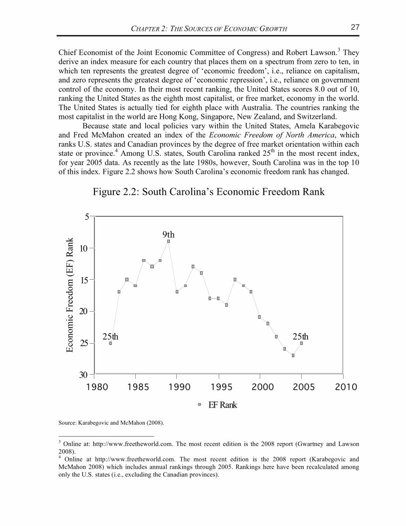
Chief Economist of the Joint Economic Committee of Congress) and Robert Lawson.3 They derive an index measure for each country that places them on a spectrum from zero to ten, in which ten represents the greatest degree of ‘economic freedom’, i.e., reliance on capitalism, and zero represents the greatest degree of ‘economic repression’, i.e., reliance on government control of the economy. In their most recent ranking, the United States scores 8.0 out of 10, ranking the United States as the eighth most capitalist, or free market, economy in the world. The United States is actually tied for eighth place with Australia. The countries ranking the most capitalist in the world are Hong Kong, Singapore, New Zealand, and Switzerland. Because state and local policies vary within the United States, Amela Karabegovic and Fred McMahon created an index of the Economic Freedom of North America, which ranks U.S. states and Canadian provinces by the degree of free market orientation within each state or province.4 Among U.S. states, South Carolina ranked 25th in the most recent index, for year 2005 data. As recently as the late 1980s, however, South Carolina was in the top 10 of this index. Figure 2.2 shows how South Carolina’s economic freedom rank has changed.
Figure 2.2: South Carolina’s Economic Freedom Rank
25th
9th
25th
1980 1985 1990 1995 2000 2005 2010
5
10
15
20
25
30
Eco
no
mic
Fre
edo
m (
EF
) R
ank
EF Rank
Source: Karabegovic and McMahon (2008).
3 Online at: http://www.freetheworld.com. The most recent edition is the 2008 report (Gwartney and Lawson
2008). 4 Online at http://www.freetheworld.com. The most recent edition is the 2008 report (Karabegovic and
McMahon 2008) which includes annual rankings through 2005. Rankings here have been recalculated among
only the U.S. states (i.e., excluding the Canadian provinces).
UNLEASHING CAPITALISM 18
manufacturing property tax in the country. In Figure 5.8 we present the effective property tax rates data for Southeastern states, for comparison. The ranks given for the states are out of all 50 states. The ‘net tax’ and ‘effective tax rate’ are calculated based on property valued at $25 million ($12.5 million in machinery and equipment, $12.5 million in inventories, and $2.5 million in fixtures). Notice that South Carolina’s effective tax rate on industrial property is over 7.8 times higher than the most industry-friendly state, Delaware. (Delaware is listed in the figure because it is the lowest-tax state.)
Figure 5.8: Industrial Property Taxes in Southeastern states*, 2007 State Rank (of 50) Net Tax Effective Tax Rate
South Carolina 1 $1,864,900 3.73%
Mississippi 4 $1,291,050 2.58%
Texas 6 $1,264,358 2.53%
Tennessee 10 $1,033,544 2.07%
West Virginia 14 $833,234 1.67%
Louisiana 17 $783,407 1.57%
Georgia 20 $760,381 1.52%
Florida 24 $677,683 1.36%
Alabama 35 $533,776 1.11%
North Carolina 37 $491,071 0.98%
Kentucky 47 $327,100 0.65%
Virginia 49 $241,498 0.48%
Delaware 50 $238,840 0.48%
Source: National Association of Manufacturers (2009) * Taxes measured in the states’ largest city only.
Importantly, South Carolina’s effective tax rate is almost 2.5 times greater than Georgia’s tax, and almost 4 times greater than North Carolina’s. This puts South Carolina at a serious disadvantage, in terms of its ability to attract and keep industry. Since South Carolina has the highest tax in the country on industrial property, it should be no surprise that it has one of the lowest per capita incomes and economic growth rates in the country. Although it is probably not critical that South Carolina set its tax rate to the lowest in the country, it should definitely make it at least competitive for the Southeast. Since Georgia’s rate is effectively 1.52 percent and North Carolina’s is just under 1 percent, a rate at around 1 percent might be sufficient to attract more industry. Working to reduce the various taxes applied to industry would seriously improve the state’s competitiveness. Such a significant reduction in taxes on industrial property would obviously lead to a reduction in tax revenues on industrial property, at least initially. However, the overall revenue may in fact increase once the growth rate in the state begins to pick up and more industry moves into the state. Furthermore, if the official tax rates are lowered, then the state
26 CHAPTER 5: SPECIFIC TAX REFORMS
13
Presumably the original intent of imposing a tax rate schedule with graduated marginal tax rates was to make the income tax progressive. However, what progressivity exists in the state’s income tax structure is due to the zero tax on the first $2,630 of income, and because of the graduated marginal tax rates. However, since the marginal tax rate increases over such small steps in income, as shown in Figure 5.5, most of the progressivity occurs at lower income levels, not higher levels of income. At higher income levels, the average tax rate hardly increases at all. This nature of the current tax is directly contradictory to the goal of progressivity. So although on the surface it appears that the tax satisfies the vertical equity condition, it really does this only at the lower income levels reducing the wealth of these lowest income taxpayers, not the intended consequence.
Figure 5.5: South Carolina income tax: Current tax rates compared to inflation-indexed rates, 2009
Current Income Tax
Rates/Brackets
Income Tax Rates/Brackets if 1959 Tax Schedule was Inflation Adjusted to
2009
Taxable Income Tax
Amount Average Tax Rate
Tax Amount
Average Tax Rate
$5,000 $71 1.42% $125 2.5%
$10,000 $290 2.90% $250 2.5%
$15,000 $604 4.03% $377 2.51%
$20,000 $954 4.77% $527 2.63%
$30,000 $1,654 5.51% $834 2.78%
$50,000 $3,054 6.10% $1,695 3.39%
$75,000 $4,804 6.41% $3,127 4.17%
$100,000 $6,554 6.56% $4,877 4.88%
$150,000 $10,054 6.70% $8,377 5.58%
$200,000 $13,554 6.77% $11,877 5.94%
Figure 5.5 also shows what the average tax rates are for various incomes and taxes
under the current tax system in South Carolina. In the right columns it also shows what the taxes and average tax rates would be if the 1959 tax tables were indexed for inflation. The figure clearly shows that the 1959 indexed tax rate structure is more uniformly progressive, especially at higher levels of incomes. It keeps tax rates extremely low for the lowest income individuals in the state. Figure 5.5 also shows that the current tax system charges all income groups more in taxes than an indexed rate schedule. The only exception is the $5,000 income earner in the table. As South Carolina income taxes continue to climb while the tax brackets remain stagnant, the state becomes a relatively high-tax state. This has a negative impact on
UNLEASHING CAPITALISM
ADAM SMITH’S QUESTION:
WHY ARE SOME PLACES RICH AND OTHERS POOR?
Adam Smith, the ‘father of economics,’ published the first book addressing the set of topics we now consider ‘economics’ in 1776. In his book, titled An Inquiry into the Nature
and Causes of the Wealth of Nations, Adam Smith (1998 [1776]) attempted to answer a single question: Why are some nations rich and others poor? Economic science has come a long way in 200 years, and volumes of published research now clearly provide the answer to the question Adam Smith posed long ago. The answer is fundamentally the same one arrived at by Adam Smith.
In a nutshell, he found that countries become prosperous when they have good institutions that create favorable rules of the game—rules that encourage the creation of wealth. Smith further concluded that the institutional structure that best promotes prosperity is an economic system of capitalism backed up by sound political and legal institutions. According to Smith, an economy becomes prosperous when they use unregulated private markets to the greatest extent possible, with the government playing the important but limited role of protecting liberty, property, and enforcing contracts. More than 200 years of published scientific evidence now supports Smith’s conclusion. Capitalism is not a political position or platform, it is an economic system—a set of institutions or rules that define the ‘economic game.’ Capitalism’s institutions produce prosperity better than the alternative of government control, not only in terms of financial wealth, but in terms of other measures of quality of life. Adopting institutions (‘rules of the game’) consistent with the economic system of capitalism has the potential to generate outcomes that better accomplish the common goals of all political parties: prosperity, wealth, health, family, security, etc.
THE RISE AND DECLINE OF ECONOMIC FREEDOM
IN SOUTH CAROLINA
While most people tend to think of capitalism and socialism as alternative and discrete forms of economic organization, in reality government policies tend to lie somewhere on a continuum between these two extremes. What differs on this continuum is the degree to which the government uses its power to enact command and control policies that intervene into the private sector. Some countries, like North Korea, have governments that use a command and control approach to organizing nearly the entire economy. These countries lie at the extreme socialist end of the capitalist-socialist spectrum. Other countries, such as China, are nominally socialist but rely considerably more on the private sector in organizing their economies. Some countries have moved from one end of the continuum to the other, like the former Soviet Republics of Estonia and Latvia, and Slovenia (formerly part of socialist Yugoslavia), who all adopted radical reforms that moved them toward capitalism. On the other hand, most market-based economies have a much larger degree of government intervention and control than is envisioned under pure capitalism. Within the last decade, a significant advance in our understanding of this continuum was the publication of the Economic Freedom of the World index created by economists James Gwartney (a former
CHAPTER 2: THE SOURCES OF ECONOMIC GROWTH
Chief Economist of the Joint Economic Committee of Congress) and Robert Lawson.3 They derive an index measure for each country that places them on a spectrum from zero to ten, in which ten represents the greatest degree of ‘economic freedom’, i.e., reliance on capitalism, and zero represents the greatest degree of ‘economic repression’, i.e., reliance on government control of the economy. In their most recent ranking, the United States scores 8.0 out of 10, ranking the United States as the eighth most capitalist, or free market, economy in the world. The United States is actually tied for eighth place with Australia. The countries ranking the most capitalist in the world are Hong Kong, Singapore, New Zealand, and Switzerland. Because state and local policies vary within the United States, Amela Karabegovic and Fred McMahon created an index of the Economic Freedom of North America, which ranks U.S. states and Canadian provinces by the degree of free market orientation within each state or province.4 Among U.S. states, South Carolina ranked 25th in the most recent index, for year 2005 data. As recently as the late 1980s, however, South Carolina was in the top 10 of this index. Figure 2.2 shows how South Carolina’s economic freedom rank has changed.
Figure 2.2: South Carolina’s Economic Freedom Rank
25th
9th
25th
1980 1985 1990 1995 2000 2005 2010
5
10
15
20
25
30
Eco
no
mic
Fre
edo
m (
EF
) R
ank
EF Rank
Source: Karabegovic and McMahon (2008).
3 Online at: http://www.freetheworld.com. The most recent edition is the 2008 report (Gwartney and Lawson
2008). 4 Online at http://www.freetheworld.com. The most recent edition is the 2008 report (Karabegovic and
McMahon 2008) which includes annual rankings through 2005. Rankings here have been recalculated among
only the U.S. states (i.e., excluding the Canadian provinces).
UNLEASHING CAPITALISM 18
manufacturing property tax in the country. In Figure 5.8 we present the effective property tax rates data for Southeastern states, for comparison. The ranks given for the states are out of all 50 states. The ‘net tax’ and ‘effective tax rate’ are calculated based on property valued at $25 million ($12.5 million in machinery and equipment, $12.5 million in inventories, and $2.5 million in fixtures). Notice that South Carolina’s effective tax rate on industrial property is over 7.8 times higher than the most industry-friendly state, Delaware. (Delaware is listed in the figure because it is the lowest-tax state.)
Figure 5.8: Industrial Property Taxes in Southeastern states*, 2007 State Rank (of 50) Net Tax Effective Tax Rate
South Carolina 1 $1,864,900 3.73%
Mississippi 4 $1,291,050 2.58%
Texas 6 $1,264,358 2.53%
Tennessee 10 $1,033,544 2.07%
West Virginia 14 $833,234 1.67%
Louisiana 17 $783,407 1.57%
Georgia 20 $760,381 1.52%
Florida 24 $677,683 1.36%
Alabama 35 $533,776 1.11%
North Carolina 37 $491,071 0.98%
Kentucky 47 $327,100 0.65%
Virginia 49 $241,498 0.48%
Delaware 50 $238,840 0.48%
Source: National Association of Manufacturers (2009) * Taxes measured in the states’ largest city only.
Importantly, South Carolina’s effective tax rate is almost 2.5 times greater than Georgia’s tax, and almost 4 times greater than North Carolina’s. This puts South Carolina at a serious disadvantage, in terms of its ability to attract and keep industry. Since South Carolina has the highest tax in the country on industrial property, it should be no surprise that it has one of the lowest per capita incomes and economic growth rates in the country. Although it is probably not critical that South Carolina set its tax rate to the lowest in the country, it should definitely make it at least competitive for the Southeast. Since Georgia’s rate is effectively 1.52 percent and North Carolina’s is just under 1 percent, a rate at around 1 percent might be sufficient to attract more industry. Working to reduce the various taxes applied to industry would seriously improve the state’s competitiveness. Such a significant reduction in taxes on industrial property would obviously lead to a reduction in tax revenues on industrial property, at least initially. However, the overall revenue may in fact increase once the growth rate in the state begins to pick up and more industry moves into the state. Furthermore, if the official tax rates are lowered, then the state
27CHAPTER 5: SPECIFIC TAX REFORMS
13
Presumably the original intent of imposing a tax rate schedule with graduated marginal tax rates was to make the income tax progressive. However, what progressivity exists in the state’s income tax structure is due to the zero tax on the first $2,630 of income, and because of the graduated marginal tax rates. However, since the marginal tax rate increases over such small steps in income, as shown in Figure 5.5, most of the progressivity occurs at lower income levels, not higher levels of income. At higher income levels, the average tax rate hardly increases at all. This nature of the current tax is directly contradictory to the goal of progressivity. So although on the surface it appears that the tax satisfies the vertical equity condition, it really does this only at the lower income levels reducing the wealth of these lowest income taxpayers, not the intended consequence.
Figure 5.5: South Carolina income tax: Current tax rates compared to inflation-indexed rates, 2009
Current Income Tax
Rates/Brackets
Income Tax Rates/Brackets if 1959 Tax Schedule was Inflation Adjusted to
2009
Taxable Income Tax
Amount Average Tax Rate
Tax Amount
Average Tax Rate
$5,000 $71 1.42% $125 2.5%
$10,000 $290 2.90% $250 2.5%
$15,000 $604 4.03% $377 2.51%
$20,000 $954 4.77% $527 2.63%
$30,000 $1,654 5.51% $834 2.78%
$50,000 $3,054 6.10% $1,695 3.39%
$75,000 $4,804 6.41% $3,127 4.17%
$100,000 $6,554 6.56% $4,877 4.88%
$150,000 $10,054 6.70% $8,377 5.58%
$200,000 $13,554 6.77% $11,877 5.94%
Figure 5.5 also shows what the average tax rates are for various incomes and taxes
under the current tax system in South Carolina. In the right columns it also shows what the taxes and average tax rates would be if the 1959 tax tables were indexed for inflation. The figure clearly shows that the 1959 indexed tax rate structure is more uniformly progressive, especially at higher levels of incomes. It keeps tax rates extremely low for the lowest income individuals in the state. Figure 5.5 also shows that the current tax system charges all income groups more in taxes than an indexed rate schedule. The only exception is the $5,000 income earner in the table. As South Carolina income taxes continue to climb while the tax brackets remain stagnant, the state becomes a relatively high-tax state. This has a negative impact on
UNLEASHING CAPITALISM
During the 1980s, South Carolina rose from 25th to 9th in the economic freedom ranking among U.S. states. In 1989 South Carolina’s policies ranked among the top 10 most free market in the country. Since that time, and particularly since 1997, economic freedom has been on the decline in South Carolina, falling back to where it began in the early 1980s.
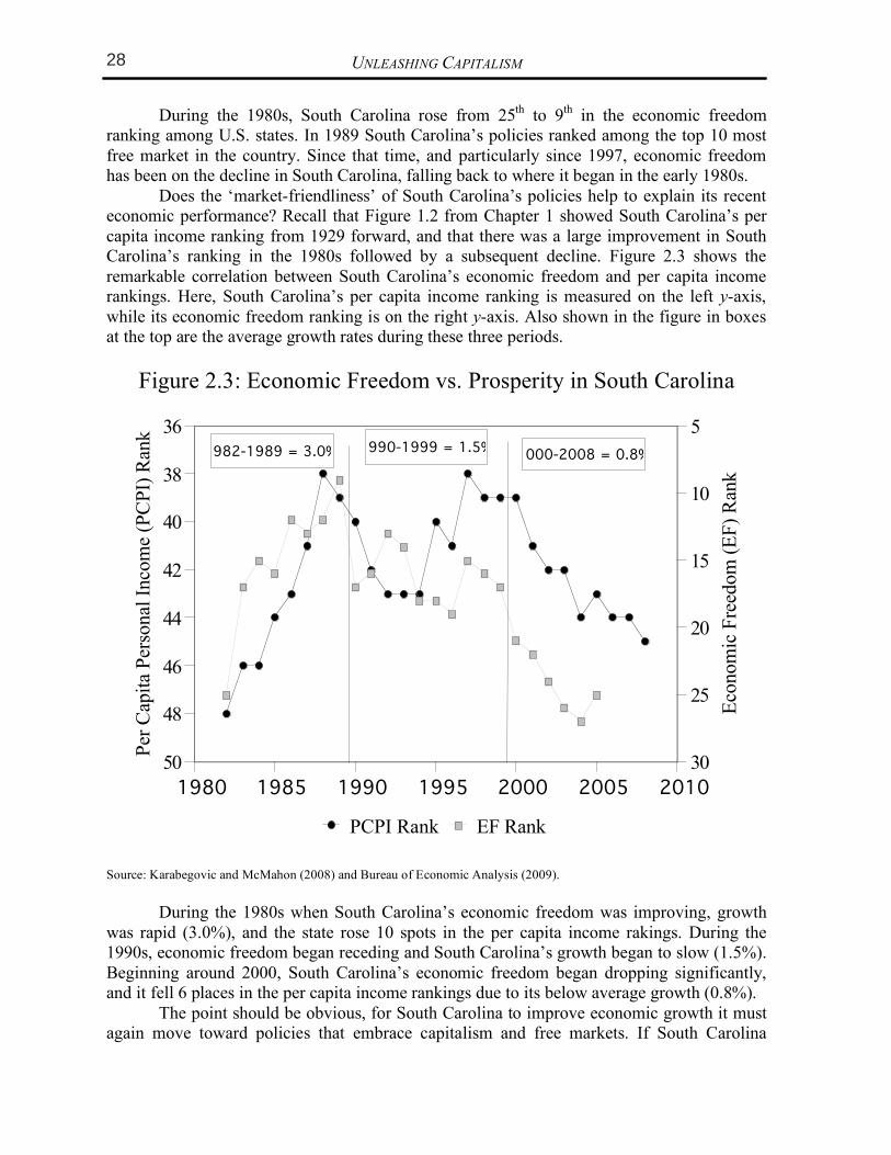
Does the ‘market-friendliness’ of South Carolina’s policies help to explain its recent economic performance? Recall that Figure 1.2 from Chapter 1 showed South Carolina’s per capita income ranking from 1929 forward, and that there was a large improvement in South Carolina’s ranking in the 1980s followed by a subsequent decline. Figure 2.3 shows the remarkable correlation between South Carolina’s economic freedom and per capita income rankings. Here, South Carolina’s per capita income ranking is measured on the left y-axis, while its economic freedom ranking is on the right y-axis. Also shown in the figure in boxes at the top are the average growth rates during these three periods.
Figure 2.3: Economic Freedom vs. Prosperity in South Carolina
1980 1985 1990 1995 2000 2005 2010
36
38
40
42
44
46
48
50
Per
Cap
ita
Per
sonal
Inco
me
(PC
PI)
Ran
k 5
10
15
20
25
30
Eco
nom
ic F
reed
om
(E
F)
Ran
k
PCPI Rank EF Rank
1982-1989 = 3.0% 1990-1999 = 1.5%2000-2008 = 0.8%
Source: Karabegovic and McMahon (2008) and Bureau of Economic Analysis (2009).
During the 1980s when South Carolina’s economic freedom was improving, growth
was rapid (3.0%), and the state rose 10 spots in the per capita income rakings. During the 1990s, economic freedom began receding and South Carolina’s growth began to slow (1.5%). Beginning around 2000, South Carolina’s economic freedom began dropping significantly, and it fell 6 places in the per capita income rankings due to its below average growth (0.8%).
The point should be obvious, for South Carolina to improve economic growth it must again move toward policies that embrace capitalism and free markets. If South Carolina
CHAPTER 2: THE SOURCES OF ECONOMIC GROWTH
continues its current policy trend, the state’s economic ranking is likely to suffer, and within a decade South Carolina will be at the very bottom of the national economic rankings with states such as West Virginia and Mississippi. With all of South Carolina’s advantages over these states, it is almost unbelievable that the Palmetto State could be in such company. Yet, as the earlier oven analogy demonstrated, when policies are bad, economic outcomes suffer despite having good inputs into the process. Returning to Ireland’s growth ‘miracle’ discussed in the previous chapter, we find an example of a country enacting significant pro-market reforms and gaining prosperity as a result. Ireland jumped from a score of 6.3 (out of 10) in 1985 to a score of 8.2 by 1995 in the international economic freedom index, leading Ireland to become the fifth most free market economy in the world. As a result, Ireland’s growth skyrocketed, unemployment fell, and prosperity flourished.
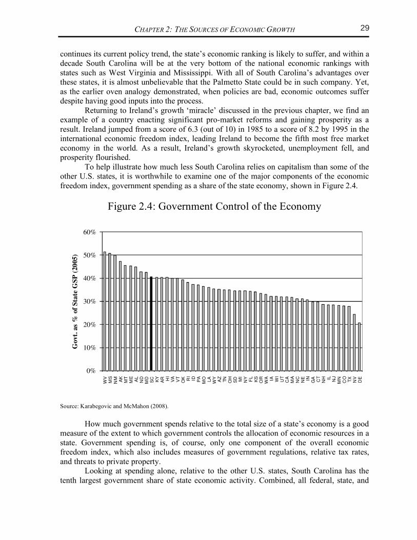
To help illustrate how much less South Carolina relies on capitalism than some of the other U.S. states, it is worthwhile to examine one of the major components of the economic freedom index, government spending as a share of the state economy, shown in Figure 2.4.
Figure 2.4: Government Control of the Economy
0%
10%
20%
30%
40%
50%
60%
Source: Karabegovic and McMahon (2008).
How much government spends relative to the total size of a state’s economy is a good
measure of the extent to which government controls the allocation of economic resources in a state. Government spending is, of course, only one component of the overall economic freedom index, which also includes measures of government regulations, relative tax rates, and threats to private property.
Looking at spending alone, relative to the other U.S. states, South Carolina has the tenth largest government share of state economic activity. Combined, all federal, state, and
UNLEASHING CAPITALISM 18
manufacturing property tax in the country. In Figure 5.8 we present the effective property tax rates data for Southeastern states, for comparison. The ranks given for the states are out of all 50 states. The ‘net tax’ and ‘effective tax rate’ are calculated based on property valued at $25 million ($12.5 million in machinery and equipment, $12.5 million in inventories, and $2.5 million in fixtures). Notice that South Carolina’s effective tax rate on industrial property is over 7.8 times higher than the most industry-friendly state, Delaware. (Delaware is listed in the figure because it is the lowest-tax state.)
Figure 5.8: Industrial Property Taxes in Southeastern states*, 2007 State Rank (of 50) Net Tax Effective Tax Rate
South Carolina 1 $1,864,900 3.73%
Mississippi 4 $1,291,050 2.58%
Texas 6 $1,264,358 2.53%
Tennessee 10 $1,033,544 2.07%
West Virginia 14 $833,234 1.67%
Louisiana 17 $783,407 1.57%
Georgia 20 $760,381 1.52%
Florida 24 $677,683 1.36%
Alabama 35 $533,776 1.11%
North Carolina 37 $491,071 0.98%
Kentucky 47 $327,100 0.65%
Virginia 49 $241,498 0.48%
Delaware 50 $238,840 0.48%
Source: National Association of Manufacturers (2009) * Taxes measured in the states’ largest city only.
Importantly, South Carolina’s effective tax rate is almost 2.5 times greater than Georgia’s tax, and almost 4 times greater than North Carolina’s. This puts South Carolina at a serious disadvantage, in terms of its ability to attract and keep industry. Since South Carolina has the highest tax in the country on industrial property, it should be no surprise that it has one of the lowest per capita incomes and economic growth rates in the country. Although it is probably not critical that South Carolina set its tax rate to the lowest in the country, it should definitely make it at least competitive for the Southeast. Since Georgia’s rate is effectively 1.52 percent and North Carolina’s is just under 1 percent, a rate at around 1 percent might be sufficient to attract more industry. Working to reduce the various taxes applied to industry would seriously improve the state’s competitiveness. Such a significant reduction in taxes on industrial property would obviously lead to a reduction in tax revenues on industrial property, at least initially. However, the overall revenue may in fact increase once the growth rate in the state begins to pick up and more industry moves into the state. Furthermore, if the official tax rates are lowered, then the state
28 CHAPTER 5: SPECIFIC TAX REFORMS
13
Presumably the original intent of imposing a tax rate schedule with graduated marginal tax rates was to make the income tax progressive. However, what progressivity exists in the state’s income tax structure is due to the zero tax on the first $2,630 of income, and because of the graduated marginal tax rates. However, since the marginal tax rate increases over such small steps in income, as shown in Figure 5.5, most of the progressivity occurs at lower income levels, not higher levels of income. At higher income levels, the average tax rate hardly increases at all. This nature of the current tax is directly contradictory to the goal of progressivity. So although on the surface it appears that the tax satisfies the vertical equity condition, it really does this only at the lower income levels reducing the wealth of these lowest income taxpayers, not the intended consequence.
Figure 5.5: South Carolina income tax: Current tax rates compared to inflation-indexed rates, 2009
Current Income Tax
Rates/Brackets
Income Tax Rates/Brackets if 1959 Tax Schedule was Inflation Adjusted to
2009
Taxable Income Tax
Amount Average Tax Rate
Tax Amount
Average Tax Rate
$5,000 $71 1.42% $125 2.5%
$10,000 $290 2.90% $250 2.5%
$15,000 $604 4.03% $377 2.51%
$20,000 $954 4.77% $527 2.63%
$30,000 $1,654 5.51% $834 2.78%
$50,000 $3,054 6.10% $1,695 3.39%
$75,000 $4,804 6.41% $3,127 4.17%
$100,000 $6,554 6.56% $4,877 4.88%
$150,000 $10,054 6.70% $8,377 5.58%
$200,000 $13,554 6.77% $11,877 5.94%
Figure 5.5 also shows what the average tax rates are for various incomes and taxes
under the current tax system in South Carolina. In the right columns it also shows what the taxes and average tax rates would be if the 1959 tax tables were indexed for inflation. The figure clearly shows that the 1959 indexed tax rate structure is more uniformly progressive, especially at higher levels of incomes. It keeps tax rates extremely low for the lowest income individuals in the state. Figure 5.5 also shows that the current tax system charges all income groups more in taxes than an indexed rate schedule. The only exception is the $5,000 income earner in the table. As South Carolina income taxes continue to climb while the tax brackets remain stagnant, the state becomes a relatively high-tax state. This has a negative impact on
UNLEASHING CAPITALISM
During the 1980s, South Carolina rose from 25th to 9th in the economic freedom ranking among U.S. states. In 1989 South Carolina’s policies ranked among the top 10 most free market in the country. Since that time, and particularly since 1997, economic freedom has been on the decline in South Carolina, falling back to where it began in the early 1980s.
Does the ‘market-friendliness’ of South Carolina’s policies help to explain its recent economic performance? Recall that Figure 1.2 from Chapter 1 showed South Carolina’s per capita income ranking from 1929 forward, and that there was a large improvement in South Carolina’s ranking in the 1980s followed by a subsequent decline. Figure 2.3 shows the remarkable correlation between South Carolina’s economic freedom and per capita income rankings. Here, South Carolina’s per capita income ranking is measured on the left y-axis, while its economic freedom ranking is on the right y-axis. Also shown in the figure in boxes at the top are the average growth rates during these three periods.
Figure 2.3: Economic Freedom vs. Prosperity in South Carolina
1980 1985 1990 1995 2000 2005 2010
36
38
40
42
44
46
48
50
Per
Cap
ita
Per
sonal
Inco
me
(PC
PI)
Ran
k 5
10
15
20
25
30
Eco
nom
ic F
reed
om
(E
F)
Ran
k
PCPI Rank EF Rank
1982-1989 = 3.0% 1990-1999 = 1.5%2000-2008 = 0.8%
Source: Karabegovic and McMahon (2008) and Bureau of Economic Analysis (2009).
During the 1980s when South Carolina’s economic freedom was improving, growth
was rapid (3.0%), and the state rose 10 spots in the per capita income rakings. During the 1990s, economic freedom began receding and South Carolina’s growth began to slow (1.5%). Beginning around 2000, South Carolina’s economic freedom began dropping significantly, and it fell 6 places in the per capita income rankings due to its below average growth (0.8%).
The point should be obvious, for South Carolina to improve economic growth it must again move toward policies that embrace capitalism and free markets. If South Carolina
CHAPTER 2: THE SOURCES OF ECONOMIC GROWTH
continues its current policy trend, the state’s economic ranking is likely to suffer, and within a decade South Carolina will be at the very bottom of the national economic rankings with states such as West Virginia and Mississippi. With all of South Carolina’s advantages over these states, it is almost unbelievable that the Palmetto State could be in such company. Yet, as the earlier oven analogy demonstrated, when policies are bad, economic outcomes suffer despite having good inputs into the process. Returning to Ireland’s growth ‘miracle’ discussed in the previous chapter, we find an example of a country enacting significant pro-market reforms and gaining prosperity as a result. Ireland jumped from a score of 6.3 (out of 10) in 1985 to a score of 8.2 by 1995 in the international economic freedom index, leading Ireland to become the fifth most free market economy in the world. As a result, Ireland’s growth skyrocketed, unemployment fell, and prosperity flourished.
To help illustrate how much less South Carolina relies on capitalism than some of the other U.S. states, it is worthwhile to examine one of the major components of the economic freedom index, government spending as a share of the state economy, shown in Figure 2.4.
Figure 2.4: Government Control of the Economy
0%
10%
20%
30%
40%
50%
60%
Source: Karabegovic and McMahon (2008).
How much government spends relative to the total size of a state’s economy is a good
measure of the extent to which government controls the allocation of economic resources in a state. Government spending is, of course, only one component of the overall economic freedom index, which also includes measures of government regulations, relative tax rates, and threats to private property.
Looking at spending alone, relative to the other U.S. states, South Carolina has the tenth largest government share of state economic activity. Combined, all federal, state, and
CHAPTER 2: THE SOURCES OF ECONOMIC GROWTH
continues its current policy trend, the state’s economic ranking is likely to suffer, and within a decade South Carolina will be at the very bottom of the national economic rankings with states such as West Virginia and Mississippi. With all of South Carolina’s advantages over these states, it is almost unbelievable that the Palmetto State could be in such company. Yet, as the earlier oven analogy demonstrated, when policies are bad, economic outcomes suffer despite having good inputs into the process. Returning to Ireland’s growth ‘miracle’ discussed in the previous chapter, we find an example of a country enacting significant pro-market reforms and gaining prosperity as a result. Ireland jumped from a score of 6.3 (out of 10) in 1985 to a score of 8.2 by 1995 in the international economic freedom index, leading Ireland to become the fifth most free market economy in the world. As a result, Ireland’s growth skyrocketed, unemployment fell, and prosperity flourished.
To help illustrate how much less South Carolina relies on capitalism than some of the other U.S. states, it is worthwhile to examine one of the major components of the economic freedom index, government spending as a share of the state economy, shown in Figure 2.4.
Figure 2.4: Government Control of the Economy
0%
10%
20%
30%
40%
50%
60%
WV
MS
NM AK
MT
ME
AL
ND
MD
SCKY
AR HI
VA
VT
OK RI
ID PA
MO LA
WY
AZ
TN
OH
SD MI
NYFL
KS
OR
WA IA WI
UT
CA
MA
NC
NE IN GA
CT
NH IL NJ
MN
CO
TX
NV
DE
Govt.
as
% o
f S
tate
GS
P (
20
05)
Source: Karabegovic and McMahon (2008).
How much government spends relative to the total size of a state’s economy is a good
measure of the extent to which government controls the allocation of economic resources in a state. Government spending is, of course, only one component of the overall economic freedom index, which also includes measures of government regulations, relative tax rates, and threats to private property.
Looking at spending alone, relative to the other U.S. states, South Carolina has the tenth largest government share of state economic activity. Combined, all federal, state, and
UNLEASHING CAPITALISM 18
manufacturing property tax in the country. In Figure 5.8 we present the effective property tax rates data for Southeastern states, for comparison. The ranks given for the states are out of all 50 states. The ‘net tax’ and ‘effective tax rate’ are calculated based on property valued at $25 million ($12.5 million in machinery and equipment, $12.5 million in inventories, and $2.5 million in fixtures). Notice that South Carolina’s effective tax rate on industrial property is over 7.8 times higher than the most industry-friendly state, Delaware. (Delaware is listed in the figure because it is the lowest-tax state.)
Figure 5.8: Industrial Property Taxes in Southeastern states*, 2007 State Rank (of 50) Net Tax Effective Tax Rate
South Carolina 1 $1,864,900 3.73%
Mississippi 4 $1,291,050 2.58%
Texas 6 $1,264,358 2.53%
Tennessee 10 $1,033,544 2.07%
West Virginia 14 $833,234 1.67%
Louisiana 17 $783,407 1.57%
Georgia 20 $760,381 1.52%
Florida 24 $677,683 1.36%
Alabama 35 $533,776 1.11%
North Carolina 37 $491,071 0.98%
Kentucky 47 $327,100 0.65%
Virginia 49 $241,498 0.48%
Delaware 50 $238,840 0.48%
Source: National Association of Manufacturers (2009) * Taxes measured in the states’ largest city only.
Importantly, South Carolina’s effective tax rate is almost 2.5 times greater than Georgia’s tax, and almost 4 times greater than North Carolina’s. This puts South Carolina at a serious disadvantage, in terms of its ability to attract and keep industry. Since South Carolina has the highest tax in the country on industrial property, it should be no surprise that it has one of the lowest per capita incomes and economic growth rates in the country. Although it is probably not critical that South Carolina set its tax rate to the lowest in the country, it should definitely make it at least competitive for the Southeast. Since Georgia’s rate is effectively 1.52 percent and North Carolina’s is just under 1 percent, a rate at around 1 percent might be sufficient to attract more industry. Working to reduce the various taxes applied to industry would seriously improve the state’s competitiveness. Such a significant reduction in taxes on industrial property would obviously lead to a reduction in tax revenues on industrial property, at least initially. However, the overall revenue may in fact increase once the growth rate in the state begins to pick up and more industry moves into the state. Furthermore, if the official tax rates are lowered, then the state
29CHAPTER 5: SPECIFIC TAX REFORMS
13
Presumably the original intent of imposing a tax rate schedule with graduated marginal tax rates was to make the income tax progressive. However, what progressivity exists in the state’s income tax structure is due to the zero tax on the first $2,630 of income, and because of the graduated marginal tax rates. However, since the marginal tax rate increases over such small steps in income, as shown in Figure 5.5, most of the progressivity occurs at lower income levels, not higher levels of income. At higher income levels, the average tax rate hardly increases at all. This nature of the current tax is directly contradictory to the goal of progressivity. So although on the surface it appears that the tax satisfies the vertical equity condition, it really does this only at the lower income levels reducing the wealth of these lowest income taxpayers, not the intended consequence.
Figure 5.5: South Carolina income tax: Current tax rates compared to inflation-indexed rates, 2009
Current Income Tax
Rates/Brackets
Income Tax Rates/Brackets if 1959 Tax Schedule was Inflation Adjusted to
2009
Taxable Income Tax
Amount Average Tax Rate
Tax Amount
Average Tax Rate
$5,000 $71 1.42% $125 2.5%
$10,000 $290 2.90% $250 2.5%
$15,000 $604 4.03% $377 2.51%
$20,000 $954 4.77% $527 2.63%
$30,000 $1,654 5.51% $834 2.78%
$50,000 $3,054 6.10% $1,695 3.39%
$75,000 $4,804 6.41% $3,127 4.17%
$100,000 $6,554 6.56% $4,877 4.88%
$150,000 $10,054 6.70% $8,377 5.58%
$200,000 $13,554 6.77% $11,877 5.94%
Figure 5.5 also shows what the average tax rates are for various incomes and taxes
under the current tax system in South Carolina. In the right columns it also shows what the taxes and average tax rates would be if the 1959 tax tables were indexed for inflation. The figure clearly shows that the 1959 indexed tax rate structure is more uniformly progressive, especially at higher levels of incomes. It keeps tax rates extremely low for the lowest income individuals in the state. Figure 5.5 also shows that the current tax system charges all income groups more in taxes than an indexed rate schedule. The only exception is the $5,000 income earner in the table. As South Carolina income taxes continue to climb while the tax brackets remain stagnant, the state becomes a relatively high-tax state. This has a negative impact on
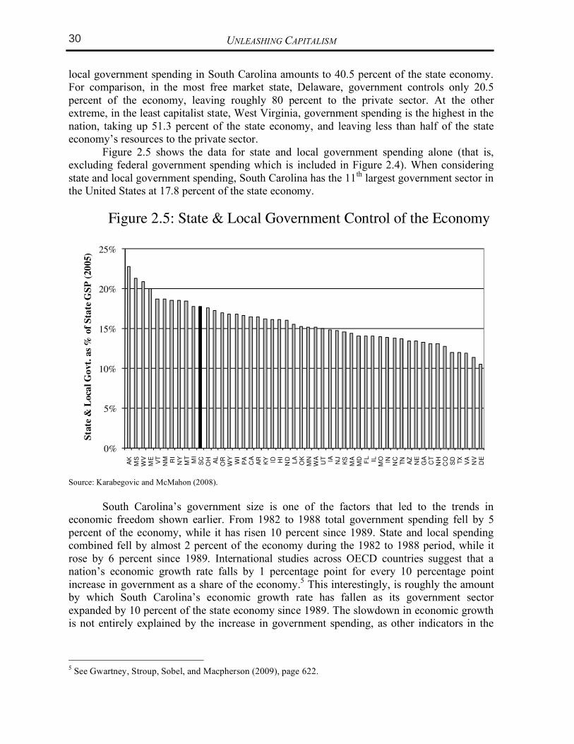
UNLEASHING CAPITALISM
local government spending in South Carolina amounts to 40.5 percent of the state economy. For comparison, in the most free market state, Delaware, government controls only 20.5 percent of the economy, leaving roughly 80 percent to the private sector. At the other extreme, in the least capitalist state, West Virginia, government spending is the highest in the nation, taking up 51.3 percent of the state economy, and leaving less than half of the state economy’s resources to the private sector.
Figure 2.5 shows the data for state and local government spending alone (that is, excluding federal government spending which is included in Figure 2.4). When considering state and local government spending, South Carolina has the 11th largest government sector in the United States at 17.8 percent of the state economy.
Figure 2.5: State & Local Government Control of the Economy
0%
5%
10%
15%
20%
25%
Source: Karabegovic and McMahon (2008).
South Carolina’s government size is one of the factors that led to the trends in
economic freedom shown earlier. From 1982 to 1988 total government spending fell by 5 percent of the economy, while it has risen 10 percent since 1989. State and local spending combined fell by almost 2 percent of the economy during the 1982 to 1988 period, while it rose by 6 percent since 1989. International studies across OECD countries suggest that a nation’s economic growth rate falls by 1 percentage point for every 10 percentage point increase in government as a share of the economy.5 This interestingly, is roughly the amount by which South Carolina’s economic growth rate has fallen as its government sector expanded by 10 percent of the state economy since 1989. The slowdown in economic growth is not entirely explained by the increase in government spending, as other indicators in the
5 See Gwartney, Stroup, Sobel, and Macpherson (2009), page 622.
CHAPTER 2: THE SOURCES OF ECONOMIC GROWTH
economic freedom index show similar trends. South Carolina’s scores on nine of the ten index components rose from 1982 to 1988, while 8 of the 10 fell in the subsequent decade.6
DID HURRICANE HUGO PLAY A ROLE?
Astute readers may notice that South Carolina’s first downward trend began around 1989, the year in which Hurricane Hugo hit South Carolina, causing roughly $6 billion in damage to the state, and resulting in 24 of South Carolina’s 46 counties being declared disaster areas.7 At the time Hurricane Hugo was the costliest hurricane in U.S. history, although it has now been surpassed by four other hurricanes, including Hurricanes Andrew and Katrina. With regard to economic prosperity, evidence from states like South Carolina, as well as Florida and North Carolina who also suffer from regular hurricane strikes, suggests that a state recovers fairly quickly. South Carolina’s ranking in per capita income, for example, had returned to its 1988 level by the mid-1990s. Louisiana, after falling to 50th in per capita income after Hurricane Katrina struck, has already rebounded and is now ranked higher than it was prior to the storm in per capita income, although conditions there may be different from the post-Hugo situation as there was a much larger permanent outflow of low-income population from Louisiana due to the storm. While economic activity was eventually restored, the lasting negative impact of Hurricane Hugo is likely found mostly in its impact on economic freedom—especially the size of government—in South Carolina. Higgs (1987) notes that throughout the history of the United States, individual ‘crisis’ events are often met with supposedly temporary increases in government spending or programs that often persist forever. One need only think of the many new federal programs enacted after the September 11th terrorist attacks as an example of this process. Therefore, events such as Hurricane Hugo often lead to permanent ‘ratchets’ upward in government spending, regulations, and other market interventions (such as price controls and regulations).
In addition, research by Leeson and Sobel (2008) shows that the massive inflows of federal FEMA spending that accompany hurricanes tend to result in increases in state government corruption, bureaucracy, and increases in special interest group influence in state government in a manner similar to what unfolds accompanying large inflows of foreign aid to poorer countries in the world. After Hurricane Hugo, FEMA rapidly injected over $387 million of federal spending into South Carolina. For comparison, this would be roughly 0.6 percent of the state economy at the time, 5.6 percent of South Carolina state government spending that year, or $112 per person in the state. South Carolina’s economic freedom has shown a mostly downward trend since Hurricane Hugo, and if this storm is to be blamed for anything, it would be its lasting deterioration of the economic freedoms South Carolinians enjoyed prior to the storm’s landfall in Charleston on the night of September 21, 1989.
6 These 10 index components measure a variety of factors including government spending, taxes, regulations,
and the security of property rights. 7 See Guimaraes, Hefner, and Woodward (1993).
UNLEASHING CAPITALISM
local government spending in South Carolina amounts to 40.5 percent of the state economy. For comparison, in the most free market state, Delaware, government controls only 20.5 percent of the economy, leaving roughly 80 percent to the private sector. At the other extreme, in the least capitalist state, West Virginia, government spending is the highest in the nation, taking up 51.3 percent of the state economy, and leaving less than half of the state economy’s resources to the private sector.
Figure 2.5 shows the data for state and local government spending alone (that is, excluding federal government spending which is included in Figure 2.4). When considering state and local government spending, South Carolina has the 11th largest government sector in the United States at 17.8 percent of the state economy.
Figure 2.5: State & Local Government Control of the Economy
0%
5%
10%
15%
20%
25%
AK
MS
WV
MEVT
NM RI
NY
MT
MI
SC
OH AL
OR
WY
WI
PA
CA
AR
KY ID HI
ND LA
OK
MN
WA
UT IA NJ
KS
MA
MD FL IL
MO IN NC
TNAZ
NE
GA
CT
NH
CO
SD TX
VA
NV
DE
Sta
te &
Loca
l G
ovt.
as
% o
f S
tate
GS
P (
20
05)
Source: Karabegovic and McMahon (2008).
South Carolina’s government size is one of the factors that led to the trends in
economic freedom shown earlier. From 1982 to 1988 total government spending fell by 5 percent of the economy, while it has risen 10 percent since 1989. State and local spending combined fell by almost 2 percent of the economy during the 1982 to 1988 period, while it rose by 6 percent since 1989. International studies across OECD countries suggest that a nation’s economic growth rate falls by 1 percentage point for every 10 percentage point increase in government as a share of the economy.5 This interestingly, is roughly the amount by which South Carolina’s economic growth rate has fallen as its government sector expanded by 10 percent of the state economy since 1989. The slowdown in economic growth is not entirely explained by the increase in government spending, as other indicators in the
5 See Gwartney, Stroup, Sobel, and Macpherson (2009), page 622.
UNLEASHING CAPITALISM 18
manufacturing property tax in the country. In Figure 5.8 we present the effective property tax rates data for Southeastern states, for comparison. The ranks given for the states are out of all 50 states. The ‘net tax’ and ‘effective tax rate’ are calculated based on property valued at $25 million ($12.5 million in machinery and equipment, $12.5 million in inventories, and $2.5 million in fixtures). Notice that South Carolina’s effective tax rate on industrial property is over 7.8 times higher than the most industry-friendly state, Delaware. (Delaware is listed in the figure because it is the lowest-tax state.)
Figure 5.8: Industrial Property Taxes in Southeastern states*, 2007 State Rank (of 50) Net Tax Effective Tax Rate
South Carolina 1 $1,864,900 3.73%
Mississippi 4 $1,291,050 2.58%
Texas 6 $1,264,358 2.53%
Tennessee 10 $1,033,544 2.07%
West Virginia 14 $833,234 1.67%
Louisiana 17 $783,407 1.57%
Georgia 20 $760,381 1.52%
Florida 24 $677,683 1.36%
Alabama 35 $533,776 1.11%
North Carolina 37 $491,071 0.98%
Kentucky 47 $327,100 0.65%
Virginia 49 $241,498 0.48%
Delaware 50 $238,840 0.48%
Source: National Association of Manufacturers (2009) * Taxes measured in the states’ largest city only.
Importantly, South Carolina’s effective tax rate is almost 2.5 times greater than Georgia’s tax, and almost 4 times greater than North Carolina’s. This puts South Carolina at a serious disadvantage, in terms of its ability to attract and keep industry. Since South Carolina has the highest tax in the country on industrial property, it should be no surprise that it has one of the lowest per capita incomes and economic growth rates in the country. Although it is probably not critical that South Carolina set its tax rate to the lowest in the country, it should definitely make it at least competitive for the Southeast. Since Georgia’s rate is effectively 1.52 percent and North Carolina’s is just under 1 percent, a rate at around 1 percent might be sufficient to attract more industry. Working to reduce the various taxes applied to industry would seriously improve the state’s competitiveness. Such a significant reduction in taxes on industrial property would obviously lead to a reduction in tax revenues on industrial property, at least initially. However, the overall revenue may in fact increase once the growth rate in the state begins to pick up and more industry moves into the state. Furthermore, if the official tax rates are lowered, then the state
30 CHAPTER 5: SPECIFIC TAX REFORMS
13
Presumably the original intent of imposing a tax rate schedule with graduated marginal tax rates was to make the income tax progressive. However, what progressivity exists in the state’s income tax structure is due to the zero tax on the first $2,630 of income, and because of the graduated marginal tax rates. However, since the marginal tax rate increases over such small steps in income, as shown in Figure 5.5, most of the progressivity occurs at lower income levels, not higher levels of income. At higher income levels, the average tax rate hardly increases at all. This nature of the current tax is directly contradictory to the goal of progressivity. So although on the surface it appears that the tax satisfies the vertical equity condition, it really does this only at the lower income levels reducing the wealth of these lowest income taxpayers, not the intended consequence.
Figure 5.5: South Carolina income tax: Current tax rates compared to inflation-indexed rates, 2009
Current Income Tax
Rates/Brackets
Income Tax Rates/Brackets if 1959 Tax Schedule was Inflation Adjusted to
2009
Taxable Income Tax
Amount Average Tax Rate
Tax Amount
Average Tax Rate
$5,000 $71 1.42% $125 2.5%
$10,000 $290 2.90% $250 2.5%
$15,000 $604 4.03% $377 2.51%
$20,000 $954 4.77% $527 2.63%
$30,000 $1,654 5.51% $834 2.78%
$50,000 $3,054 6.10% $1,695 3.39%
$75,000 $4,804 6.41% $3,127 4.17%
$100,000 $6,554 6.56% $4,877 4.88%
$150,000 $10,054 6.70% $8,377 5.58%
$200,000 $13,554 6.77% $11,877 5.94%
Figure 5.5 also shows what the average tax rates are for various incomes and taxes
under the current tax system in South Carolina. In the right columns it also shows what the taxes and average tax rates would be if the 1959 tax tables were indexed for inflation. The figure clearly shows that the 1959 indexed tax rate structure is more uniformly progressive, especially at higher levels of incomes. It keeps tax rates extremely low for the lowest income individuals in the state. Figure 5.5 also shows that the current tax system charges all income groups more in taxes than an indexed rate schedule. The only exception is the $5,000 income earner in the table. As South Carolina income taxes continue to climb while the tax brackets remain stagnant, the state becomes a relatively high-tax state. This has a negative impact on
UNLEASHING CAPITALISM
local government spending in South Carolina amounts to 40.5 percent of the state economy. For comparison, in the most free market state, Delaware, government controls only 20.5 percent of the economy, leaving roughly 80 percent to the private sector. At the other extreme, in the least capitalist state, West Virginia, government spending is the highest in the nation, taking up 51.3 percent of the state economy, and leaving less than half of the state economy’s resources to the private sector.
Figure 2.5 shows the data for state and local government spending alone (that is, excluding federal government spending which is included in Figure 2.4). When considering state and local government spending, South Carolina has the 11th largest government sector in the United States at 17.8 percent of the state economy.
Figure 2.5: State & Local Government Control of the Economy
0%
5%
10%
15%
20%
25%
Source: Karabegovic and McMahon (2008).
South Carolina’s government size is one of the factors that led to the trends in
economic freedom shown earlier. From 1982 to 1988 total government spending fell by 5 percent of the economy, while it has risen 10 percent since 1989. State and local spending combined fell by almost 2 percent of the economy during the 1982 to 1988 period, while it rose by 6 percent since 1989. International studies across OECD countries suggest that a nation’s economic growth rate falls by 1 percentage point for every 10 percentage point increase in government as a share of the economy.5 This interestingly, is roughly the amount by which South Carolina’s economic growth rate has fallen as its government sector expanded by 10 percent of the state economy since 1989. The slowdown in economic growth is not entirely explained by the increase in government spending, as other indicators in the
5 See Gwartney, Stroup, Sobel, and Macpherson (2009), page 622.
CHAPTER 2: THE SOURCES OF ECONOMIC GROWTH
economic freedom index show similar trends. South Carolina’s scores on nine of the ten index components rose from 1982 to 1988, while 8 of the 10 fell in the subsequent decade.6
DID HURRICANE HUGO PLAY A ROLE?
Astute readers may notice that South Carolina’s first downward trend began around 1989, the year in which Hurricane Hugo hit South Carolina, causing roughly $6 billion in damage to the state, and resulting in 24 of South Carolina’s 46 counties being declared disaster areas.7 At the time Hurricane Hugo was the costliest hurricane in U.S. history, although it has now been surpassed by four other hurricanes, including Hurricanes Andrew and Katrina. With regard to economic prosperity, evidence from states like South Carolina, as well as Florida and North Carolina who also suffer from regular hurricane strikes, suggests that a state recovers fairly quickly. South Carolina’s ranking in per capita income, for example, had returned to its 1988 level by the mid-1990s. Louisiana, after falling to 50th in per capita income after Hurricane Katrina struck, has already rebounded and is now ranked higher than it was prior to the storm in per capita income, although conditions there may be different from the post-Hugo situation as there was a much larger permanent outflow of low-income population from Louisiana due to the storm. While economic activity was eventually restored, the lasting negative impact of Hurricane Hugo is likely found mostly in its impact on economic freedom—especially the size of government—in South Carolina. Higgs (1987) notes that throughout the history of the United States, individual ‘crisis’ events are often met with supposedly temporary increases in government spending or programs that often persist forever. One need only think of the many new federal programs enacted after the September 11th terrorist attacks as an example of this process. Therefore, events such as Hurricane Hugo often lead to permanent ‘ratchets’ upward in government spending, regulations, and other market interventions (such as price controls and regulations).
In addition, research by Leeson and Sobel (2008) shows that the massive inflows of federal FEMA spending that accompany hurricanes tend to result in increases in state government corruption, bureaucracy, and increases in special interest group influence in state government in a manner similar to what unfolds accompanying large inflows of foreign aid to poorer countries in the world. After Hurricane Hugo, FEMA rapidly injected over $387 million of federal spending into South Carolina. For comparison, this would be roughly 0.6 percent of the state economy at the time, 5.6 percent of South Carolina state government spending that year, or $112 per person in the state. South Carolina’s economic freedom has shown a mostly downward trend since Hurricane Hugo, and if this storm is to be blamed for anything, it would be its lasting deterioration of the economic freedoms South Carolinians enjoyed prior to the storm’s landfall in Charleston on the night of September 21, 1989.
6 These 10 index components measure a variety of factors including government spending, taxes, regulations,
and the security of property rights. 7 See Guimaraes, Hefner, and Woodward (1993).
UNLEASHING CAPITALISM 18
manufacturing property tax in the country. In Figure 5.8 we present the effective property tax rates data for Southeastern states, for comparison. The ranks given for the states are out of all 50 states. The ‘net tax’ and ‘effective tax rate’ are calculated based on property valued at $25 million ($12.5 million in machinery and equipment, $12.5 million in inventories, and $2.5 million in fixtures). Notice that South Carolina’s effective tax rate on industrial property is over 7.8 times higher than the most industry-friendly state, Delaware. (Delaware is listed in the figure because it is the lowest-tax state.)
Figure 5.8: Industrial Property Taxes in Southeastern states*, 2007 State Rank (of 50) Net Tax Effective Tax Rate
South Carolina 1 $1,864,900 3.73%
Mississippi 4 $1,291,050 2.58%
Texas 6 $1,264,358 2.53%
Tennessee 10 $1,033,544 2.07%
West Virginia 14 $833,234 1.67%
Louisiana 17 $783,407 1.57%
Georgia 20 $760,381 1.52%
Florida 24 $677,683 1.36%
Alabama 35 $533,776 1.11%
North Carolina 37 $491,071 0.98%
Kentucky 47 $327,100 0.65%
Virginia 49 $241,498 0.48%
Delaware 50 $238,840 0.48%
Source: National Association of Manufacturers (2009) * Taxes measured in the states’ largest city only.
Importantly, South Carolina’s effective tax rate is almost 2.5 times greater than Georgia’s tax, and almost 4 times greater than North Carolina’s. This puts South Carolina at a serious disadvantage, in terms of its ability to attract and keep industry. Since South Carolina has the highest tax in the country on industrial property, it should be no surprise that it has one of the lowest per capita incomes and economic growth rates in the country. Although it is probably not critical that South Carolina set its tax rate to the lowest in the country, it should definitely make it at least competitive for the Southeast. Since Georgia’s rate is effectively 1.52 percent and North Carolina’s is just under 1 percent, a rate at around 1 percent might be sufficient to attract more industry. Working to reduce the various taxes applied to industry would seriously improve the state’s competitiveness. Such a significant reduction in taxes on industrial property would obviously lead to a reduction in tax revenues on industrial property, at least initially. However, the overall revenue may in fact increase once the growth rate in the state begins to pick up and more industry moves into the state. Furthermore, if the official tax rates are lowered, then the state
31CHAPTER 5: SPECIFIC TAX REFORMS
13
Presumably the original intent of imposing a tax rate schedule with graduated marginal tax rates was to make the income tax progressive. However, what progressivity exists in the state’s income tax structure is due to the zero tax on the first $2,630 of income, and because of the graduated marginal tax rates. However, since the marginal tax rate increases over such small steps in income, as shown in Figure 5.5, most of the progressivity occurs at lower income levels, not higher levels of income. At higher income levels, the average tax rate hardly increases at all. This nature of the current tax is directly contradictory to the goal of progressivity. So although on the surface it appears that the tax satisfies the vertical equity condition, it really does this only at the lower income levels reducing the wealth of these lowest income taxpayers, not the intended consequence.
Figure 5.5: South Carolina income tax: Current tax rates compared to inflation-indexed rates, 2009
Current Income Tax
Rates/Brackets
Income Tax Rates/Brackets if 1959 Tax Schedule was Inflation Adjusted to
2009
Taxable Income Tax
Amount Average Tax Rate
Tax Amount
Average Tax Rate
$5,000 $71 1.42% $125 2.5%
$10,000 $290 2.90% $250 2.5%
$15,000 $604 4.03% $377 2.51%
$20,000 $954 4.77% $527 2.63%
$30,000 $1,654 5.51% $834 2.78%
$50,000 $3,054 6.10% $1,695 3.39%
$75,000 $4,804 6.41% $3,127 4.17%
$100,000 $6,554 6.56% $4,877 4.88%
$150,000 $10,054 6.70% $8,377 5.58%
$200,000 $13,554 6.77% $11,877 5.94%
Figure 5.5 also shows what the average tax rates are for various incomes and taxes
under the current tax system in South Carolina. In the right columns it also shows what the taxes and average tax rates would be if the 1959 tax tables were indexed for inflation. The figure clearly shows that the 1959 indexed tax rate structure is more uniformly progressive, especially at higher levels of incomes. It keeps tax rates extremely low for the lowest income individuals in the state. Figure 5.5 also shows that the current tax system charges all income groups more in taxes than an indexed rate schedule. The only exception is the $5,000 income earner in the table. As South Carolina income taxes continue to climb while the tax brackets remain stagnant, the state becomes a relatively high-tax state. This has a negative impact on
UNLEASHING CAPITALISM
SOUTH CAROLINA’S OTHER ECONOMIC POLICY RANKINGS
Not only does South Carolina’s economic freedom ranking show the need for policy reform, but nearly every other national index of business climate agrees. Below are South Carolina’s most recent rankings in all of the major national indices of business climate related issues.8 South Carolina’s Business Climate Rankings:
7th Small Business & Entrepreneurship Council’s Small Business Survival Index (2008) 11th Small Business & Entrepreneurship Council’s Small Business Tax Index (2009)
25th Tax Foundation’s State Business Tax Climate Index (2009)
25th Fraser Institute’s Economic Freedom of North America (2005) 27th Directorship Magazine’s Boardroom Guide to the Best States for Business (2009)
37th CNBC’s America’s Top States for Business (2009)
40th Corporation for Enterprise Development’s (CFED) Development Capacity Index (2007)
41st Progressive Policy Institute’s (PPI) New Economy Index (2002) 42nd Beacon Hill Institute’s State Competitiveness Report (2007)
42nd Milken Institute’s National State Technology & Science Index (2008)
43rd Institute for Legal Reform (ILR) / Harris State Liability Systems Ranking Study (2008) 45th Milken Institute’s Cost of Doing Business Index (2007)
Beside the two small business rankings from the Small Business & Entrepreneurship
Council, South Carolina generally ranks in the 30s or 40s in most others. These indices are to one extent or another measuring the same thing; South Carolina’s lack of reliance on capitalism. Even South Carolina’s individual income tax is among the worse in the nation, with a six bracket tax code that is virtually identical to what it was in 1959 when median family income was $3,821 and the top, 7 percent, tax bracket began at $10,000. At that time the median family was in the second lowest, or 3 percent, tax bracket. Because of a failure to update the brackets properly through time for inflation South Carolina’s top 7 percent tax bracket started at $13,350 in 2008, meaning the vast majority of families have now been artificially moved into the highest tax bracket because of inflation. For comparison, the 2007 median family income in South Carolina was $52,913. Had the 1959 tax brackets been properly updated for inflation, the top 7 percent bracket would not begin until an income level of $73,987 in 2008, and the median family would be in the third lowest, or 4 percent, tax bracket. This would be more similar to other states like North Carolina whose 7.75 percent top rate begins at $60,000 or West Virginia whose 6.5 percent top rate also begins at $60,000.
Essentially, South Carolina now has an individual income tax system that is almost a flat rate system in which virtually all taxpayers in the state are in one bracket. The difference is that the other states with flat rate systems have significantly lower rates, with Illinois at 3 percent, Pennsylvania at 3.07 percent, Indiana at 3.4 percent, Michigan at 4.35 percent,
8 These rankings can be found online at the following websites, http://www.milkeninstitute.org (two),
http://www.taxfoundation.org, http://www.neweconomyindex.org/, http://www.beaconhill.org,
http://www.sbecouncil.org (two), http://www.cfed.org, http://www.instituteforlegalreform.com,
http://www.directorship.com, http://www.cnbc.com, http://www.freetheworld.com.
CHAPTER 2: THE SOURCES OF ECONOMIC GROWTH
Colorado at 4.63 percent, and Massachusetts at 5.3 percent. Thus, South Carolina imposes a marginal income tax rate on its median family almost twice as high as these other states.
In addition to South Carolina’s uncompetitive individual income tax rates, the effective property tax rate on industrial property in the state is the highest in the nation. A study by the Minnesota Center for Public Finance Research that appears in the 2009 Competitiveness Redbook published by the National Association of Manufacturers provides a ranking of the tax burden on a representative manufacturing business with $25 million of property consisting of $12.5 million in machinery and equipment, $10 million in inventories, and $2.5 million in fixtures. South Carolina ranks first, with an annual property tax bill of $1,864,900 which amounts to a 3.73 percent effective tax rate. For comparison, in the most free market state, Delaware, this same business’s property tax bill would be $238,840 (an effective rate of 0.478 percent, the lowest in the nation). Thus, the annual property tax bill for an identical manufacturing business in Delaware is about 13 percent of the tax bill they face in South Carolina.
Perhaps more importantly, the property taxes levied on this business would be $760,381 in Georgia, and $491,071 in North Carolina. With effective tax rates of 1.521 percent and 0.982 percent respectively, the property tax this representative firm would face in South Carolina’s neighboring states is only a fraction of what it is in South Carolina (41 percent for Georgia and 26 percent for North Carolina). The high property tax rates South Carolina imposes on equipment and machinery result in less capital investment and reduced prosperity for all South Carolinians.
We will return specifically to the issue of South Carolina’s taxes, and potential areas for reform, in Chapters 4 and 5.
SOUTH CAROLINA HAS LOW ECONOMIC FREEDOM RELATIVE TO
ITS NEIGHBORING STATES
South Carolina’s lack of economic freedom, especially relative to its neighboring states, is drawing business out of the state. While South Carolina ranked 25th in economic freedom in 2005, Georgia and North Carolina both ranked in the top 5—in fact, they were tied for third with Colorado. Only Texas and Delaware ranked higher in economic freedom than South Carolina’s two neighboring states.
Georgia and North Carolina also both ranked in the top 10 of CNBC’s America’s Top States for Business, while South Carolina ranked 37th. In fact, South Carolina ranks lower than both of its neighboring states in 9 out of the 12 business climate rankings presented earlier in this chapter. Because business location decisions are most flexible across neighboring state lines, this is problematic for South Carolina. It also increases the importance of making policy reforms in the Palmetto State an immediate priority.
Because of their better business climates, Georgia and North Carolina have created a more vibrant entrepreneurial environment. Measures of entrepreneurial activity, including venture capital investments per capita, patents per capita, establishment birth rates for large firms, and the growth rate of sole proprietorships, show South Carolina lagging behind its neighboring states.9
9 See Figure 2.7 for the actual numbers.
UNLEASHING CAPITALISM 18
manufacturing property tax in the country. In Figure 5.8 we present the effective property tax rates data for Southeastern states, for comparison. The ranks given for the states are out of all 50 states. The ‘net tax’ and ‘effective tax rate’ are calculated based on property valued at $25 million ($12.5 million in machinery and equipment, $12.5 million in inventories, and $2.5 million in fixtures). Notice that South Carolina’s effective tax rate on industrial property is over 7.8 times higher than the most industry-friendly state, Delaware. (Delaware is listed in the figure because it is the lowest-tax state.)
Figure 5.8: Industrial Property Taxes in Southeastern states*, 2007 State Rank (of 50) Net Tax Effective Tax Rate
South Carolina 1 $1,864,900 3.73%
Mississippi 4 $1,291,050 2.58%
Texas 6 $1,264,358 2.53%
Tennessee 10 $1,033,544 2.07%
West Virginia 14 $833,234 1.67%
Louisiana 17 $783,407 1.57%
Georgia 20 $760,381 1.52%
Florida 24 $677,683 1.36%
Alabama 35 $533,776 1.11%
North Carolina 37 $491,071 0.98%
Kentucky 47 $327,100 0.65%
Virginia 49 $241,498 0.48%
Delaware 50 $238,840 0.48%
Source: National Association of Manufacturers (2009) * Taxes measured in the states’ largest city only.
Importantly, South Carolina’s effective tax rate is almost 2.5 times greater than Georgia’s tax, and almost 4 times greater than North Carolina’s. This puts South Carolina at a serious disadvantage, in terms of its ability to attract and keep industry. Since South Carolina has the highest tax in the country on industrial property, it should be no surprise that it has one of the lowest per capita incomes and economic growth rates in the country. Although it is probably not critical that South Carolina set its tax rate to the lowest in the country, it should definitely make it at least competitive for the Southeast. Since Georgia’s rate is effectively 1.52 percent and North Carolina’s is just under 1 percent, a rate at around 1 percent might be sufficient to attract more industry. Working to reduce the various taxes applied to industry would seriously improve the state’s competitiveness. Such a significant reduction in taxes on industrial property would obviously lead to a reduction in tax revenues on industrial property, at least initially. However, the overall revenue may in fact increase once the growth rate in the state begins to pick up and more industry moves into the state. Furthermore, if the official tax rates are lowered, then the state
32 CHAPTER 5: SPECIFIC TAX REFORMS
13
Presumably the original intent of imposing a tax rate schedule with graduated marginal tax rates was to make the income tax progressive. However, what progressivity exists in the state’s income tax structure is due to the zero tax on the first $2,630 of income, and because of the graduated marginal tax rates. However, since the marginal tax rate increases over such small steps in income, as shown in Figure 5.5, most of the progressivity occurs at lower income levels, not higher levels of income. At higher income levels, the average tax rate hardly increases at all. This nature of the current tax is directly contradictory to the goal of progressivity. So although on the surface it appears that the tax satisfies the vertical equity condition, it really does this only at the lower income levels reducing the wealth of these lowest income taxpayers, not the intended consequence.
Figure 5.5: South Carolina income tax: Current tax rates compared to inflation-indexed rates, 2009
Current Income Tax
Rates/Brackets
Income Tax Rates/Brackets if 1959 Tax Schedule was Inflation Adjusted to
2009
Taxable Income Tax
Amount Average Tax Rate
Tax Amount
Average Tax Rate
$5,000 $71 1.42% $125 2.5%
$10,000 $290 2.90% $250 2.5%
$15,000 $604 4.03% $377 2.51%
$20,000 $954 4.77% $527 2.63%
$30,000 $1,654 5.51% $834 2.78%
$50,000 $3,054 6.10% $1,695 3.39%
$75,000 $4,804 6.41% $3,127 4.17%
$100,000 $6,554 6.56% $4,877 4.88%
$150,000 $10,054 6.70% $8,377 5.58%
$200,000 $13,554 6.77% $11,877 5.94%
Figure 5.5 also shows what the average tax rates are for various incomes and taxes
under the current tax system in South Carolina. In the right columns it also shows what the taxes and average tax rates would be if the 1959 tax tables were indexed for inflation. The figure clearly shows that the 1959 indexed tax rate structure is more uniformly progressive, especially at higher levels of incomes. It keeps tax rates extremely low for the lowest income individuals in the state. Figure 5.5 also shows that the current tax system charges all income groups more in taxes than an indexed rate schedule. The only exception is the $5,000 income earner in the table. As South Carolina income taxes continue to climb while the tax brackets remain stagnant, the state becomes a relatively high-tax state. This has a negative impact on
UNLEASHING CAPITALISM
SOUTH CAROLINA’S OTHER ECONOMIC POLICY RANKINGS
Not only does South Carolina’s economic freedom ranking show the need for policy reform, but nearly every other national index of business climate agrees. Below are South Carolina’s most recent rankings in all of the major national indices of business climate related issues.8 South Carolina’s Business Climate Rankings:
7th Small Business & Entrepreneurship Council’s Small Business Survival Index (2008) 11th Small Business & Entrepreneurship Council’s Small Business Tax Index (2009)
25th Tax Foundation’s State Business Tax Climate Index (2009)
25th Fraser Institute’s Economic Freedom of North America (2005) 27th Directorship Magazine’s Boardroom Guide to the Best States for Business (2009)
37th CNBC’s America’s Top States for Business (2009)
40th Corporation for Enterprise Development’s (CFED) Development Capacity Index (2007)
41st Progressive Policy Institute’s (PPI) New Economy Index (2002) 42nd Beacon Hill Institute’s State Competitiveness Report (2007)
42nd Milken Institute’s National State Technology & Science Index (2008)
43rd Institute for Legal Reform (ILR) / Harris State Liability Systems Ranking Study (2008) 45th Milken Institute’s Cost of Doing Business Index (2007)
Beside the two small business rankings from the Small Business & Entrepreneurship
Council, South Carolina generally ranks in the 30s or 40s in most others. These indices are to one extent or another measuring the same thing; South Carolina’s lack of reliance on capitalism. Even South Carolina’s individual income tax is among the worse in the nation, with a six bracket tax code that is virtually identical to what it was in 1959 when median family income was $3,821 and the top, 7 percent, tax bracket began at $10,000. At that time the median family was in the second lowest, or 3 percent, tax bracket. Because of a failure to update the brackets properly through time for inflation South Carolina’s top 7 percent tax bracket started at $13,350 in 2008, meaning the vast majority of families have now been artificially moved into the highest tax bracket because of inflation. For comparison, the 2007 median family income in South Carolina was $52,913. Had the 1959 tax brackets been properly updated for inflation, the top 7 percent bracket would not begin until an income level of $73,987 in 2008, and the median family would be in the third lowest, or 4 percent, tax bracket. This would be more similar to other states like North Carolina whose 7.75 percent top rate begins at $60,000 or West Virginia whose 6.5 percent top rate also begins at $60,000.
Essentially, South Carolina now has an individual income tax system that is almost a flat rate system in which virtually all taxpayers in the state are in one bracket. The difference is that the other states with flat rate systems have significantly lower rates, with Illinois at 3 percent, Pennsylvania at 3.07 percent, Indiana at 3.4 percent, Michigan at 4.35 percent,
8 These rankings can be found online at the following websites, http://www.milkeninstitute.org (two),
http://www.taxfoundation.org, http://www.neweconomyindex.org/, http://www.beaconhill.org,
http://www.sbecouncil.org (two), http://www.cfed.org, http://www.instituteforlegalreform.com,
http://www.directorship.com, http://www.cnbc.com, http://www.freetheworld.com.
CHAPTER 2: THE SOURCES OF ECONOMIC GROWTH
Colorado at 4.63 percent, and Massachusetts at 5.3 percent. Thus, South Carolina imposes a marginal income tax rate on its median family almost twice as high as these other states.
In addition to South Carolina’s uncompetitive individual income tax rates, the effective property tax rate on industrial property in the state is the highest in the nation. A study by the Minnesota Center for Public Finance Research that appears in the 2009 Competitiveness Redbook published by the National Association of Manufacturers provides a ranking of the tax burden on a representative manufacturing business with $25 million of property consisting of $12.5 million in machinery and equipment, $10 million in inventories, and $2.5 million in fixtures. South Carolina ranks first, with an annual property tax bill of $1,864,900 which amounts to a 3.73 percent effective tax rate. For comparison, in the most free market state, Delaware, this same business’s property tax bill would be $238,840 (an effective rate of 0.478 percent, the lowest in the nation). Thus, the annual property tax bill for an identical manufacturing business in Delaware is about 13 percent of the tax bill they face in South Carolina.
Perhaps more importantly, the property taxes levied on this business would be $760,381 in Georgia, and $491,071 in North Carolina. With effective tax rates of 1.521 percent and 0.982 percent respectively, the property tax this representative firm would face in South Carolina’s neighboring states is only a fraction of what it is in South Carolina (41 percent for Georgia and 26 percent for North Carolina). The high property tax rates South Carolina imposes on equipment and machinery result in less capital investment and reduced prosperity for all South Carolinians.
We will return specifically to the issue of South Carolina’s taxes, and potential areas for reform, in Chapters 4 and 5.
SOUTH CAROLINA HAS LOW ECONOMIC FREEDOM RELATIVE TO
ITS NEIGHBORING STATES
South Carolina’s lack of economic freedom, especially relative to its neighboring states, is drawing business out of the state. While South Carolina ranked 25th in economic freedom in 2005, Georgia and North Carolina both ranked in the top 5—in fact, they were tied for third with Colorado. Only Texas and Delaware ranked higher in economic freedom than South Carolina’s two neighboring states.
Georgia and North Carolina also both ranked in the top 10 of CNBC’s America’s Top States for Business, while South Carolina ranked 37th. In fact, South Carolina ranks lower than both of its neighboring states in 9 out of the 12 business climate rankings presented earlier in this chapter. Because business location decisions are most flexible across neighboring state lines, this is problematic for South Carolina. It also increases the importance of making policy reforms in the Palmetto State an immediate priority.
Because of their better business climates, Georgia and North Carolina have created a more vibrant entrepreneurial environment. Measures of entrepreneurial activity, including venture capital investments per capita, patents per capita, establishment birth rates for large firms, and the growth rate of sole proprietorships, show South Carolina lagging behind its neighboring states.9
9 See Figure 2.7 for the actual numbers.
UNLEASHING CAPITALISM 18
manufacturing property tax in the country. In Figure 5.8 we present the effective property tax rates data for Southeastern states, for comparison. The ranks given for the states are out of all 50 states. The ‘net tax’ and ‘effective tax rate’ are calculated based on property valued at $25 million ($12.5 million in machinery and equipment, $12.5 million in inventories, and $2.5 million in fixtures). Notice that South Carolina’s effective tax rate on industrial property is over 7.8 times higher than the most industry-friendly state, Delaware. (Delaware is listed in the figure because it is the lowest-tax state.)
Figure 5.8: Industrial Property Taxes in Southeastern states*, 2007 State Rank (of 50) Net Tax Effective Tax Rate
South Carolina 1 $1,864,900 3.73%
Mississippi 4 $1,291,050 2.58%
Texas 6 $1,264,358 2.53%
Tennessee 10 $1,033,544 2.07%
West Virginia 14 $833,234 1.67%
Louisiana 17 $783,407 1.57%
Georgia 20 $760,381 1.52%
Florida 24 $677,683 1.36%
Alabama 35 $533,776 1.11%
North Carolina 37 $491,071 0.98%
Kentucky 47 $327,100 0.65%
Virginia 49 $241,498 0.48%
Delaware 50 $238,840 0.48%
Source: National Association of Manufacturers (2009) * Taxes measured in the states’ largest city only.
Importantly, South Carolina’s effective tax rate is almost 2.5 times greater than Georgia’s tax, and almost 4 times greater than North Carolina’s. This puts South Carolina at a serious disadvantage, in terms of its ability to attract and keep industry. Since South Carolina has the highest tax in the country on industrial property, it should be no surprise that it has one of the lowest per capita incomes and economic growth rates in the country. Although it is probably not critical that South Carolina set its tax rate to the lowest in the country, it should definitely make it at least competitive for the Southeast. Since Georgia’s rate is effectively 1.52 percent and North Carolina’s is just under 1 percent, a rate at around 1 percent might be sufficient to attract more industry. Working to reduce the various taxes applied to industry would seriously improve the state’s competitiveness. Such a significant reduction in taxes on industrial property would obviously lead to a reduction in tax revenues on industrial property, at least initially. However, the overall revenue may in fact increase once the growth rate in the state begins to pick up and more industry moves into the state. Furthermore, if the official tax rates are lowered, then the state
33CHAPTER 5: SPECIFIC TAX REFORMS
13
Presumably the original intent of imposing a tax rate schedule with graduated marginal tax rates was to make the income tax progressive. However, what progressivity exists in the state’s income tax structure is due to the zero tax on the first $2,630 of income, and because of the graduated marginal tax rates. However, since the marginal tax rate increases over such small steps in income, as shown in Figure 5.5, most of the progressivity occurs at lower income levels, not higher levels of income. At higher income levels, the average tax rate hardly increases at all. This nature of the current tax is directly contradictory to the goal of progressivity. So although on the surface it appears that the tax satisfies the vertical equity condition, it really does this only at the lower income levels reducing the wealth of these lowest income taxpayers, not the intended consequence.
Figure 5.5: South Carolina income tax: Current tax rates compared to inflation-indexed rates, 2009
Current Income Tax
Rates/Brackets
Income Tax Rates/Brackets if 1959 Tax Schedule was Inflation Adjusted to
2009
Taxable Income Tax
Amount Average Tax Rate
Tax Amount
Average Tax Rate
$5,000 $71 1.42% $125 2.5%
$10,000 $290 2.90% $250 2.5%
$15,000 $604 4.03% $377 2.51%
$20,000 $954 4.77% $527 2.63%
$30,000 $1,654 5.51% $834 2.78%
$50,000 $3,054 6.10% $1,695 3.39%
$75,000 $4,804 6.41% $3,127 4.17%
$100,000 $6,554 6.56% $4,877 4.88%
$150,000 $10,054 6.70% $8,377 5.58%
$200,000 $13,554 6.77% $11,877 5.94%
Figure 5.5 also shows what the average tax rates are for various incomes and taxes
under the current tax system in South Carolina. In the right columns it also shows what the taxes and average tax rates would be if the 1959 tax tables were indexed for inflation. The figure clearly shows that the 1959 indexed tax rate structure is more uniformly progressive, especially at higher levels of incomes. It keeps tax rates extremely low for the lowest income individuals in the state. Figure 5.5 also shows that the current tax system charges all income groups more in taxes than an indexed rate schedule. The only exception is the $5,000 income earner in the table. As South Carolina income taxes continue to climb while the tax brackets remain stagnant, the state becomes a relatively high-tax state. This has a negative impact on
UNLEASHING CAPITALISM
One of the places where this difference is visible is in the recent relative performance of the ports of Charleston and Savannah, located only about 100 miles apart.10 While container traffic at the other largest U.S. ports remained relatively constant between 2006 and 2007, Savannah’s traffic increased by almost 21 percent, allowing it to become the fourth largest port in the nation almost out of nowhere. It has been the fastest growing port in the United States since 2000; and in 2007, Savannah handled more than 2.6 million 20-foot equivalent units (TEUs) and is now home to new distribution centers for retailers like Ikea and Target. South Carolina’s weak competitive position has meant that during this same period, Charleston’s port has seen dwindling traffic. In 2005, Charleston handled 12.6 million metric tons of containerized freight including lumber, electronics and pharmaceutical products, making it the fourth largest port in the United States. By 2006, traffic had fallen by 9 percent, and then declined by another 7 percent in 2007. As a result, Charleston fell to eighth place among U.S. ports in terms of container tonnage—even behind Norfolk, Virginia. Things could get even worse in the coming years, if Maersk Line stops using the Charleston port when its contract expires in 2010.
WHAT IS CAPITALISM? THE CONCEPT OF ECONOMIC FREEDOM While everyone has a general idea of what economists mean by the term ‘capitalism’ it is important that we now define it more precisely. Fundamentally, capitalism is an economic system founded on the private ownership of the productive assets within an economy. These include land, labor (including your person), and all other tangible property (e.g., cars, houses, factories, etc.) and intangible property (e.g., radio waves, intellectual property, etc.).
Individuals are free to make decisions regarding the use of their property, with the sole constraint that they do not infringe upon the property rights of others.
The freedom of action given to private owners under a system of capitalism is why the index that ranks states and countries is called the ‘economic freedom’ index. Economic freedom is synonymous with capitalism. More specifically, the key ingredients of economic freedom and capitalism are:
� personal choice and accountability for damages to others,
� voluntary exchange, with unregulated prices negotiated by buyers and sellers,
� freedom to become an entrepreneur and compete with existing businesses, and
� protection of persons and property from physical aggression, theft, lawsuits, or confiscation by others, including the government.
The concept of capitalism is deeply rooted in the notions of individual liberty and freedom that underlie our country’s founding and are reflected in the Declaration of Independence and U.S. Constitution. Economic freedoms are based in the same philosophies that support political and civil liberties (like the freedom of speech and the freedom to elect representatives). Individuals have a right to decide how they will use their assets and talents. On the other hand, they do not have a right to the time, talents, and resources of others.
10 Data and information for this section are from Johnson (2008) and Roth (2008).
CHAPTER 2: THE SOURCES OF ECONOMIC GROWTH
Because private property rights, and their protection, are critical to economic progress, it is worthwhile to be more specific about private property rights.11 Private property rights entail three economic aspects: (1) control rights – the right to do with your property as you wish, even to exclude others from using it, so long as you do not use your property to infringe on the property rights of someone else; (2) cash flow rights – the right to the income earned from the property or its use (i.e. being the ‘residual claimant,’ which is also critical for enabling the property to be used as collateral for loans); and, (3) transferability rights – the right to sell or divest of your property under the terms and conditions you see fit.
A government policy that weakens any one of these components of property rights weakens property rights in general. Taxes, for example, restrict the cash flow rights associated with property and so weaken private property rights on that dimension.12 Regulations, on the other hand, restrict how owners may use their property, infringing on control rights, and weakening private property rights on that dimension. Outright takings, or other forms of outright expropriation, by removing the property from an owner’s possession (such as eminent domain or shoreline property takings, especially when allowing the state to remove the property from an owner’s possession and transfer it to another private owner) actually weaken property rights on all of the dimensions considered above, making property a ‘contingent right’ (contingent on the state’s arbitrary will) rather than an ‘absolute right’ guaranteed and protected by law.
In order to nurture capitalism, government must do some things but refrain from doing others. Governments promote capitalism by establishing a legal structure that provides for the even-handed enforcement of contracts and the protection of individuals and their property from aggressors seeking to use violence, coercion, and fraud to seize things that do not belong to them. However, governments must refrain from actions that weaken private property rights or interfere with personal choice, voluntary exchange, and the freedom of individuals and businesses to compete. When these government actions are substituted for personal choice, economic freedom is reduced. When government protects people and their property, enforces contracts in an unbiased manner, and provides a limited set of ‘public goods’ like roads, flood control, and other major public works projects, but leaves the rest to the private market, they support the institutions of capitalism.
11 Note that the appropriate definition of property rights are those of protective rights—that is, rights that provide
individuals with a shield against others who would invade or take what does not belong to them. Because these
are nonaggression or ‘negative’ rights, all citizens can simultaneously possess them. In the popular media some
people argue that individuals have invasive rights or what some call ‘positive rights’ to things like food, housing,
medical services, or a minimal income level. The existence of positive rights require the forceful redistribution
of wealth, which implies that some individuals have the right to use force to invade and seize the labor and
possessions of others, and such invasive rights are in conflict with economic freedom. If you can ask “at whose
expense” at the end of a statement about a claim of someone’s right, it is not—and can not be—a real right. Real
rights, such as the right to your life or free speech, do not impose further obligations on others (other than to
avoid from violating your right). The right to property does not mean you have a right to take the property of others, nor is it a guarantee you will own property—rather it is a right that protects legitimately acquired
property against the aggression from others who would take it. 12 In addition, because the value of a property asset is determined by the present discounted value of the net
income from the property’s ownership, taxes often directly impact the current market value of property to the
owners. Insecure cash flows due to taxes also inhibit long-term contracting and lending.
••••
UNLEASHING CAPITALISM 18
manufacturing property tax in the country. In Figure 5.8 we present the effective property tax rates data for Southeastern states, for comparison. The ranks given for the states are out of all 50 states. The ‘net tax’ and ‘effective tax rate’ are calculated based on property valued at $25 million ($12.5 million in machinery and equipment, $12.5 million in inventories, and $2.5 million in fixtures). Notice that South Carolina’s effective tax rate on industrial property is over 7.8 times higher than the most industry-friendly state, Delaware. (Delaware is listed in the figure because it is the lowest-tax state.)
Figure 5.8: Industrial Property Taxes in Southeastern states*, 2007 State Rank (of 50) Net Tax Effective Tax Rate
South Carolina 1 $1,864,900 3.73%
Mississippi 4 $1,291,050 2.58%
Texas 6 $1,264,358 2.53%
Tennessee 10 $1,033,544 2.07%
West Virginia 14 $833,234 1.67%
Louisiana 17 $783,407 1.57%
Georgia 20 $760,381 1.52%
Florida 24 $677,683 1.36%
Alabama 35 $533,776 1.11%
North Carolina 37 $491,071 0.98%
Kentucky 47 $327,100 0.65%
Virginia 49 $241,498 0.48%
Delaware 50 $238,840 0.48%
Source: National Association of Manufacturers (2009) * Taxes measured in the states’ largest city only.
Importantly, South Carolina’s effective tax rate is almost 2.5 times greater than Georgia’s tax, and almost 4 times greater than North Carolina’s. This puts South Carolina at a serious disadvantage, in terms of its ability to attract and keep industry. Since South Carolina has the highest tax in the country on industrial property, it should be no surprise that it has one of the lowest per capita incomes and economic growth rates in the country. Although it is probably not critical that South Carolina set its tax rate to the lowest in the country, it should definitely make it at least competitive for the Southeast. Since Georgia’s rate is effectively 1.52 percent and North Carolina’s is just under 1 percent, a rate at around 1 percent might be sufficient to attract more industry. Working to reduce the various taxes applied to industry would seriously improve the state’s competitiveness. Such a significant reduction in taxes on industrial property would obviously lead to a reduction in tax revenues on industrial property, at least initially. However, the overall revenue may in fact increase once the growth rate in the state begins to pick up and more industry moves into the state. Furthermore, if the official tax rates are lowered, then the state
34 CHAPTER 5: SPECIFIC TAX REFORMS
13
Presumably the original intent of imposing a tax rate schedule with graduated marginal tax rates was to make the income tax progressive. However, what progressivity exists in the state’s income tax structure is due to the zero tax on the first $2,630 of income, and because of the graduated marginal tax rates. However, since the marginal tax rate increases over such small steps in income, as shown in Figure 5.5, most of the progressivity occurs at lower income levels, not higher levels of income. At higher income levels, the average tax rate hardly increases at all. This nature of the current tax is directly contradictory to the goal of progressivity. So although on the surface it appears that the tax satisfies the vertical equity condition, it really does this only at the lower income levels reducing the wealth of these lowest income taxpayers, not the intended consequence.
Figure 5.5: South Carolina income tax: Current tax rates compared to inflation-indexed rates, 2009
Current Income Tax
Rates/Brackets
Income Tax Rates/Brackets if 1959 Tax Schedule was Inflation Adjusted to
2009
Taxable Income Tax
Amount Average Tax Rate
Tax Amount
Average Tax Rate
$5,000 $71 1.42% $125 2.5%
$10,000 $290 2.90% $250 2.5%
$15,000 $604 4.03% $377 2.51%
$20,000 $954 4.77% $527 2.63%
$30,000 $1,654 5.51% $834 2.78%
$50,000 $3,054 6.10% $1,695 3.39%
$75,000 $4,804 6.41% $3,127 4.17%
$100,000 $6,554 6.56% $4,877 4.88%
$150,000 $10,054 6.70% $8,377 5.58%
$200,000 $13,554 6.77% $11,877 5.94%
Figure 5.5 also shows what the average tax rates are for various incomes and taxes
under the current tax system in South Carolina. In the right columns it also shows what the taxes and average tax rates would be if the 1959 tax tables were indexed for inflation. The figure clearly shows that the 1959 indexed tax rate structure is more uniformly progressive, especially at higher levels of incomes. It keeps tax rates extremely low for the lowest income individuals in the state. Figure 5.5 also shows that the current tax system charges all income groups more in taxes than an indexed rate schedule. The only exception is the $5,000 income earner in the table. As South Carolina income taxes continue to climb while the tax brackets remain stagnant, the state becomes a relatively high-tax state. This has a negative impact on
UNLEASHING CAPITALISM
One of the places where this difference is visible is in the recent relative performance of the ports of Charleston and Savannah, located only about 100 miles apart.10 While container traffic at the other largest U.S. ports remained relatively constant between 2006 and 2007, Savannah’s traffic increased by almost 21 percent, allowing it to become the fourth largest port in the nation almost out of nowhere. It has been the fastest growing port in the United States since 2000; and in 2007, Savannah handled more than 2.6 million 20-foot equivalent units (TEUs) and is now home to new distribution centers for retailers like Ikea and Target. South Carolina’s weak competitive position has meant that during this same period, Charleston’s port has seen dwindling traffic. In 2005, Charleston handled 12.6 million metric tons of containerized freight including lumber, electronics and pharmaceutical products, making it the fourth largest port in the United States. By 2006, traffic had fallen by 9 percent, and then declined by another 7 percent in 2007. As a result, Charleston fell to eighth place among U.S. ports in terms of container tonnage—even behind Norfolk, Virginia. Things could get even worse in the coming years, if Maersk Line stops using the Charleston port when its contract expires in 2010.
WHAT IS CAPITALISM? THE CONCEPT OF ECONOMIC FREEDOM While everyone has a general idea of what economists mean by the term ‘capitalism’ it is important that we now define it more precisely. Fundamentally, capitalism is an economic system founded on the private ownership of the productive assets within an economy. These include land, labor (including your person), and all other tangible property (e.g., cars, houses, factories, etc.) and intangible property (e.g., radio waves, intellectual property, etc.).
Individuals are free to make decisions regarding the use of their property, with the sole constraint that they do not infringe upon the property rights of others.
The freedom of action given to private owners under a system of capitalism is why the index that ranks states and countries is called the ‘economic freedom’ index. Economic freedom is synonymous with capitalism. More specifically, the key ingredients of economic freedom and capitalism are:
� personal choice and accountability for damages to others,
� voluntary exchange, with unregulated prices negotiated by buyers and sellers,
� freedom to become an entrepreneur and compete with existing businesses, and
� protection of persons and property from physical aggression, theft, lawsuits, or confiscation by others, including the government.
The concept of capitalism is deeply rooted in the notions of individual liberty and freedom that underlie our country’s founding and are reflected in the Declaration of Independence and U.S. Constitution. Economic freedoms are based in the same philosophies that support political and civil liberties (like the freedom of speech and the freedom to elect representatives). Individuals have a right to decide how they will use their assets and talents. On the other hand, they do not have a right to the time, talents, and resources of others.
10 Data and information for this section are from Johnson (2008) and Roth (2008).
CHAPTER 2: THE SOURCES OF ECONOMIC GROWTH
Because private property rights, and their protection, are critical to economic progress, it is worthwhile to be more specific about private property rights.11 Private property rights entail three economic aspects: (1) control rights – the right to do with your property as you wish, even to exclude others from using it, so long as you do not use your property to infringe on the property rights of someone else; (2) cash flow rights – the right to the income earned from the property or its use (i.e. being the ‘residual claimant,’ which is also critical for enabling the property to be used as collateral for loans); and, (3) transferability rights – the right to sell or divest of your property under the terms and conditions you see fit.
A government policy that weakens any one of these components of property rights weakens property rights in general. Taxes, for example, restrict the cash flow rights associated with property and so weaken private property rights on that dimension.12 Regulations, on the other hand, restrict how owners may use their property, infringing on control rights, and weakening private property rights on that dimension. Outright takings, or other forms of outright expropriation, by removing the property from an owner’s possession (such as eminent domain or shoreline property takings, especially when allowing the state to remove the property from an owner’s possession and transfer it to another private owner) actually weaken property rights on all of the dimensions considered above, making property a ‘contingent right’ (contingent on the state’s arbitrary will) rather than an ‘absolute right’ guaranteed and protected by law.
In order to nurture capitalism, government must do some things but refrain from doing others. Governments promote capitalism by establishing a legal structure that provides for the even-handed enforcement of contracts and the protection of individuals and their property from aggressors seeking to use violence, coercion, and fraud to seize things that do not belong to them. However, governments must refrain from actions that weaken private property rights or interfere with personal choice, voluntary exchange, and the freedom of individuals and businesses to compete. When these government actions are substituted for personal choice, economic freedom is reduced. When government protects people and their property, enforces contracts in an unbiased manner, and provides a limited set of ‘public goods’ like roads, flood control, and other major public works projects, but leaves the rest to the private market, they support the institutions of capitalism.
11 Note that the appropriate definition of property rights are those of protective rights—that is, rights that provide
individuals with a shield against others who would invade or take what does not belong to them. Because these
are nonaggression or ‘negative’ rights, all citizens can simultaneously possess them. In the popular media some
people argue that individuals have invasive rights or what some call ‘positive rights’ to things like food, housing,
medical services, or a minimal income level. The existence of positive rights require the forceful redistribution
of wealth, which implies that some individuals have the right to use force to invade and seize the labor and
possessions of others, and such invasive rights are in conflict with economic freedom. If you can ask “at whose
expense” at the end of a statement about a claim of someone’s right, it is not—and can not be—a real right. Real
rights, such as the right to your life or free speech, do not impose further obligations on others (other than to
avoid from violating your right). The right to property does not mean you have a right to take the property of others, nor is it a guarantee you will own property—rather it is a right that protects legitimately acquired
property against the aggression from others who would take it. 12 In addition, because the value of a property asset is determined by the present discounted value of the net
income from the property’s ownership, taxes often directly impact the current market value of property to the
owners. Insecure cash flows due to taxes also inhibit long-term contracting and lending.
UNLEASHING CAPITALISM 18
manufacturing property tax in the country. In Figure 5.8 we present the effective property tax rates data for Southeastern states, for comparison. The ranks given for the states are out of all 50 states. The ‘net tax’ and ‘effective tax rate’ are calculated based on property valued at $25 million ($12.5 million in machinery and equipment, $12.5 million in inventories, and $2.5 million in fixtures). Notice that South Carolina’s effective tax rate on industrial property is over 7.8 times higher than the most industry-friendly state, Delaware. (Delaware is listed in the figure because it is the lowest-tax state.)
Figure 5.8: Industrial Property Taxes in Southeastern states*, 2007 State Rank (of 50) Net Tax Effective Tax Rate
South Carolina 1 $1,864,900 3.73%
Mississippi 4 $1,291,050 2.58%
Texas 6 $1,264,358 2.53%
Tennessee 10 $1,033,544 2.07%
West Virginia 14 $833,234 1.67%
Louisiana 17 $783,407 1.57%
Georgia 20 $760,381 1.52%
Florida 24 $677,683 1.36%
Alabama 35 $533,776 1.11%
North Carolina 37 $491,071 0.98%
Kentucky 47 $327,100 0.65%
Virginia 49 $241,498 0.48%
Delaware 50 $238,840 0.48%
Source: National Association of Manufacturers (2009) * Taxes measured in the states’ largest city only.
Importantly, South Carolina’s effective tax rate is almost 2.5 times greater than Georgia’s tax, and almost 4 times greater than North Carolina’s. This puts South Carolina at a serious disadvantage, in terms of its ability to attract and keep industry. Since South Carolina has the highest tax in the country on industrial property, it should be no surprise that it has one of the lowest per capita incomes and economic growth rates in the country. Although it is probably not critical that South Carolina set its tax rate to the lowest in the country, it should definitely make it at least competitive for the Southeast. Since Georgia’s rate is effectively 1.52 percent and North Carolina’s is just under 1 percent, a rate at around 1 percent might be sufficient to attract more industry. Working to reduce the various taxes applied to industry would seriously improve the state’s competitiveness. Such a significant reduction in taxes on industrial property would obviously lead to a reduction in tax revenues on industrial property, at least initially. However, the overall revenue may in fact increase once the growth rate in the state begins to pick up and more industry moves into the state. Furthermore, if the official tax rates are lowered, then the state
35CHAPTER 5: SPECIFIC TAX REFORMS
13
Presumably the original intent of imposing a tax rate schedule with graduated marginal tax rates was to make the income tax progressive. However, what progressivity exists in the state’s income tax structure is due to the zero tax on the first $2,630 of income, and because of the graduated marginal tax rates. However, since the marginal tax rate increases over such small steps in income, as shown in Figure 5.5, most of the progressivity occurs at lower income levels, not higher levels of income. At higher income levels, the average tax rate hardly increases at all. This nature of the current tax is directly contradictory to the goal of progressivity. So although on the surface it appears that the tax satisfies the vertical equity condition, it really does this only at the lower income levels reducing the wealth of these lowest income taxpayers, not the intended consequence.
Figure 5.5: South Carolina income tax: Current tax rates compared to inflation-indexed rates, 2009
Current Income Tax
Rates/Brackets
Income Tax Rates/Brackets if 1959 Tax Schedule was Inflation Adjusted to
2009
Taxable Income Tax
Amount Average Tax Rate
Tax Amount
Average Tax Rate
$5,000 $71 1.42% $125 2.5%
$10,000 $290 2.90% $250 2.5%
$15,000 $604 4.03% $377 2.51%
$20,000 $954 4.77% $527 2.63%
$30,000 $1,654 5.51% $834 2.78%
$50,000 $3,054 6.10% $1,695 3.39%
$75,000 $4,804 6.41% $3,127 4.17%
$100,000 $6,554 6.56% $4,877 4.88%
$150,000 $10,054 6.70% $8,377 5.58%
$200,000 $13,554 6.77% $11,877 5.94%
Figure 5.5 also shows what the average tax rates are for various incomes and taxes
under the current tax system in South Carolina. In the right columns it also shows what the taxes and average tax rates would be if the 1959 tax tables were indexed for inflation. The figure clearly shows that the 1959 indexed tax rate structure is more uniformly progressive, especially at higher levels of incomes. It keeps tax rates extremely low for the lowest income individuals in the state. Figure 5.5 also shows that the current tax system charges all income groups more in taxes than an indexed rate schedule. The only exception is the $5,000 income earner in the table. As South Carolina income taxes continue to climb while the tax brackets remain stagnant, the state becomes a relatively high-tax state. This has a negative impact on
UNLEASHING CAPITALISM
CAPITALISM, DEMOCRACY, AND CONSTITUTIONAL CONSTRAINTS
It is also important to distinguish between economic freedom and democracy. Unless both parties to a private exchange agree, the transaction will not occur. On the other hand, majority-rule voting is the basis for democracy. When private mutual agreement forms the basis for economic activity, there will be a strong tendency for resources to be used in ways that increase their value, creating income and wealth. The agreement of buyer and seller to an exchange provides strong evidence that the transaction increases the well-being of both. In contrast, there is no such tendency under majority rule. The political process generates both winners and losers and there is no assurance that the gains of the winners will exceed the cost imposed on the losers. In fact, there are good reasons to believe that in many cases policies will be adopted for the purpose of generating benefits for smaller and more politically powerful interest groups—even when those policies impose much greater costs on the general public. Elected officials must cater to the special interest groups who provide votes and support for their political candidacy—they have to if they want to keep getting reelected.
The reason why the political allocation of resources is problematic is that when the government is heavily involved in activities that provide favors to some at the expense of others, people will be encouraged to divert resources away from productive private-sector activities and toward lobbying, campaign contributions, and other forms of political favor-seeking. We end up with more lobbyists and lawyers, and fewer engineers and architects. Predictably, the shift of resources away from production and toward plunder will generate economic inefficiency. We will return to this idea in more detail in Chapter 3.
Unconstrained majority-rule democracy is not the political system that is most complementary with capitalism—limited and constitutionally constrained government is. Constitutional restraints, structural procedures designed to promote agreement and reduce the ability of interest groups to exploit consumers and taxpayers, and competition among governmental units (federalism and decentralization) can help restrain the impulses of the majority and promote economic freedom.
As Supreme Court Justice Robert Jackson emphasized in West Virginia State of
Education vs. Barnette (1943, 638), “one’s right to life, liberty, and property, to free speech, a free press, freedom of worship and assembly, and other fundamental rights may not be submitted to vote; they depend on the outcome of no elections.” The fundamental principle is that there needs to be safeguards preventing democratic governments from enacting policies that infringe on the property rights of citizens, just like the rules preventing it from infringing on the rights to free speech and worship. When property rights are secure so that owners can use their property in the ways they see fit without the fear of the property being seized, overly regulated, or taxed, the foundation for unleashing capitalism is created.
WHAT CAPITALISM IS NOT: BEING BUSINESS FRIENDLY DOES NOT
MEAN GIVING AWAY FAVORS
Before moving on, one additional point needs clarifying. There is a difference between what economists call capitalism and what some might consider ‘business-friendly policies.’ When government gives subsidies or tax breaks to specific firms or industries that
CHAPTER 2: THE SOURCES OF ECONOMIC GROWTH
lobby but not to others, this is at odds with the institutions, or rules of the game, consistent with capitalism. When it becomes more profitable for companies and industries to invest time and resources into lobbying the political process for favors, or into initiating lawsuits against others, we end up with more of these types of destructive activities, and less productive activity. Firms begin competing over obtaining government tax breaks rather than with each other in the marketplace. They spend time lobbying rather than producing.
In addition, by arbitrarily making some industries more (or less) profitable than others, private sector economic activity is distorted in those sectors relative to other sectors. For growth, market-determined returns (profit rates) and market prices should guide these investments, not government taxes and subsidies. Capitalism is about a fair and level playing field for everyone. This does mean lower overall levels of taxes and regulations—ones that are applied equally to everyone.
Business subsidies may visibly create jobs, but the unseen cost is that the tax revenue or other resources necessary to fund these subsidies generally destroy more jobs than are created. They result in a net reduction in economic activity. The problem, politically, is that these losses are not as visible. When every taxpayer in South Carolina has to pay, say, $1 more in taxes to fund some multi-million dollar subsidy, this reduced spending spread out all over the state ends up causing job losses at businesses all over the state. Government subsidy programs can, thus, transfer jobs around the state, but on net the overall impact is negative. When business interests capture government’s power things can go just as bad for capitalism as when government power is held in the hands of less business-friendly groups. For example, when companies can get government to use the power of eminent domain to take property from others, or use lobbying or connections to get special tax favors, subsidies, or exemptions for their business, this policy climate is not conducive to capitalism either. Economic progress, growth, and development are not about having business take over government policy making. Unconstrained democracy is a threat to capitalism regardless of who is in power. Progress is not about turning policy over to a specific industry; instead it is about being competitive across the board to attract many new types of businesses in different locations. It is about an environment in which small rural entrepreneurs can compete and thrive in the global marketplace that is now becoming more connected to them through the Internet. It is about creating more high-paying jobs across the board. South Carolina has a bad record when it comes to granting these special favors, including those offered to BMW, Michelin, and (unsuccessfully) Cabela’s. All firms in South Carolina should have a good business climate, without having to devote time, effort, and resources toward political lobbying and favor seeking to get it. Many of these firms—including small entrepreneurs—simply do not have the political power to even begin to negotiate a better business climate like large companies. These same resources devoted toward offering these special favors to big businesses would be better spent doing across the board tax reductions on South Carolina’s entrepreneurs, individuals, and all businesses. The issue of selective tax incentives is taken up in more detail in Chapter 7.
UNLEASHING CAPITALISM 18
manufacturing property tax in the country. In Figure 5.8 we present the effective property tax rates data for Southeastern states, for comparison. The ranks given for the states are out of all 50 states. The ‘net tax’ and ‘effective tax rate’ are calculated based on property valued at $25 million ($12.5 million in machinery and equipment, $12.5 million in inventories, and $2.5 million in fixtures). Notice that South Carolina’s effective tax rate on industrial property is over 7.8 times higher than the most industry-friendly state, Delaware. (Delaware is listed in the figure because it is the lowest-tax state.)
Figure 5.8: Industrial Property Taxes in Southeastern states*, 2007 State Rank (of 50) Net Tax Effective Tax Rate
South Carolina 1 $1,864,900 3.73%
Mississippi 4 $1,291,050 2.58%
Texas 6 $1,264,358 2.53%
Tennessee 10 $1,033,544 2.07%
West Virginia 14 $833,234 1.67%
Louisiana 17 $783,407 1.57%
Georgia 20 $760,381 1.52%
Florida 24 $677,683 1.36%
Alabama 35 $533,776 1.11%
North Carolina 37 $491,071 0.98%
Kentucky 47 $327,100 0.65%
Virginia 49 $241,498 0.48%
Delaware 50 $238,840 0.48%
Source: National Association of Manufacturers (2009) * Taxes measured in the states’ largest city only.
Importantly, South Carolina’s effective tax rate is almost 2.5 times greater than Georgia’s tax, and almost 4 times greater than North Carolina’s. This puts South Carolina at a serious disadvantage, in terms of its ability to attract and keep industry. Since South Carolina has the highest tax in the country on industrial property, it should be no surprise that it has one of the lowest per capita incomes and economic growth rates in the country. Although it is probably not critical that South Carolina set its tax rate to the lowest in the country, it should definitely make it at least competitive for the Southeast. Since Georgia’s rate is effectively 1.52 percent and North Carolina’s is just under 1 percent, a rate at around 1 percent might be sufficient to attract more industry. Working to reduce the various taxes applied to industry would seriously improve the state’s competitiveness. Such a significant reduction in taxes on industrial property would obviously lead to a reduction in tax revenues on industrial property, at least initially. However, the overall revenue may in fact increase once the growth rate in the state begins to pick up and more industry moves into the state. Furthermore, if the official tax rates are lowered, then the state
36 CHAPTER 5: SPECIFIC TAX REFORMS
13
Presumably the original intent of imposing a tax rate schedule with graduated marginal tax rates was to make the income tax progressive. However, what progressivity exists in the state’s income tax structure is due to the zero tax on the first $2,630 of income, and because of the graduated marginal tax rates. However, since the marginal tax rate increases over such small steps in income, as shown in Figure 5.5, most of the progressivity occurs at lower income levels, not higher levels of income. At higher income levels, the average tax rate hardly increases at all. This nature of the current tax is directly contradictory to the goal of progressivity. So although on the surface it appears that the tax satisfies the vertical equity condition, it really does this only at the lower income levels reducing the wealth of these lowest income taxpayers, not the intended consequence.
Figure 5.5: South Carolina income tax: Current tax rates compared to inflation-indexed rates, 2009
Current Income Tax
Rates/Brackets
Income Tax Rates/Brackets if 1959 Tax Schedule was Inflation Adjusted to
2009
Taxable Income Tax
Amount Average Tax Rate
Tax Amount
Average Tax Rate
$5,000 $71 1.42% $125 2.5%
$10,000 $290 2.90% $250 2.5%
$15,000 $604 4.03% $377 2.51%
$20,000 $954 4.77% $527 2.63%
$30,000 $1,654 5.51% $834 2.78%
$50,000 $3,054 6.10% $1,695 3.39%
$75,000 $4,804 6.41% $3,127 4.17%
$100,000 $6,554 6.56% $4,877 4.88%
$150,000 $10,054 6.70% $8,377 5.58%
$200,000 $13,554 6.77% $11,877 5.94%
Figure 5.5 also shows what the average tax rates are for various incomes and taxes
under the current tax system in South Carolina. In the right columns it also shows what the taxes and average tax rates would be if the 1959 tax tables were indexed for inflation. The figure clearly shows that the 1959 indexed tax rate structure is more uniformly progressive, especially at higher levels of incomes. It keeps tax rates extremely low for the lowest income individuals in the state. Figure 5.5 also shows that the current tax system charges all income groups more in taxes than an indexed rate schedule. The only exception is the $5,000 income earner in the table. As South Carolina income taxes continue to climb while the tax brackets remain stagnant, the state becomes a relatively high-tax state. This has a negative impact on
UNLEASHING CAPITALISM
CAPITALISM, DEMOCRACY, AND CONSTITUTIONAL CONSTRAINTS
It is also important to distinguish between economic freedom and democracy. Unless both parties to a private exchange agree, the transaction will not occur. On the other hand, majority-rule voting is the basis for democracy. When private mutual agreement forms the basis for economic activity, there will be a strong tendency for resources to be used in ways that increase their value, creating income and wealth. The agreement of buyer and seller to an exchange provides strong evidence that the transaction increases the well-being of both. In contrast, there is no such tendency under majority rule. The political process generates both winners and losers and there is no assurance that the gains of the winners will exceed the cost imposed on the losers. In fact, there are good reasons to believe that in many cases policies will be adopted for the purpose of generating benefits for smaller and more politically powerful interest groups—even when those policies impose much greater costs on the general public. Elected officials must cater to the special interest groups who provide votes and support for their political candidacy—they have to if they want to keep getting reelected.
The reason why the political allocation of resources is problematic is that when the government is heavily involved in activities that provide favors to some at the expense of others, people will be encouraged to divert resources away from productive private-sector activities and toward lobbying, campaign contributions, and other forms of political favor-seeking. We end up with more lobbyists and lawyers, and fewer engineers and architects. Predictably, the shift of resources away from production and toward plunder will generate economic inefficiency. We will return to this idea in more detail in Chapter 3.
Unconstrained majority-rule democracy is not the political system that is most complementary with capitalism—limited and constitutionally constrained government is. Constitutional restraints, structural procedures designed to promote agreement and reduce the ability of interest groups to exploit consumers and taxpayers, and competition among governmental units (federalism and decentralization) can help restrain the impulses of the majority and promote economic freedom.
As Supreme Court Justice Robert Jackson emphasized in West Virginia State of
Education vs. Barnette (1943, 638), “one’s right to life, liberty, and property, to free speech, a free press, freedom of worship and assembly, and other fundamental rights may not be submitted to vote; they depend on the outcome of no elections.” The fundamental principle is that there needs to be safeguards preventing democratic governments from enacting policies that infringe on the property rights of citizens, just like the rules preventing it from infringing on the rights to free speech and worship. When property rights are secure so that owners can use their property in the ways they see fit without the fear of the property being seized, overly regulated, or taxed, the foundation for unleashing capitalism is created.
WHAT CAPITALISM IS NOT: BEING BUSINESS FRIENDLY DOES NOT
MEAN GIVING AWAY FAVORS
Before moving on, one additional point needs clarifying. There is a difference between what economists call capitalism and what some might consider ‘business-friendly policies.’ When government gives subsidies or tax breaks to specific firms or industries that
CHAPTER 2: THE SOURCES OF ECONOMIC GROWTH
lobby but not to others, this is at odds with the institutions, or rules of the game, consistent with capitalism. When it becomes more profitable for companies and industries to invest time and resources into lobbying the political process for favors, or into initiating lawsuits against others, we end up with more of these types of destructive activities, and less productive activity. Firms begin competing over obtaining government tax breaks rather than with each other in the marketplace. They spend time lobbying rather than producing.
In addition, by arbitrarily making some industries more (or less) profitable than others, private sector economic activity is distorted in those sectors relative to other sectors. For growth, market-determined returns (profit rates) and market prices should guide these investments, not government taxes and subsidies. Capitalism is about a fair and level playing field for everyone. This does mean lower overall levels of taxes and regulations—ones that are applied equally to everyone.
Business subsidies may visibly create jobs, but the unseen cost is that the tax revenue or other resources necessary to fund these subsidies generally destroy more jobs than are created. They result in a net reduction in economic activity. The problem, politically, is that these losses are not as visible. When every taxpayer in South Carolina has to pay, say, $1 more in taxes to fund some multi-million dollar subsidy, this reduced spending spread out all over the state ends up causing job losses at businesses all over the state. Government subsidy programs can, thus, transfer jobs around the state, but on net the overall impact is negative. When business interests capture government’s power things can go just as bad for capitalism as when government power is held in the hands of less business-friendly groups. For example, when companies can get government to use the power of eminent domain to take property from others, or use lobbying or connections to get special tax favors, subsidies, or exemptions for their business, this policy climate is not conducive to capitalism either. Economic progress, growth, and development are not about having business take over government policy making. Unconstrained democracy is a threat to capitalism regardless of who is in power. Progress is not about turning policy over to a specific industry; instead it is about being competitive across the board to attract many new types of businesses in different locations. It is about an environment in which small rural entrepreneurs can compete and thrive in the global marketplace that is now becoming more connected to them through the Internet. It is about creating more high-paying jobs across the board. South Carolina has a bad record when it comes to granting these special favors, including those offered to BMW, Michelin, and (unsuccessfully) Cabela’s. All firms in South Carolina should have a good business climate, without having to devote time, effort, and resources toward political lobbying and favor seeking to get it. Many of these firms—including small entrepreneurs—simply do not have the political power to even begin to negotiate a better business climate like large companies. These same resources devoted toward offering these special favors to big businesses would be better spent doing across the board tax reductions on South Carolina’s entrepreneurs, individuals, and all businesses. The issue of selective tax incentives is taken up in more detail in Chapter 7.
UNLEASHING CAPITALISM 18
manufacturing property tax in the country. In Figure 5.8 we present the effective property tax rates data for Southeastern states, for comparison. The ranks given for the states are out of all 50 states. The ‘net tax’ and ‘effective tax rate’ are calculated based on property valued at $25 million ($12.5 million in machinery and equipment, $12.5 million in inventories, and $2.5 million in fixtures). Notice that South Carolina’s effective tax rate on industrial property is over 7.8 times higher than the most industry-friendly state, Delaware. (Delaware is listed in the figure because it is the lowest-tax state.)
Figure 5.8: Industrial Property Taxes in Southeastern states*, 2007 State Rank (of 50) Net Tax Effective Tax Rate
South Carolina 1 $1,864,900 3.73%
Mississippi 4 $1,291,050 2.58%
Texas 6 $1,264,358 2.53%
Tennessee 10 $1,033,544 2.07%
West Virginia 14 $833,234 1.67%
Louisiana 17 $783,407 1.57%
Georgia 20 $760,381 1.52%
Florida 24 $677,683 1.36%
Alabama 35 $533,776 1.11%
North Carolina 37 $491,071 0.98%
Kentucky 47 $327,100 0.65%
Virginia 49 $241,498 0.48%
Delaware 50 $238,840 0.48%
Source: National Association of Manufacturers (2009) * Taxes measured in the states’ largest city only.
Importantly, South Carolina’s effective tax rate is almost 2.5 times greater than Georgia’s tax, and almost 4 times greater than North Carolina’s. This puts South Carolina at a serious disadvantage, in terms of its ability to attract and keep industry. Since South Carolina has the highest tax in the country on industrial property, it should be no surprise that it has one of the lowest per capita incomes and economic growth rates in the country. Although it is probably not critical that South Carolina set its tax rate to the lowest in the country, it should definitely make it at least competitive for the Southeast. Since Georgia’s rate is effectively 1.52 percent and North Carolina’s is just under 1 percent, a rate at around 1 percent might be sufficient to attract more industry. Working to reduce the various taxes applied to industry would seriously improve the state’s competitiveness. Such a significant reduction in taxes on industrial property would obviously lead to a reduction in tax revenues on industrial property, at least initially. However, the overall revenue may in fact increase once the growth rate in the state begins to pick up and more industry moves into the state. Furthermore, if the official tax rates are lowered, then the state
37CHAPTER 5: SPECIFIC TAX REFORMS
13
Presumably the original intent of imposing a tax rate schedule with graduated marginal tax rates was to make the income tax progressive. However, what progressivity exists in the state’s income tax structure is due to the zero tax on the first $2,630 of income, and because of the graduated marginal tax rates. However, since the marginal tax rate increases over such small steps in income, as shown in Figure 5.5, most of the progressivity occurs at lower income levels, not higher levels of income. At higher income levels, the average tax rate hardly increases at all. This nature of the current tax is directly contradictory to the goal of progressivity. So although on the surface it appears that the tax satisfies the vertical equity condition, it really does this only at the lower income levels reducing the wealth of these lowest income taxpayers, not the intended consequence.
Figure 5.5: South Carolina income tax: Current tax rates compared to inflation-indexed rates, 2009
Current Income Tax
Rates/Brackets
Income Tax Rates/Brackets if 1959 Tax Schedule was Inflation Adjusted to
2009
Taxable Income Tax
Amount Average Tax Rate
Tax Amount
Average Tax Rate
$5,000 $71 1.42% $125 2.5%
$10,000 $290 2.90% $250 2.5%
$15,000 $604 4.03% $377 2.51%
$20,000 $954 4.77% $527 2.63%
$30,000 $1,654 5.51% $834 2.78%
$50,000 $3,054 6.10% $1,695 3.39%
$75,000 $4,804 6.41% $3,127 4.17%
$100,000 $6,554 6.56% $4,877 4.88%
$150,000 $10,054 6.70% $8,377 5.58%
$200,000 $13,554 6.77% $11,877 5.94%
Figure 5.5 also shows what the average tax rates are for various incomes and taxes
under the current tax system in South Carolina. In the right columns it also shows what the taxes and average tax rates would be if the 1959 tax tables were indexed for inflation. The figure clearly shows that the 1959 indexed tax rate structure is more uniformly progressive, especially at higher levels of incomes. It keeps tax rates extremely low for the lowest income individuals in the state. Figure 5.5 also shows that the current tax system charges all income groups more in taxes than an indexed rate schedule. The only exception is the $5,000 income earner in the table. As South Carolina income taxes continue to climb while the tax brackets remain stagnant, the state becomes a relatively high-tax state. This has a negative impact on
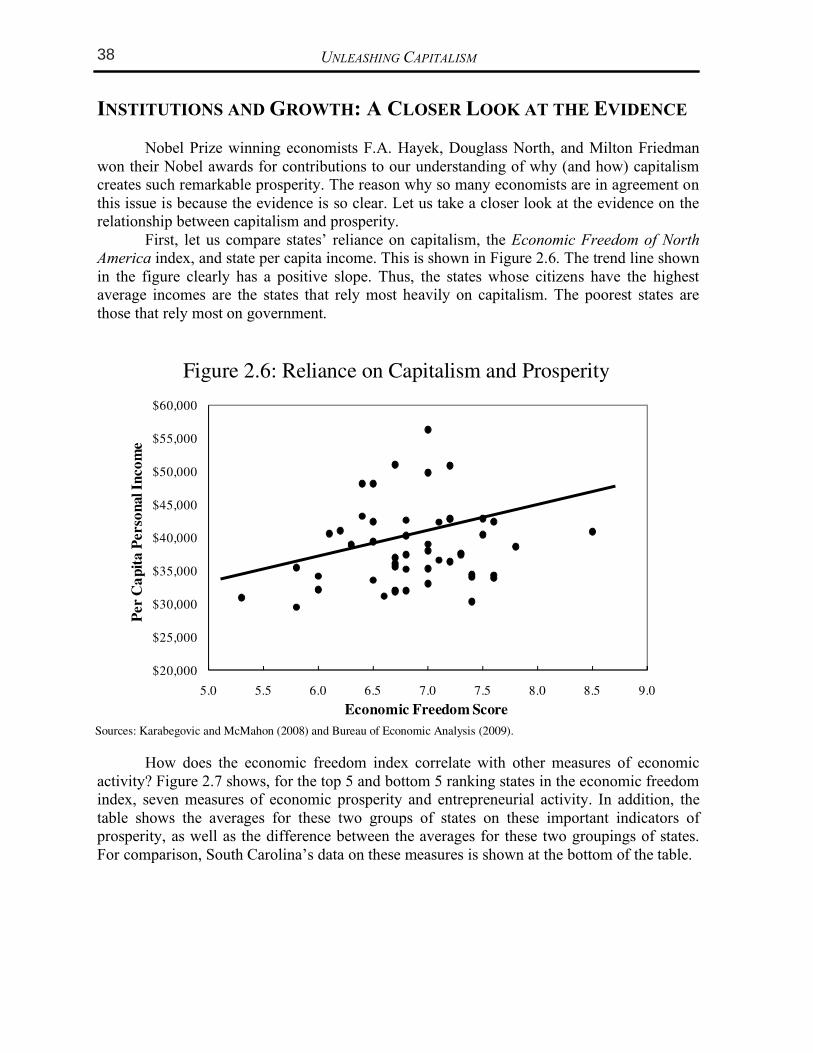
UNLEASHING CAPITALISM
INSTITUTIONS AND GROWTH: A CLOSER LOOK AT THE EVIDENCE
Nobel Prize winning economists F.A. Hayek, Douglass North, and Milton Friedman won their Nobel awards for contributions to our understanding of why (and how) capitalism creates such remarkable prosperity. The reason why so many economists are in agreement on this issue is because the evidence is so clear. Let us take a closer look at the evidence on the relationship between capitalism and prosperity. First, let us compare states’ reliance on capitalism, the Economic Freedom of North America index, and state per capita income. This is shown in Figure 2.6. The trend line shown in the figure clearly has a positive slope. Thus, the states whose citizens have the highest average incomes are the states that rely most heavily on capitalism. The poorest states are those that rely most on government.
Figure 2.6: Reliance on Capitalism and Prosperity
$20,000
$25,000
$30,000
$35,000
$40,000
$45,000
$50,000
$55,000
$60,000
5.0 5.5 6.0 6.5 7.0 7.5 8.0 8.5 9.0
Economic Freedom Score
Sources: Karabegovic and McMahon (2008) and Bureau of Economic Analysis (2009).
How does the economic freedom index correlate with other measures of economic activity? Figure 2.7 shows, for the top 5 and bottom 5 ranking states in the economic freedom index, seven measures of economic prosperity and entrepreneurial activity. In addition, the table shows the averages for these two groups of states on these important indicators of prosperity, as well as the difference between the averages for these two groupings of states. For comparison, South Carolina’s data on these measures is shown at the bottom of the table.
CHAPTER 2: THE SOURCES OF ECONOMIC GROWTH
Figure 2.7: Capitalism’s Economic Record
Measures of Entrepreneurial Activity (annual averages)
State Score
Rank
(among
U.S. states)
Per Capita
Personal
Income
(2008)
Poverty
Rate
(2007)
Venture
Capital
Investment
Per Capita
Patents Per
Capita (per
100,000
pop.)
Sole
Proprietorship
Growth Rate
Establishment
Birth Rate (all
firms)
Establishment
Birth Rate
(large firms
only)
Top 5 States
Delaware 8.5 1 $40,852 10.3% $60.97 52.6 5.5% 13.1% 14.2%
Texas 7.8 2 $38,575 16.3% $113.29 25.9 3.3% 12.8% 12.0%
Colorado 7.6 3 (tie) $42,377 11.5% $333.22 37.1 4.6% 14.2% 13.0%
Georgia 7.6 3 (tie) $33,975 14.3% $103.63 14.6 4.0% 13.5% 11.7%
North Carolina 7.6 3 (tie) $34,439 14.3% $82.57 19.5 3.5% 11.7% 10.3%
Bottom 5 States
Montana 6.0 46 (tie) $34,256 14.1% $14.30 12.6 1.9% 12.0% 10.7%
New Mexico 6.0 46 (tie) $32,091 17.9% $10.08 16.3 2.7% 12.1% 10.8%
Maine 5.8 48 (tie) $35,381 12.2% $34.96 9.3 3.0% 11.2% 9.5%
Mississippi 5.8 48 (tie) $29,569 20.7% $18.53 5.6 3.4% 11.1% 9.7%
West Virginia 5.3 50 $30,831 17.1% $0.00 0.0 2.8% 9.5% 8.6%
Average - Top 5 States $38,044 13.3% $138.74 29.9 4.2% 13.1% 12.2%
Average - Bottom 5 States $32,426 16.4% $15.57 8.8 2.8% 11.2% 9.9%
Difference (Top minus Bottom) $5,618 -3.1% $123.16 21.2 1.4% 1.9% 2.4%
For Comparison
South Carolina 6.8 25 $31,884 15.1% $22.98 13.2 2.4% 11.8% 9.7%
Economic
Performance
Measures
Economic Freedom
Index (2005)
Sources: Bureau of Economic Analysis (2009), Karabegovic and McMahon (2008), U.S. Census Bureau (2009), and Sobel (2008).
The states listed in the top of the table, those with the best institutions, are uniformly more prosperous than the states with the worst economic institutions. The differences in economic outcomes are striking. Looking at the averages given in the bottom of the table, average per capita personal income is $5,618 higher, and the poverty rate is 3.1 percentage points lower, on average, in those states with the best economic institutions. Examining the measures of entrepreneurial activity, a similar pattern emerges—states with the most economic freedom have higher rates of entrepreneurial activity. Relative to the states with the least economic freedom, those with the most have venture capital investment $123.16 higher per capita, a rate of patents 21.2 higher per 100,000 residents, a growth rate of sole proprietorships 1.4 percentage points higher, an establishment birth rate almost 2 percent higher, and a birth rate of large establishments 2.4 percentage points higher.
Because South Carolina ranks in the middle of the pack on economic freedom, the measures of entrepreneurship and prosperity for South Carolina generally fall in between the values for the top and bottom states. Of most interest, however, is probably how South Carolina compares to its neighboring states of Georgia and North Carolina (both listed among the top 5 states in Figure 2.7). As was mentioned earlier in this chapter, South Carolina lags behind its neighboring states on measures of entrepreneurial activity and prosperity.
UNLEASHING CAPITALISM
INSTITUTIONS AND GROWTH: A CLOSER LOOK AT THE EVIDENCE
Nobel Prize winning economists F.A. Hayek, Douglass North, and Milton Friedman won their Nobel awards for contributions to our understanding of why (and how) capitalism creates such remarkable prosperity. The reason why so many economists are in agreement on this issue is because the evidence is so clear. Let us take a closer look at the evidence on the relationship between capitalism and prosperity. First, let us compare states’ reliance on capitalism, the Economic Freedom of North America index, and state per capita income. This is shown in Figure 2.6. The trend line shown in the figure clearly has a positive slope. Thus, the states whose citizens have the highest average incomes are the states that rely most heavily on capitalism. The poorest states are those that rely most on government.
Figure 2.6: Reliance on Capitalism and Prosperity
$20,000
$25,000
$30,000
$35,000
$40,000
$45,000
$50,000
$55,000
$60,000
5.0 5.5 6.0 6.5 7.0 7.5 8.0 8.5 9.0
Per
Ca
pit
a P
erso
nal
In
com
e
Economic Freedom Score
Sources: Karabegovic and McMahon (2008) and Bureau of Economic Analysis (2009).
How does the economic freedom index correlate with other measures of economic activity? Figure 2.7 shows, for the top 5 and bottom 5 ranking states in the economic freedom index, seven measures of economic prosperity and entrepreneurial activity. In addition, the table shows the averages for these two groups of states on these important indicators of prosperity, as well as the difference between the averages for these two groupings of states. For comparison, South Carolina’s data on these measures is shown at the bottom of the table.
UNLEASHING CAPITALISM 18
manufacturing property tax in the country. In Figure 5.8 we present the effective property tax rates data for Southeastern states, for comparison. The ranks given for the states are out of all 50 states. The ‘net tax’ and ‘effective tax rate’ are calculated based on property valued at $25 million ($12.5 million in machinery and equipment, $12.5 million in inventories, and $2.5 million in fixtures). Notice that South Carolina’s effective tax rate on industrial property is over 7.8 times higher than the most industry-friendly state, Delaware. (Delaware is listed in the figure because it is the lowest-tax state.)
Figure 5.8: Industrial Property Taxes in Southeastern states*, 2007 State Rank (of 50) Net Tax Effective Tax Rate
South Carolina 1 $1,864,900 3.73%
Mississippi 4 $1,291,050 2.58%
Texas 6 $1,264,358 2.53%
Tennessee 10 $1,033,544 2.07%
West Virginia 14 $833,234 1.67%
Louisiana 17 $783,407 1.57%
Georgia 20 $760,381 1.52%
Florida 24 $677,683 1.36%
Alabama 35 $533,776 1.11%
North Carolina 37 $491,071 0.98%
Kentucky 47 $327,100 0.65%
Virginia 49 $241,498 0.48%
Delaware 50 $238,840 0.48%
Source: National Association of Manufacturers (2009) * Taxes measured in the states’ largest city only.
Importantly, South Carolina’s effective tax rate is almost 2.5 times greater than Georgia’s tax, and almost 4 times greater than North Carolina’s. This puts South Carolina at a serious disadvantage, in terms of its ability to attract and keep industry. Since South Carolina has the highest tax in the country on industrial property, it should be no surprise that it has one of the lowest per capita incomes and economic growth rates in the country. Although it is probably not critical that South Carolina set its tax rate to the lowest in the country, it should definitely make it at least competitive for the Southeast. Since Georgia’s rate is effectively 1.52 percent and North Carolina’s is just under 1 percent, a rate at around 1 percent might be sufficient to attract more industry. Working to reduce the various taxes applied to industry would seriously improve the state’s competitiveness. Such a significant reduction in taxes on industrial property would obviously lead to a reduction in tax revenues on industrial property, at least initially. However, the overall revenue may in fact increase once the growth rate in the state begins to pick up and more industry moves into the state. Furthermore, if the official tax rates are lowered, then the state
38 CHAPTER 5: SPECIFIC TAX REFORMS
13
Presumably the original intent of imposing a tax rate schedule with graduated marginal tax rates was to make the income tax progressive. However, what progressivity exists in the state’s income tax structure is due to the zero tax on the first $2,630 of income, and because of the graduated marginal tax rates. However, since the marginal tax rate increases over such small steps in income, as shown in Figure 5.5, most of the progressivity occurs at lower income levels, not higher levels of income. At higher income levels, the average tax rate hardly increases at all. This nature of the current tax is directly contradictory to the goal of progressivity. So although on the surface it appears that the tax satisfies the vertical equity condition, it really does this only at the lower income levels reducing the wealth of these lowest income taxpayers, not the intended consequence.
Figure 5.5: South Carolina income tax: Current tax rates compared to inflation-indexed rates, 2009
Current Income Tax
Rates/Brackets
Income Tax Rates/Brackets if 1959 Tax Schedule was Inflation Adjusted to
2009
Taxable Income Tax
Amount Average Tax Rate
Tax Amount
Average Tax Rate
$5,000 $71 1.42% $125 2.5%
$10,000 $290 2.90% $250 2.5%
$15,000 $604 4.03% $377 2.51%
$20,000 $954 4.77% $527 2.63%
$30,000 $1,654 5.51% $834 2.78%
$50,000 $3,054 6.10% $1,695 3.39%
$75,000 $4,804 6.41% $3,127 4.17%
$100,000 $6,554 6.56% $4,877 4.88%
$150,000 $10,054 6.70% $8,377 5.58%
$200,000 $13,554 6.77% $11,877 5.94%
Figure 5.5 also shows what the average tax rates are for various incomes and taxes
under the current tax system in South Carolina. In the right columns it also shows what the taxes and average tax rates would be if the 1959 tax tables were indexed for inflation. The figure clearly shows that the 1959 indexed tax rate structure is more uniformly progressive, especially at higher levels of incomes. It keeps tax rates extremely low for the lowest income individuals in the state. Figure 5.5 also shows that the current tax system charges all income groups more in taxes than an indexed rate schedule. The only exception is the $5,000 income earner in the table. As South Carolina income taxes continue to climb while the tax brackets remain stagnant, the state becomes a relatively high-tax state. This has a negative impact on
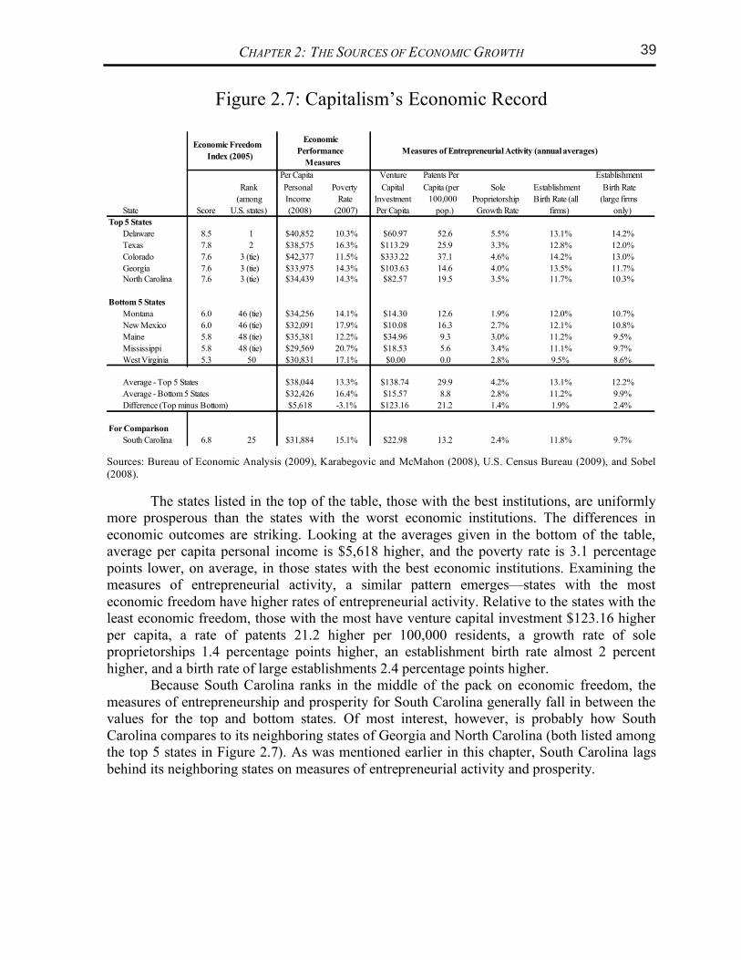
UNLEASHING CAPITALISM
INSTITUTIONS AND GROWTH: A CLOSER LOOK AT THE EVIDENCE
Nobel Prize winning economists F.A. Hayek, Douglass North, and Milton Friedman won their Nobel awards for contributions to our understanding of why (and how) capitalism creates such remarkable prosperity. The reason why so many economists are in agreement on this issue is because the evidence is so clear. Let us take a closer look at the evidence on the relationship between capitalism and prosperity. First, let us compare states’ reliance on capitalism, the Economic Freedom of North America index, and state per capita income. This is shown in Figure 2.6. The trend line shown in the figure clearly has a positive slope. Thus, the states whose citizens have the highest average incomes are the states that rely most heavily on capitalism. The poorest states are those that rely most on government.
Figure 2.6: Reliance on Capitalism and Prosperity
$20,000
$25,000
$30,000
$35,000
$40,000
$45,000
$50,000
$55,000
$60,000
5.0 5.5 6.0 6.5 7.0 7.5 8.0 8.5 9.0
Economic Freedom Score
Sources: Karabegovic and McMahon (2008) and Bureau of Economic Analysis (2009).
How does the economic freedom index correlate with other measures of economic activity? Figure 2.7 shows, for the top 5 and bottom 5 ranking states in the economic freedom index, seven measures of economic prosperity and entrepreneurial activity. In addition, the table shows the averages for these two groups of states on these important indicators of prosperity, as well as the difference between the averages for these two groupings of states. For comparison, South Carolina’s data on these measures is shown at the bottom of the table.
CHAPTER 2: THE SOURCES OF ECONOMIC GROWTH
Figure 2.7: Capitalism’s Economic Record
Measures of Entrepreneurial Activity (annual averages)
State Score
Rank
(among
U.S. states)
Per Capita
Personal
Income
(2008)
Poverty
Rate
(2007)
Venture
Capital
Investment
Per Capita
Patents Per
Capita (per
100,000
pop.)
Sole
Proprietorship
Growth Rate
Establishment
Birth Rate (all
firms)
Establishment
Birth Rate
(large firms
only)
Top 5 States
Delaware 8.5 1 $40,852 10.3% $60.97 52.6 5.5% 13.1% 14.2%
Texas 7.8 2 $38,575 16.3% $113.29 25.9 3.3% 12.8% 12.0%
Colorado 7.6 3 (tie) $42,377 11.5% $333.22 37.1 4.6% 14.2% 13.0%
Georgia 7.6 3 (tie) $33,975 14.3% $103.63 14.6 4.0% 13.5% 11.7%
North Carolina 7.6 3 (tie) $34,439 14.3% $82.57 19.5 3.5% 11.7% 10.3%
Bottom 5 States
Montana 6.0 46 (tie) $34,256 14.1% $14.30 12.6 1.9% 12.0% 10.7%
New Mexico 6.0 46 (tie) $32,091 17.9% $10.08 16.3 2.7% 12.1% 10.8%
Maine 5.8 48 (tie) $35,381 12.2% $34.96 9.3 3.0% 11.2% 9.5%
Mississippi 5.8 48 (tie) $29,569 20.7% $18.53 5.6 3.4% 11.1% 9.7%
West Virginia 5.3 50 $30,831 17.1% $0.00 0.0 2.8% 9.5% 8.6%
Average - Top 5 States $38,044 13.3% $138.74 29.9 4.2% 13.1% 12.2%
Average - Bottom 5 States $32,426 16.4% $15.57 8.8 2.8% 11.2% 9.9%
Difference (Top minus Bottom) $5,618 -3.1% $123.16 21.2 1.4% 1.9% 2.4%
For Comparison
South Carolina 6.8 25 $31,884 15.1% $22.98 13.2 2.4% 11.8% 9.7%
Economic
Performance
Measures
Economic Freedom
Index (2005)
Sources: Bureau of Economic Analysis (2009), Karabegovic and McMahon (2008), U.S. Census Bureau (2009), and Sobel (2008).
The states listed in the top of the table, those with the best institutions, are uniformly more prosperous than the states with the worst economic institutions. The differences in economic outcomes are striking. Looking at the averages given in the bottom of the table, average per capita personal income is $5,618 higher, and the poverty rate is 3.1 percentage points lower, on average, in those states with the best economic institutions. Examining the measures of entrepreneurial activity, a similar pattern emerges—states with the most economic freedom have higher rates of entrepreneurial activity. Relative to the states with the least economic freedom, those with the most have venture capital investment $123.16 higher per capita, a rate of patents 21.2 higher per 100,000 residents, a growth rate of sole proprietorships 1.4 percentage points higher, an establishment birth rate almost 2 percent higher, and a birth rate of large establishments 2.4 percentage points higher.
Because South Carolina ranks in the middle of the pack on economic freedom, the measures of entrepreneurship and prosperity for South Carolina generally fall in between the values for the top and bottom states. Of most interest, however, is probably how South Carolina compares to its neighboring states of Georgia and North Carolina (both listed among the top 5 states in Figure 2.7). As was mentioned earlier in this chapter, South Carolina lags behind its neighboring states on measures of entrepreneurial activity and prosperity.
UNLEASHING CAPITALISM 18
manufacturing property tax in the country. In Figure 5.8 we present the effective property tax rates data for Southeastern states, for comparison. The ranks given for the states are out of all 50 states. The ‘net tax’ and ‘effective tax rate’ are calculated based on property valued at $25 million ($12.5 million in machinery and equipment, $12.5 million in inventories, and $2.5 million in fixtures). Notice that South Carolina’s effective tax rate on industrial property is over 7.8 times higher than the most industry-friendly state, Delaware. (Delaware is listed in the figure because it is the lowest-tax state.)
Figure 5.8: Industrial Property Taxes in Southeastern states*, 2007 State Rank (of 50) Net Tax Effective Tax Rate
South Carolina 1 $1,864,900 3.73%
Mississippi 4 $1,291,050 2.58%
Texas 6 $1,264,358 2.53%
Tennessee 10 $1,033,544 2.07%
West Virginia 14 $833,234 1.67%
Louisiana 17 $783,407 1.57%
Georgia 20 $760,381 1.52%
Florida 24 $677,683 1.36%
Alabama 35 $533,776 1.11%
North Carolina 37 $491,071 0.98%
Kentucky 47 $327,100 0.65%
Virginia 49 $241,498 0.48%
Delaware 50 $238,840 0.48%
Source: National Association of Manufacturers (2009) * Taxes measured in the states’ largest city only.
Importantly, South Carolina’s effective tax rate is almost 2.5 times greater than Georgia’s tax, and almost 4 times greater than North Carolina’s. This puts South Carolina at a serious disadvantage, in terms of its ability to attract and keep industry. Since South Carolina has the highest tax in the country on industrial property, it should be no surprise that it has one of the lowest per capita incomes and economic growth rates in the country. Although it is probably not critical that South Carolina set its tax rate to the lowest in the country, it should definitely make it at least competitive for the Southeast. Since Georgia’s rate is effectively 1.52 percent and North Carolina’s is just under 1 percent, a rate at around 1 percent might be sufficient to attract more industry. Working to reduce the various taxes applied to industry would seriously improve the state’s competitiveness. Such a significant reduction in taxes on industrial property would obviously lead to a reduction in tax revenues on industrial property, at least initially. However, the overall revenue may in fact increase once the growth rate in the state begins to pick up and more industry moves into the state. Furthermore, if the official tax rates are lowered, then the state
39CHAPTER 5: SPECIFIC TAX REFORMS
13
Presumably the original intent of imposing a tax rate schedule with graduated marginal tax rates was to make the income tax progressive. However, what progressivity exists in the state’s income tax structure is due to the zero tax on the first $2,630 of income, and because of the graduated marginal tax rates. However, since the marginal tax rate increases over such small steps in income, as shown in Figure 5.5, most of the progressivity occurs at lower income levels, not higher levels of income. At higher income levels, the average tax rate hardly increases at all. This nature of the current tax is directly contradictory to the goal of progressivity. So although on the surface it appears that the tax satisfies the vertical equity condition, it really does this only at the lower income levels reducing the wealth of these lowest income taxpayers, not the intended consequence.
Figure 5.5: South Carolina income tax: Current tax rates compared to inflation-indexed rates, 2009
Current Income Tax
Rates/Brackets
Income Tax Rates/Brackets if 1959 Tax Schedule was Inflation Adjusted to
2009
Taxable Income Tax
Amount Average Tax Rate
Tax Amount
Average Tax Rate
$5,000 $71 1.42% $125 2.5%
$10,000 $290 2.90% $250 2.5%
$15,000 $604 4.03% $377 2.51%
$20,000 $954 4.77% $527 2.63%
$30,000 $1,654 5.51% $834 2.78%
$50,000 $3,054 6.10% $1,695 3.39%
$75,000 $4,804 6.41% $3,127 4.17%
$100,000 $6,554 6.56% $4,877 4.88%
$150,000 $10,054 6.70% $8,377 5.58%
$200,000 $13,554 6.77% $11,877 5.94%
Figure 5.5 also shows what the average tax rates are for various incomes and taxes
under the current tax system in South Carolina. In the right columns it also shows what the taxes and average tax rates would be if the 1959 tax tables were indexed for inflation. The figure clearly shows that the 1959 indexed tax rate structure is more uniformly progressive, especially at higher levels of incomes. It keeps tax rates extremely low for the lowest income individuals in the state. Figure 5.5 also shows that the current tax system charges all income groups more in taxes than an indexed rate schedule. The only exception is the $5,000 income earner in the table. As South Carolina income taxes continue to climb while the tax brackets remain stagnant, the state becomes a relatively high-tax state. This has a negative impact on
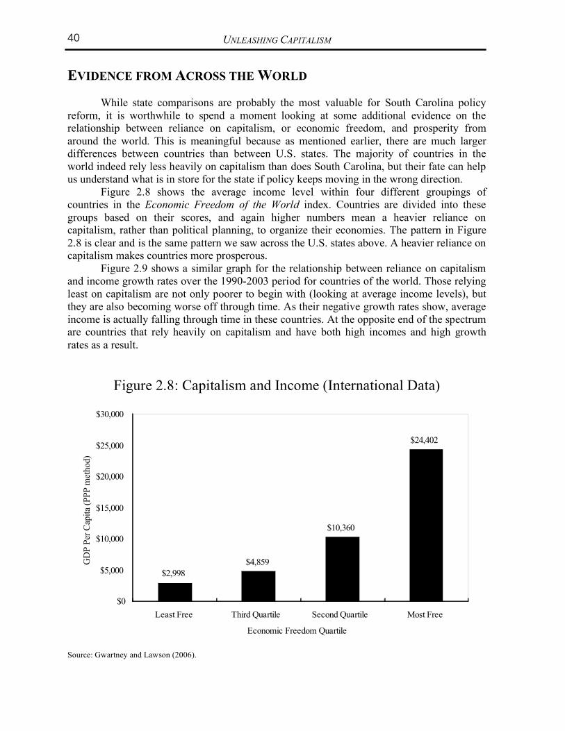
UNLEASHING CAPITALISM
EVIDENCE FROM ACROSS THE WORLD
While state comparisons are probably the most valuable for South Carolina policy reform, it is worthwhile to spend a moment looking at some additional evidence on the relationship between reliance on capitalism, or economic freedom, and prosperity from around the world. This is meaningful because as mentioned earlier, there are much larger differences between countries than between U.S. states. The majority of countries in the world indeed rely less heavily on capitalism than does South Carolina, but their fate can help us understand what is in store for the state if policy keeps moving in the wrong direction. Figure 2.8 shows the average income level within four different groupings of countries in the Economic Freedom of the World index. Countries are divided into these groups based on their scores, and again higher numbers mean a heavier reliance on capitalism, rather than political planning, to organize their economies. The pattern in Figure 2.8 is clear and is the same pattern we saw across the U.S. states above. A heavier reliance on capitalism makes countries more prosperous.
Figure 2.9 shows a similar graph for the relationship between reliance on capitalism and income growth rates over the 1990-2003 period for countries of the world. Those relying least on capitalism are not only poorer to begin with (looking at average income levels), but they are also becoming worse off through time. As their negative growth rates show, average income is actually falling through time in these countries. At the opposite end of the spectrum are countries that rely heavily on capitalism and have both high incomes and high growth rates as a result.
Figure 2.8: Capitalism and Income (International Data)
$2,998
$4,859
$10,360
$24,402
$0
$5,000
$10,000
$15,000
$20,000
$25,000
$30,000
Least Free Third Quartile Second Quartile Most Free
Economic Freedom Quartile
GD
P P
er C
apit
a (P
PP
met
hod)
Source: Gwartney and Lawson (2006).
CHAPTER 2: THE SOURCES OF ECONOMIC GROWTH
Figure 2.9: Capitalism and Growth (International Data)
-0.20%
1.50% 1.50%
2.10%
-0.50%
0.00%
0.50%
1.00%
1.50%
2.00%
2.50%
Least Free Third Quartile Second Quartile Most Free
Economic Freedom Quartile
Gro
wth
Rat
e of
Rea
l G
DP
Per
Cap
ita
(1990-2
003)
Source: Gwartney and Lawson (2006).
In summary, the international evidence bears out the same conclusions as the evidence
from U.S. states. Those areas embracing capitalism are richer and grow faster, and those areas that do not are poorer and grow slower.
THE GAP BETWEEN RICH AND POOR
This chapter has presented evidence that areas relying on capitalism—the protection of private property through limited political and sound legal institutions—are more prosperous. The data we have presented here on average per capita income supports this conclusion. Some readers, however, might worry that while reliance on capitalism causes average income to rise, it may cause the distribution of income among people to change in an undesirable direction. After all, opponents of capitalism in the popular media quote statistics about how the rich are getting richer and the poor are getting poorer. Would a heavier reliance on capitalism make this happen in South Carolina? First, it is important to differentiate between income disparities within a state changing and income disparities across states changing. For example, states (and countries) relying more heavily on capitalism have both higher levels of income and faster income growth, while states (and countries) relying less heavily on capitalism have both lower levels of income and slower economic growth. So it is true that through time, the relatively richer citizens of places like Delaware keep getting richer faster than the relatively poorer citizens of places like South Carolina. As Chapter 1 demonstrated, through time, even small differences
UNLEASHING CAPITALISM 18
manufacturing property tax in the country. In Figure 5.8 we present the effective property tax rates data for Southeastern states, for comparison. The ranks given for the states are out of all 50 states. The ‘net tax’ and ‘effective tax rate’ are calculated based on property valued at $25 million ($12.5 million in machinery and equipment, $12.5 million in inventories, and $2.5 million in fixtures). Notice that South Carolina’s effective tax rate on industrial property is over 7.8 times higher than the most industry-friendly state, Delaware. (Delaware is listed in the figure because it is the lowest-tax state.)
Figure 5.8: Industrial Property Taxes in Southeastern states*, 2007 State Rank (of 50) Net Tax Effective Tax Rate
South Carolina 1 $1,864,900 3.73%
Mississippi 4 $1,291,050 2.58%
Texas 6 $1,264,358 2.53%
Tennessee 10 $1,033,544 2.07%
West Virginia 14 $833,234 1.67%
Louisiana 17 $783,407 1.57%
Georgia 20 $760,381 1.52%
Florida 24 $677,683 1.36%
Alabama 35 $533,776 1.11%
North Carolina 37 $491,071 0.98%
Kentucky 47 $327,100 0.65%
Virginia 49 $241,498 0.48%
Delaware 50 $238,840 0.48%
Source: National Association of Manufacturers (2009) * Taxes measured in the states’ largest city only.
Importantly, South Carolina’s effective tax rate is almost 2.5 times greater than Georgia’s tax, and almost 4 times greater than North Carolina’s. This puts South Carolina at a serious disadvantage, in terms of its ability to attract and keep industry. Since South Carolina has the highest tax in the country on industrial property, it should be no surprise that it has one of the lowest per capita incomes and economic growth rates in the country. Although it is probably not critical that South Carolina set its tax rate to the lowest in the country, it should definitely make it at least competitive for the Southeast. Since Georgia’s rate is effectively 1.52 percent and North Carolina’s is just under 1 percent, a rate at around 1 percent might be sufficient to attract more industry. Working to reduce the various taxes applied to industry would seriously improve the state’s competitiveness. Such a significant reduction in taxes on industrial property would obviously lead to a reduction in tax revenues on industrial property, at least initially. However, the overall revenue may in fact increase once the growth rate in the state begins to pick up and more industry moves into the state. Furthermore, if the official tax rates are lowered, then the state
40 CHAPTER 5: SPECIFIC TAX REFORMS
13
Presumably the original intent of imposing a tax rate schedule with graduated marginal tax rates was to make the income tax progressive. However, what progressivity exists in the state’s income tax structure is due to the zero tax on the first $2,630 of income, and because of the graduated marginal tax rates. However, since the marginal tax rate increases over such small steps in income, as shown in Figure 5.5, most of the progressivity occurs at lower income levels, not higher levels of income. At higher income levels, the average tax rate hardly increases at all. This nature of the current tax is directly contradictory to the goal of progressivity. So although on the surface it appears that the tax satisfies the vertical equity condition, it really does this only at the lower income levels reducing the wealth of these lowest income taxpayers, not the intended consequence.
Figure 5.5: South Carolina income tax: Current tax rates compared to inflation-indexed rates, 2009
Current Income Tax
Rates/Brackets
Income Tax Rates/Brackets if 1959 Tax Schedule was Inflation Adjusted to
2009
Taxable Income Tax
Amount Average Tax Rate
Tax Amount
Average Tax Rate
$5,000 $71 1.42% $125 2.5%
$10,000 $290 2.90% $250 2.5%
$15,000 $604 4.03% $377 2.51%
$20,000 $954 4.77% $527 2.63%
$30,000 $1,654 5.51% $834 2.78%
$50,000 $3,054 6.10% $1,695 3.39%
$75,000 $4,804 6.41% $3,127 4.17%
$100,000 $6,554 6.56% $4,877 4.88%
$150,000 $10,054 6.70% $8,377 5.58%
$200,000 $13,554 6.77% $11,877 5.94%
Figure 5.5 also shows what the average tax rates are for various incomes and taxes
under the current tax system in South Carolina. In the right columns it also shows what the taxes and average tax rates would be if the 1959 tax tables were indexed for inflation. The figure clearly shows that the 1959 indexed tax rate structure is more uniformly progressive, especially at higher levels of incomes. It keeps tax rates extremely low for the lowest income individuals in the state. Figure 5.5 also shows that the current tax system charges all income groups more in taxes than an indexed rate schedule. The only exception is the $5,000 income earner in the table. As South Carolina income taxes continue to climb while the tax brackets remain stagnant, the state becomes a relatively high-tax state. This has a negative impact on
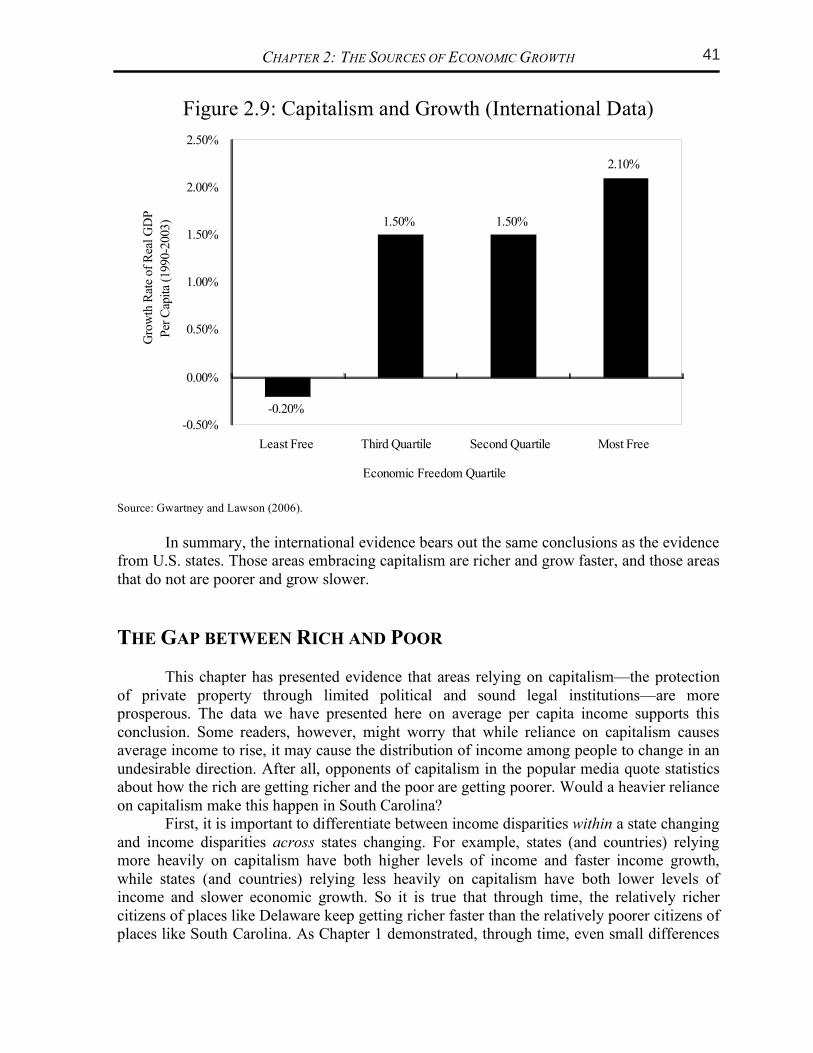
UNLEASHING CAPITALISM
EVIDENCE FROM ACROSS THE WORLD
While state comparisons are probably the most valuable for South Carolina policy reform, it is worthwhile to spend a moment looking at some additional evidence on the relationship between reliance on capitalism, or economic freedom, and prosperity from around the world. This is meaningful because as mentioned earlier, there are much larger differences between countries than between U.S. states. The majority of countries in the world indeed rely less heavily on capitalism than does South Carolina, but their fate can help us understand what is in store for the state if policy keeps moving in the wrong direction. Figure 2.8 shows the average income level within four different groupings of countries in the Economic Freedom of the World index. Countries are divided into these groups based on their scores, and again higher numbers mean a heavier reliance on capitalism, rather than political planning, to organize their economies. The pattern in Figure 2.8 is clear and is the same pattern we saw across the U.S. states above. A heavier reliance on capitalism makes countries more prosperous.
Figure 2.9 shows a similar graph for the relationship between reliance on capitalism and income growth rates over the 1990-2003 period for countries of the world. Those relying least on capitalism are not only poorer to begin with (looking at average income levels), but they are also becoming worse off through time. As their negative growth rates show, average income is actually falling through time in these countries. At the opposite end of the spectrum are countries that rely heavily on capitalism and have both high incomes and high growth rates as a result.
Figure 2.8: Capitalism and Income (International Data)
$2,998
$4,859
$10,360
$24,402
$0
$5,000
$10,000
$15,000
$20,000
$25,000
$30,000
Least Free Third Quartile Second Quartile Most Free
Economic Freedom Quartile
GD
P P
er C
apit
a (P
PP
met
hod)
Source: Gwartney and Lawson (2006).
CHAPTER 2: THE SOURCES OF ECONOMIC GROWTH
Figure 2.9: Capitalism and Growth (International Data)
-0.20%
1.50% 1.50%
2.10%
-0.50%
0.00%
0.50%
1.00%
1.50%
2.00%
2.50%
Least Free Third Quartile Second Quartile Most Free
Economic Freedom Quartile
Gro
wth
Rat
e of
Rea
l G
DP
Per
Cap
ita
(1990-2
003)
Source: Gwartney and Lawson (2006).
In summary, the international evidence bears out the same conclusions as the evidence
from U.S. states. Those areas embracing capitalism are richer and grow faster, and those areas that do not are poorer and grow slower.
THE GAP BETWEEN RICH AND POOR
This chapter has presented evidence that areas relying on capitalism—the protection of private property through limited political and sound legal institutions—are more prosperous. The data we have presented here on average per capita income supports this conclusion. Some readers, however, might worry that while reliance on capitalism causes average income to rise, it may cause the distribution of income among people to change in an undesirable direction. After all, opponents of capitalism in the popular media quote statistics about how the rich are getting richer and the poor are getting poorer. Would a heavier reliance on capitalism make this happen in South Carolina? First, it is important to differentiate between income disparities within a state changing and income disparities across states changing. For example, states (and countries) relying more heavily on capitalism have both higher levels of income and faster income growth, while states (and countries) relying less heavily on capitalism have both lower levels of income and slower economic growth. So it is true that through time, the relatively richer citizens of places like Delaware keep getting richer faster than the relatively poorer citizens of places like South Carolina. As Chapter 1 demonstrated, through time, even small differences
UNLEASHING CAPITALISM 18
manufacturing property tax in the country. In Figure 5.8 we present the effective property tax rates data for Southeastern states, for comparison. The ranks given for the states are out of all 50 states. The ‘net tax’ and ‘effective tax rate’ are calculated based on property valued at $25 million ($12.5 million in machinery and equipment, $12.5 million in inventories, and $2.5 million in fixtures). Notice that South Carolina’s effective tax rate on industrial property is over 7.8 times higher than the most industry-friendly state, Delaware. (Delaware is listed in the figure because it is the lowest-tax state.)
Figure 5.8: Industrial Property Taxes in Southeastern states*, 2007 State Rank (of 50) Net Tax Effective Tax Rate
South Carolina 1 $1,864,900 3.73%
Mississippi 4 $1,291,050 2.58%
Texas 6 $1,264,358 2.53%
Tennessee 10 $1,033,544 2.07%
West Virginia 14 $833,234 1.67%
Louisiana 17 $783,407 1.57%
Georgia 20 $760,381 1.52%
Florida 24 $677,683 1.36%
Alabama 35 $533,776 1.11%
North Carolina 37 $491,071 0.98%
Kentucky 47 $327,100 0.65%
Virginia 49 $241,498 0.48%
Delaware 50 $238,840 0.48%
Source: National Association of Manufacturers (2009) * Taxes measured in the states’ largest city only.
Importantly, South Carolina’s effective tax rate is almost 2.5 times greater than Georgia’s tax, and almost 4 times greater than North Carolina’s. This puts South Carolina at a serious disadvantage, in terms of its ability to attract and keep industry. Since South Carolina has the highest tax in the country on industrial property, it should be no surprise that it has one of the lowest per capita incomes and economic growth rates in the country. Although it is probably not critical that South Carolina set its tax rate to the lowest in the country, it should definitely make it at least competitive for the Southeast. Since Georgia’s rate is effectively 1.52 percent and North Carolina’s is just under 1 percent, a rate at around 1 percent might be sufficient to attract more industry. Working to reduce the various taxes applied to industry would seriously improve the state’s competitiveness. Such a significant reduction in taxes on industrial property would obviously lead to a reduction in tax revenues on industrial property, at least initially. However, the overall revenue may in fact increase once the growth rate in the state begins to pick up and more industry moves into the state. Furthermore, if the official tax rates are lowered, then the state
41CHAPTER 5: SPECIFIC TAX REFORMS
13
Presumably the original intent of imposing a tax rate schedule with graduated marginal tax rates was to make the income tax progressive. However, what progressivity exists in the state’s income tax structure is due to the zero tax on the first $2,630 of income, and because of the graduated marginal tax rates. However, since the marginal tax rate increases over such small steps in income, as shown in Figure 5.5, most of the progressivity occurs at lower income levels, not higher levels of income. At higher income levels, the average tax rate hardly increases at all. This nature of the current tax is directly contradictory to the goal of progressivity. So although on the surface it appears that the tax satisfies the vertical equity condition, it really does this only at the lower income levels reducing the wealth of these lowest income taxpayers, not the intended consequence.
Figure 5.5: South Carolina income tax: Current tax rates compared to inflation-indexed rates, 2009
Current Income Tax
Rates/Brackets
Income Tax Rates/Brackets if 1959 Tax Schedule was Inflation Adjusted to
2009
Taxable Income Tax
Amount Average Tax Rate
Tax Amount
Average Tax Rate
$5,000 $71 1.42% $125 2.5%
$10,000 $290 2.90% $250 2.5%
$15,000 $604 4.03% $377 2.51%
$20,000 $954 4.77% $527 2.63%
$30,000 $1,654 5.51% $834 2.78%
$50,000 $3,054 6.10% $1,695 3.39%
$75,000 $4,804 6.41% $3,127 4.17%
$100,000 $6,554 6.56% $4,877 4.88%
$150,000 $10,054 6.70% $8,377 5.58%
$200,000 $13,554 6.77% $11,877 5.94%
Figure 5.5 also shows what the average tax rates are for various incomes and taxes
under the current tax system in South Carolina. In the right columns it also shows what the taxes and average tax rates would be if the 1959 tax tables were indexed for inflation. The figure clearly shows that the 1959 indexed tax rate structure is more uniformly progressive, especially at higher levels of incomes. It keeps tax rates extremely low for the lowest income individuals in the state. Figure 5.5 also shows that the current tax system charges all income groups more in taxes than an indexed rate schedule. The only exception is the $5,000 income earner in the table. As South Carolina income taxes continue to climb while the tax brackets remain stagnant, the state becomes a relatively high-tax state. This has a negative impact on
UNLEASHING CAPITALISM
in growth rates can cause large differences in prosperity. However, this is the result of some areas getting policy to work properly. States that adopt good policies not only make their citizens richer, but those citizens keep getting even wealthier through time. States adopting bad policies make their citizens poorer and also cause them to experience slower growth, leaving them behind the progress of others. In other words, it is differences in the reliance on capitalism that explain the growing disparities across states. While the growing disparities across states are caused by policy differences in whether states embrace capitalism, the impact of a greater reliance on capitalism within a given state is a different story altogether. While certainly under capitalism some earn more than others, the alternative to this, the political allocation of wealth, is actually much more uneven. The benefits of government spending and transfers are much more highly concentrated among the politically powerful than are the benefits of private economic activity. The larger the government control of the economy, the more concentrated and uneven is income growth.
Let us look at the evidence.13 Consider the comparison of West Virginia—the state ranking 50th in the index of economic freedom—versus Delaware—the state ranking 1st. It is worth noting that these two states also rank 50th and 1st respectively in one of the alternative measures of state reliance on capitalism presented earlier in this chapter—the Institute for Legal Reform’s State Liability Systems Ranking of state legal systems. While the economic freedom index is certainly the closest measure to what economists mean by capitalism, because the most fundamental underpinning for capitalism is secure property rights (which are to a great degree determined by precedent through the state’s court decisions) the Institute for Legal Reform’s ranking of state legal systems provides another measure.
There is no question that both studies are in agreement as to these two states comprising the two extremes: Delaware is the best example of capitalism in the United States and West Virginia is the best example of the lack of free markets. From the government spending data presented earlier, in West Virginia government spending exceeds 50 percent of the economy, while in Delaware it is only 20 percent. Let us compare how income growth varies across the income distribution in Delaware and West Virginia.
Figure 2.10 shows data on how the growth of income has differed among income classes in West Virginia over the last two decades. Income growth has been very uneven in West Virginia. The poorest 20 percent of West Virginians experienced income growth of approximately 11 percent, in total, over the past two decades. Moving to the right, higher income groups saw income rise even faster. The richest 20 percent of West Virginians experienced a 63 percent increase in income over this period, a growth rate almost six times as large as for the lowest 20 percent.
Now, let us consider income growth in Delaware. As we have seen, Delaware’s government size, relative to its economy, is less than half as large as West Virginia, and it has one of the most favorable business climates in the United States, with very low labor and business regulations and a highly-rated legal system. As Figure 2.11 shows, income growth in Delaware has been much more even.
The income growth for the poorest 20 percent of Delaware’s population was almost 30 percent, a rate similar to all other income groups, including the richest 20 percent. Over the past two decades, those with the lowest incomes in Delaware have seen their incomes grow
13 Income growth data are from Bernstein, McNichol and Lyons (2006). Online at: http://www.epinet.org. For a
more scientific treatment of this issue, using data from all 50 states, see Ashby and Sobel (2006).
CHAPTER 2: THE SOURCES OF ECONOMIC GROWTH
by almost three times as much as those with the lowest incomes in West Virginia. Capitalism, as Delaware illustrates, is a rising tide that lifts all boats.
Figure 2.10: West Virginia Income Growth
10.7%12.9%
19.3%
30.0%
62.9%
0.00%
10.00%
20.00%
30.00%
40.00%
50.00%
60.00%
70.00%
Bottom 20% Fourth 20% Middle 20% Second 20% Top 20%
Income Quintile
Per
cen
t G
row
th i
n A
ver
ge
Inco
me
by
Qu
inti
le
(la
st t
wo
dec
ades
)
Figure 2.11: Delaware Income Growth
29.7%31.1%
28.4% 28.3%
39.3%
0.00%
5.00%
10.00%
15.00%
20.00%
25.00%
30.00%
35.00%
40.00%
45.00%
Bottom 20% Fourth 20% Middle 20% Second 20% Top 20%
Income Quintile
Per
cent
Gro
wth
in A
ver
ge
Inco
me
by
Qu
inti
le
(las
t tw
o d
ecad
es)
Sources for both figures: Taken from Sobel and Hall (2007) using data from Bernstein, McNichol and Lyons (2006) and Bureau of Economic Analysis (2006).
UNLEASHING CAPITALISM 18
manufacturing property tax in the country. In Figure 5.8 we present the effective property tax rates data for Southeastern states, for comparison. The ranks given for the states are out of all 50 states. The ‘net tax’ and ‘effective tax rate’ are calculated based on property valued at $25 million ($12.5 million in machinery and equipment, $12.5 million in inventories, and $2.5 million in fixtures). Notice that South Carolina’s effective tax rate on industrial property is over 7.8 times higher than the most industry-friendly state, Delaware. (Delaware is listed in the figure because it is the lowest-tax state.)
Figure 5.8: Industrial Property Taxes in Southeastern states*, 2007 State Rank (of 50) Net Tax Effective Tax Rate
South Carolina 1 $1,864,900 3.73%
Mississippi 4 $1,291,050 2.58%
Texas 6 $1,264,358 2.53%
Tennessee 10 $1,033,544 2.07%
West Virginia 14 $833,234 1.67%
Louisiana 17 $783,407 1.57%
Georgia 20 $760,381 1.52%
Florida 24 $677,683 1.36%
Alabama 35 $533,776 1.11%
North Carolina 37 $491,071 0.98%
Kentucky 47 $327,100 0.65%
Virginia 49 $241,498 0.48%
Delaware 50 $238,840 0.48%
Source: National Association of Manufacturers (2009) * Taxes measured in the states’ largest city only.
Importantly, South Carolina’s effective tax rate is almost 2.5 times greater than Georgia’s tax, and almost 4 times greater than North Carolina’s. This puts South Carolina at a serious disadvantage, in terms of its ability to attract and keep industry. Since South Carolina has the highest tax in the country on industrial property, it should be no surprise that it has one of the lowest per capita incomes and economic growth rates in the country. Although it is probably not critical that South Carolina set its tax rate to the lowest in the country, it should definitely make it at least competitive for the Southeast. Since Georgia’s rate is effectively 1.52 percent and North Carolina’s is just under 1 percent, a rate at around 1 percent might be sufficient to attract more industry. Working to reduce the various taxes applied to industry would seriously improve the state’s competitiveness. Such a significant reduction in taxes on industrial property would obviously lead to a reduction in tax revenues on industrial property, at least initially. However, the overall revenue may in fact increase once the growth rate in the state begins to pick up and more industry moves into the state. Furthermore, if the official tax rates are lowered, then the state
42 CHAPTER 5: SPECIFIC TAX REFORMS
13
Presumably the original intent of imposing a tax rate schedule with graduated marginal tax rates was to make the income tax progressive. However, what progressivity exists in the state’s income tax structure is due to the zero tax on the first $2,630 of income, and because of the graduated marginal tax rates. However, since the marginal tax rate increases over such small steps in income, as shown in Figure 5.5, most of the progressivity occurs at lower income levels, not higher levels of income. At higher income levels, the average tax rate hardly increases at all. This nature of the current tax is directly contradictory to the goal of progressivity. So although on the surface it appears that the tax satisfies the vertical equity condition, it really does this only at the lower income levels reducing the wealth of these lowest income taxpayers, not the intended consequence.
Figure 5.5: South Carolina income tax: Current tax rates compared to inflation-indexed rates, 2009
Current Income Tax
Rates/Brackets
Income Tax Rates/Brackets if 1959 Tax Schedule was Inflation Adjusted to
2009
Taxable Income Tax
Amount Average Tax Rate
Tax Amount
Average Tax Rate
$5,000 $71 1.42% $125 2.5%
$10,000 $290 2.90% $250 2.5%
$15,000 $604 4.03% $377 2.51%
$20,000 $954 4.77% $527 2.63%
$30,000 $1,654 5.51% $834 2.78%
$50,000 $3,054 6.10% $1,695 3.39%
$75,000 $4,804 6.41% $3,127 4.17%
$100,000 $6,554 6.56% $4,877 4.88%
$150,000 $10,054 6.70% $8,377 5.58%
$200,000 $13,554 6.77% $11,877 5.94%
Figure 5.5 also shows what the average tax rates are for various incomes and taxes
under the current tax system in South Carolina. In the right columns it also shows what the taxes and average tax rates would be if the 1959 tax tables were indexed for inflation. The figure clearly shows that the 1959 indexed tax rate structure is more uniformly progressive, especially at higher levels of incomes. It keeps tax rates extremely low for the lowest income individuals in the state. Figure 5.5 also shows that the current tax system charges all income groups more in taxes than an indexed rate schedule. The only exception is the $5,000 income earner in the table. As South Carolina income taxes continue to climb while the tax brackets remain stagnant, the state becomes a relatively high-tax state. This has a negative impact on
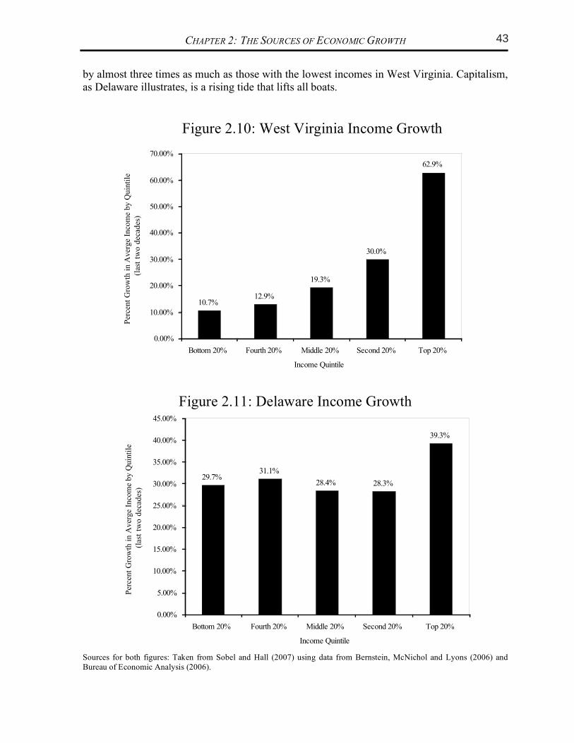
UNLEASHING CAPITALISM
in growth rates can cause large differences in prosperity. However, this is the result of some areas getting policy to work properly. States that adopt good policies not only make their citizens richer, but those citizens keep getting even wealthier through time. States adopting bad policies make their citizens poorer and also cause them to experience slower growth, leaving them behind the progress of others. In other words, it is differences in the reliance on capitalism that explain the growing disparities across states. While the growing disparities across states are caused by policy differences in whether states embrace capitalism, the impact of a greater reliance on capitalism within a given state is a different story altogether. While certainly under capitalism some earn more than others, the alternative to this, the political allocation of wealth, is actually much more uneven. The benefits of government spending and transfers are much more highly concentrated among the politically powerful than are the benefits of private economic activity. The larger the government control of the economy, the more concentrated and uneven is income growth.
Let us look at the evidence.13 Consider the comparison of West Virginia—the state ranking 50th in the index of economic freedom—versus Delaware—the state ranking 1st. It is worth noting that these two states also rank 50th and 1st respectively in one of the alternative measures of state reliance on capitalism presented earlier in this chapter—the Institute for Legal Reform’s State Liability Systems Ranking of state legal systems. While the economic freedom index is certainly the closest measure to what economists mean by capitalism, because the most fundamental underpinning for capitalism is secure property rights (which are to a great degree determined by precedent through the state’s court decisions) the Institute for Legal Reform’s ranking of state legal systems provides another measure.
There is no question that both studies are in agreement as to these two states comprising the two extremes: Delaware is the best example of capitalism in the United States and West Virginia is the best example of the lack of free markets. From the government spending data presented earlier, in West Virginia government spending exceeds 50 percent of the economy, while in Delaware it is only 20 percent. Let us compare how income growth varies across the income distribution in Delaware and West Virginia.
Figure 2.10 shows data on how the growth of income has differed among income classes in West Virginia over the last two decades. Income growth has been very uneven in West Virginia. The poorest 20 percent of West Virginians experienced income growth of approximately 11 percent, in total, over the past two decades. Moving to the right, higher income groups saw income rise even faster. The richest 20 percent of West Virginians experienced a 63 percent increase in income over this period, a growth rate almost six times as large as for the lowest 20 percent.
Now, let us consider income growth in Delaware. As we have seen, Delaware’s government size, relative to its economy, is less than half as large as West Virginia, and it has one of the most favorable business climates in the United States, with very low labor and business regulations and a highly-rated legal system. As Figure 2.11 shows, income growth in Delaware has been much more even.
The income growth for the poorest 20 percent of Delaware’s population was almost 30 percent, a rate similar to all other income groups, including the richest 20 percent. Over the past two decades, those with the lowest incomes in Delaware have seen their incomes grow
13 Income growth data are from Bernstein, McNichol and Lyons (2006). Online at: http://www.epinet.org. For a
more scientific treatment of this issue, using data from all 50 states, see Ashby and Sobel (2006).
CHAPTER 2: THE SOURCES OF ECONOMIC GROWTH
by almost three times as much as those with the lowest incomes in West Virginia. Capitalism, as Delaware illustrates, is a rising tide that lifts all boats.
Figure 2.10: West Virginia Income Growth
10.7%12.9%
19.3%
30.0%
62.9%
0.00%
10.00%
20.00%
30.00%
40.00%
50.00%
60.00%
70.00%
Bottom 20% Fourth 20% Middle 20% Second 20% Top 20%
Income Quintile
Per
cen
t G
row
th i
n A
ver
ge
Inco
me
by
Qu
inti
le
(la
st t
wo
dec
ades
)
Figure 2.11: Delaware Income Growth
29.7%31.1%
28.4% 28.3%
39.3%
0.00%
5.00%
10.00%
15.00%
20.00%
25.00%
30.00%
35.00%
40.00%
45.00%
Bottom 20% Fourth 20% Middle 20% Second 20% Top 20%
Income Quintile
Per
cent
Gro
wth
in A
ver
ge
Inco
me
by
Qu
inti
le
(las
t tw
o d
ecad
es)
Sources for both figures: Taken from Sobel and Hall (2007) using data from Bernstein, McNichol and Lyons (2006) and Bureau of Economic Analysis (2006).
UNLEASHING CAPITALISM 18
manufacturing property tax in the country. In Figure 5.8 we present the effective property tax rates data for Southeastern states, for comparison. The ranks given for the states are out of all 50 states. The ‘net tax’ and ‘effective tax rate’ are calculated based on property valued at $25 million ($12.5 million in machinery and equipment, $12.5 million in inventories, and $2.5 million in fixtures). Notice that South Carolina’s effective tax rate on industrial property is over 7.8 times higher than the most industry-friendly state, Delaware. (Delaware is listed in the figure because it is the lowest-tax state.)
Figure 5.8: Industrial Property Taxes in Southeastern states*, 2007 State Rank (of 50) Net Tax Effective Tax Rate
South Carolina 1 $1,864,900 3.73%
Mississippi 4 $1,291,050 2.58%
Texas 6 $1,264,358 2.53%
Tennessee 10 $1,033,544 2.07%
West Virginia 14 $833,234 1.67%
Louisiana 17 $783,407 1.57%
Georgia 20 $760,381 1.52%
Florida 24 $677,683 1.36%
Alabama 35 $533,776 1.11%
North Carolina 37 $491,071 0.98%
Kentucky 47 $327,100 0.65%
Virginia 49 $241,498 0.48%
Delaware 50 $238,840 0.48%
Source: National Association of Manufacturers (2009) * Taxes measured in the states’ largest city only.
Importantly, South Carolina’s effective tax rate is almost 2.5 times greater than Georgia’s tax, and almost 4 times greater than North Carolina’s. This puts South Carolina at a serious disadvantage, in terms of its ability to attract and keep industry. Since South Carolina has the highest tax in the country on industrial property, it should be no surprise that it has one of the lowest per capita incomes and economic growth rates in the country. Although it is probably not critical that South Carolina set its tax rate to the lowest in the country, it should definitely make it at least competitive for the Southeast. Since Georgia’s rate is effectively 1.52 percent and North Carolina’s is just under 1 percent, a rate at around 1 percent might be sufficient to attract more industry. Working to reduce the various taxes applied to industry would seriously improve the state’s competitiveness. Such a significant reduction in taxes on industrial property would obviously lead to a reduction in tax revenues on industrial property, at least initially. However, the overall revenue may in fact increase once the growth rate in the state begins to pick up and more industry moves into the state. Furthermore, if the official tax rates are lowered, then the state
43CHAPTER 5: SPECIFIC TAX REFORMS
13
Presumably the original intent of imposing a tax rate schedule with graduated marginal tax rates was to make the income tax progressive. However, what progressivity exists in the state’s income tax structure is due to the zero tax on the first $2,630 of income, and because of the graduated marginal tax rates. However, since the marginal tax rate increases over such small steps in income, as shown in Figure 5.5, most of the progressivity occurs at lower income levels, not higher levels of income. At higher income levels, the average tax rate hardly increases at all. This nature of the current tax is directly contradictory to the goal of progressivity. So although on the surface it appears that the tax satisfies the vertical equity condition, it really does this only at the lower income levels reducing the wealth of these lowest income taxpayers, not the intended consequence.
Figure 5.5: South Carolina income tax: Current tax rates compared to inflation-indexed rates, 2009
Current Income Tax
Rates/Brackets
Income Tax Rates/Brackets if 1959 Tax Schedule was Inflation Adjusted to
2009
Taxable Income Tax
Amount Average Tax Rate
Tax Amount
Average Tax Rate
$5,000 $71 1.42% $125 2.5%
$10,000 $290 2.90% $250 2.5%
$15,000 $604 4.03% $377 2.51%
$20,000 $954 4.77% $527 2.63%
$30,000 $1,654 5.51% $834 2.78%
$50,000 $3,054 6.10% $1,695 3.39%
$75,000 $4,804 6.41% $3,127 4.17%
$100,000 $6,554 6.56% $4,877 4.88%
$150,000 $10,054 6.70% $8,377 5.58%
$200,000 $13,554 6.77% $11,877 5.94%
Figure 5.5 also shows what the average tax rates are for various incomes and taxes
under the current tax system in South Carolina. In the right columns it also shows what the taxes and average tax rates would be if the 1959 tax tables were indexed for inflation. The figure clearly shows that the 1959 indexed tax rate structure is more uniformly progressive, especially at higher levels of incomes. It keeps tax rates extremely low for the lowest income individuals in the state. Figure 5.5 also shows that the current tax system charges all income groups more in taxes than an indexed rate schedule. The only exception is the $5,000 income earner in the table. As South Carolina income taxes continue to climb while the tax brackets remain stagnant, the state becomes a relatively high-tax state. This has a negative impact on
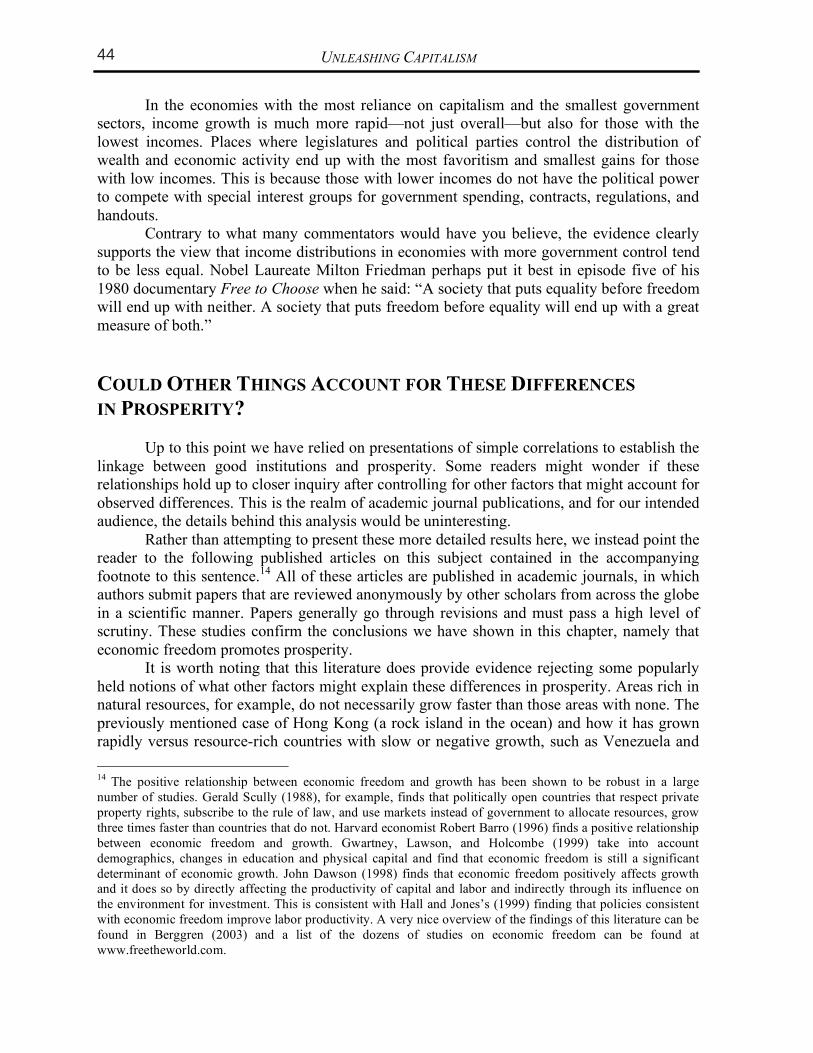
UNLEASHING CAPITALISM
In the economies with the most reliance on capitalism and the smallest government sectors, income growth is much more rapid—not just overall—but also for those with the lowest incomes. Places where legislatures and political parties control the distribution of wealth and economic activity end up with the most favoritism and smallest gains for those with low incomes. This is because those with lower incomes do not have the political power to compete with special interest groups for government spending, contracts, regulations, and handouts.
Contrary to what many commentators would have you believe, the evidence clearly supports the view that income distributions in economies with more government control tend to be less equal. Nobel Laureate Milton Friedman perhaps put it best in episode five of his 1980 documentary Free to Choose when he said: “A society that puts equality before freedom will end up with neither. A society that puts freedom before equality will end up with a great measure of both.”
COULD OTHER THINGS ACCOUNT FOR THESE DIFFERENCES
IN PROSPERITY?
Up to this point we have relied on presentations of simple correlations to establish the linkage between good institutions and prosperity. Some readers might wonder if these relationships hold up to closer inquiry after controlling for other factors that might account for observed differences. This is the realm of academic journal publications, and for our intended audience, the details behind this analysis would be uninteresting. Rather than attempting to present these more detailed results here, we instead point the reader to the following published articles on this subject contained in the accompanying footnote to this sentence.14 All of these articles are published in academic journals, in which authors submit papers that are reviewed anonymously by other scholars from across the globe in a scientific manner. Papers generally go through revisions and must pass a high level of scrutiny. These studies confirm the conclusions we have shown in this chapter, namely that economic freedom promotes prosperity.
It is worth noting that this literature does provide evidence rejecting some popularly held notions of what other factors might explain these differences in prosperity. Areas rich in natural resources, for example, do not necessarily grow faster than those areas with none. The previously mentioned case of Hong Kong (a rock island in the ocean) and how it has grown rapidly versus resource-rich countries with slow or negative growth, such as Venezuela and
14 The positive relationship between economic freedom and growth has been shown to be robust in a large
number of studies. Gerald Scully (1988), for example, finds that politically open countries that respect private
property rights, subscribe to the rule of law, and use markets instead of government to allocate resources, grow
three times faster than countries that do not. Harvard economist Robert Barro (1996) finds a positive relationship
between economic freedom and growth. Gwartney, Lawson, and Holcombe (1999) take into account
demographics, changes in education and physical capital and find that economic freedom is still a significant
determinant of economic growth. John Dawson (1998) finds that economic freedom positively affects growth and it does so by directly affecting the productivity of capital and labor and indirectly through its influence on
the environment for investment. This is consistent with Hall and Jones’s (1999) finding that policies consistent
with economic freedom improve labor productivity. A very nice overview of the findings of this literature can be
found in Berggren (2003) and a list of the dozens of studies on economic freedom can be found at
www.freetheworld.com.
CHAPTER 2: THE SOURCES OF ECONOMIC GROWTH
Argentina, are good examples. Geographic climate variation, or just plain luck, does not explain the differences observed across countries or regions or states either. When we see the borders between countries—like the two sides of the former Berlin Wall separating wealthy, capitalist West Germany from relatively poor, socialist East Germany—it is clear that institutional differences, differences in the rules of the economic game, are the true source of differences in prosperity.
CONCLUSION
This chapter has presented evidence that areas relying on capitalism—the protection of private property through constitutionally limited political institutions and sound legal institutions—are more prosperous. We began with a review of the economic evidence on the sources of prosperity and growth. Beginning with Adam Smith, over 200 years of evidence suggests that reliance on capitalism is the best route to achieve increases in living standards. States and countries relying more heavily on capitalism not only have higher income levels and faster average income growth, but also faster and more even growth across the income distribution.
One key component in reforming policy in a manner conducive to growth is to ensure the security of private ownership rights. This implies protection of persons and property from unreasonable aggression, theft, lawsuits, or confiscation by others, including the government. This is why having a weak legal system is devastating to the underpinnings of a free market economy. Too often these violations of private property sneak in under the guise of regulations that require costly actions on the part of property owners, or restrict their ability to use their property as they see fit. In addition to the legal foundations necessary for capitalism, governments must also refrain from attempting to control the state’s economy by spending citizens’ incomes for them through high taxes and government expenditures. Large rates of government employment, ownership of land and of productive assets, and high government spending, beyond some basic functions, reflect the government attempting to drive the economy rather than leaving this to the private sector. There is no getting around the fact that the private and government sector shares in the state economy add up to 100 percent. The goal should be to increase the share controlled through the private sector and diminish the share controlled through the public sector. The evidence clearly shows that prosperity follows as a result.
UNLEASHING CAPITALISM 18
manufacturing property tax in the country. In Figure 5.8 we present the effective property tax rates data for Southeastern states, for comparison. The ranks given for the states are out of all 50 states. The ‘net tax’ and ‘effective tax rate’ are calculated based on property valued at $25 million ($12.5 million in machinery and equipment, $12.5 million in inventories, and $2.5 million in fixtures). Notice that South Carolina’s effective tax rate on industrial property is over 7.8 times higher than the most industry-friendly state, Delaware. (Delaware is listed in the figure because it is the lowest-tax state.)
Figure 5.8: Industrial Property Taxes in Southeastern states*, 2007 State Rank (of 50) Net Tax Effective Tax Rate
South Carolina 1 $1,864,900 3.73%
Mississippi 4 $1,291,050 2.58%
Texas 6 $1,264,358 2.53%
Tennessee 10 $1,033,544 2.07%
West Virginia 14 $833,234 1.67%
Louisiana 17 $783,407 1.57%
Georgia 20 $760,381 1.52%
Florida 24 $677,683 1.36%
Alabama 35 $533,776 1.11%
North Carolina 37 $491,071 0.98%
Kentucky 47 $327,100 0.65%
Virginia 49 $241,498 0.48%
Delaware 50 $238,840 0.48%
Source: National Association of Manufacturers (2009) * Taxes measured in the states’ largest city only.
Importantly, South Carolina’s effective tax rate is almost 2.5 times greater than Georgia’s tax, and almost 4 times greater than North Carolina’s. This puts South Carolina at a serious disadvantage, in terms of its ability to attract and keep industry. Since South Carolina has the highest tax in the country on industrial property, it should be no surprise that it has one of the lowest per capita incomes and economic growth rates in the country. Although it is probably not critical that South Carolina set its tax rate to the lowest in the country, it should definitely make it at least competitive for the Southeast. Since Georgia’s rate is effectively 1.52 percent and North Carolina’s is just under 1 percent, a rate at around 1 percent might be sufficient to attract more industry. Working to reduce the various taxes applied to industry would seriously improve the state’s competitiveness. Such a significant reduction in taxes on industrial property would obviously lead to a reduction in tax revenues on industrial property, at least initially. However, the overall revenue may in fact increase once the growth rate in the state begins to pick up and more industry moves into the state. Furthermore, if the official tax rates are lowered, then the state
44 CHAPTER 5: SPECIFIC TAX REFORMS
13
Presumably the original intent of imposing a tax rate schedule with graduated marginal tax rates was to make the income tax progressive. However, what progressivity exists in the state’s income tax structure is due to the zero tax on the first $2,630 of income, and because of the graduated marginal tax rates. However, since the marginal tax rate increases over such small steps in income, as shown in Figure 5.5, most of the progressivity occurs at lower income levels, not higher levels of income. At higher income levels, the average tax rate hardly increases at all. This nature of the current tax is directly contradictory to the goal of progressivity. So although on the surface it appears that the tax satisfies the vertical equity condition, it really does this only at the lower income levels reducing the wealth of these lowest income taxpayers, not the intended consequence.
Figure 5.5: South Carolina income tax: Current tax rates compared to inflation-indexed rates, 2009
Current Income Tax
Rates/Brackets
Income Tax Rates/Brackets if 1959 Tax Schedule was Inflation Adjusted to
2009
Taxable Income Tax
Amount Average Tax Rate
Tax Amount
Average Tax Rate
$5,000 $71 1.42% $125 2.5%
$10,000 $290 2.90% $250 2.5%
$15,000 $604 4.03% $377 2.51%
$20,000 $954 4.77% $527 2.63%
$30,000 $1,654 5.51% $834 2.78%
$50,000 $3,054 6.10% $1,695 3.39%
$75,000 $4,804 6.41% $3,127 4.17%
$100,000 $6,554 6.56% $4,877 4.88%
$150,000 $10,054 6.70% $8,377 5.58%
$200,000 $13,554 6.77% $11,877 5.94%
Figure 5.5 also shows what the average tax rates are for various incomes and taxes
under the current tax system in South Carolina. In the right columns it also shows what the taxes and average tax rates would be if the 1959 tax tables were indexed for inflation. The figure clearly shows that the 1959 indexed tax rate structure is more uniformly progressive, especially at higher levels of incomes. It keeps tax rates extremely low for the lowest income individuals in the state. Figure 5.5 also shows that the current tax system charges all income groups more in taxes than an indexed rate schedule. The only exception is the $5,000 income earner in the table. As South Carolina income taxes continue to climb while the tax brackets remain stagnant, the state becomes a relatively high-tax state. This has a negative impact on
UNLEASHING CAPITALISM
In the economies with the most reliance on capitalism and the smallest government sectors, income growth is much more rapid—not just overall—but also for those with the lowest incomes. Places where legislatures and political parties control the distribution of wealth and economic activity end up with the most favoritism and smallest gains for those with low incomes. This is because those with lower incomes do not have the political power to compete with special interest groups for government spending, contracts, regulations, and handouts.
Contrary to what many commentators would have you believe, the evidence clearly supports the view that income distributions in economies with more government control tend to be less equal. Nobel Laureate Milton Friedman perhaps put it best in episode five of his 1980 documentary Free to Choose when he said: “A society that puts equality before freedom will end up with neither. A society that puts freedom before equality will end up with a great measure of both.”
COULD OTHER THINGS ACCOUNT FOR THESE DIFFERENCES
IN PROSPERITY?
Up to this point we have relied on presentations of simple correlations to establish the linkage between good institutions and prosperity. Some readers might wonder if these relationships hold up to closer inquiry after controlling for other factors that might account for observed differences. This is the realm of academic journal publications, and for our intended audience, the details behind this analysis would be uninteresting. Rather than attempting to present these more detailed results here, we instead point the reader to the following published articles on this subject contained in the accompanying footnote to this sentence.14 All of these articles are published in academic journals, in which authors submit papers that are reviewed anonymously by other scholars from across the globe in a scientific manner. Papers generally go through revisions and must pass a high level of scrutiny. These studies confirm the conclusions we have shown in this chapter, namely that economic freedom promotes prosperity.
It is worth noting that this literature does provide evidence rejecting some popularly held notions of what other factors might explain these differences in prosperity. Areas rich in natural resources, for example, do not necessarily grow faster than those areas with none. The previously mentioned case of Hong Kong (a rock island in the ocean) and how it has grown rapidly versus resource-rich countries with slow or negative growth, such as Venezuela and
14 The positive relationship between economic freedom and growth has been shown to be robust in a large
number of studies. Gerald Scully (1988), for example, finds that politically open countries that respect private
property rights, subscribe to the rule of law, and use markets instead of government to allocate resources, grow
three times faster than countries that do not. Harvard economist Robert Barro (1996) finds a positive relationship
between economic freedom and growth. Gwartney, Lawson, and Holcombe (1999) take into account
demographics, changes in education and physical capital and find that economic freedom is still a significant
determinant of economic growth. John Dawson (1998) finds that economic freedom positively affects growth and it does so by directly affecting the productivity of capital and labor and indirectly through its influence on
the environment for investment. This is consistent with Hall and Jones’s (1999) finding that policies consistent
with economic freedom improve labor productivity. A very nice overview of the findings of this literature can be
found in Berggren (2003) and a list of the dozens of studies on economic freedom can be found at
www.freetheworld.com.
CHAPTER 2: THE SOURCES OF ECONOMIC GROWTH
Argentina, are good examples. Geographic climate variation, or just plain luck, does not explain the differences observed across countries or regions or states either. When we see the borders between countries—like the two sides of the former Berlin Wall separating wealthy, capitalist West Germany from relatively poor, socialist East Germany—it is clear that institutional differences, differences in the rules of the economic game, are the true source of differences in prosperity.
CONCLUSION
This chapter has presented evidence that areas relying on capitalism—the protection of private property through constitutionally limited political institutions and sound legal institutions—are more prosperous. We began with a review of the economic evidence on the sources of prosperity and growth. Beginning with Adam Smith, over 200 years of evidence suggests that reliance on capitalism is the best route to achieve increases in living standards. States and countries relying more heavily on capitalism not only have higher income levels and faster average income growth, but also faster and more even growth across the income distribution.
One key component in reforming policy in a manner conducive to growth is to ensure the security of private ownership rights. This implies protection of persons and property from unreasonable aggression, theft, lawsuits, or confiscation by others, including the government. This is why having a weak legal system is devastating to the underpinnings of a free market economy. Too often these violations of private property sneak in under the guise of regulations that require costly actions on the part of property owners, or restrict their ability to use their property as they see fit. In addition to the legal foundations necessary for capitalism, governments must also refrain from attempting to control the state’s economy by spending citizens’ incomes for them through high taxes and government expenditures. Large rates of government employment, ownership of land and of productive assets, and high government spending, beyond some basic functions, reflect the government attempting to drive the economy rather than leaving this to the private sector. There is no getting around the fact that the private and government sector shares in the state economy add up to 100 percent. The goal should be to increase the share controlled through the private sector and diminish the share controlled through the public sector. The evidence clearly shows that prosperity follows as a result.
UNLEASHING CAPITALISM 18
manufacturing property tax in the country. In Figure 5.8 we present the effective property tax rates data for Southeastern states, for comparison. The ranks given for the states are out of all 50 states. The ‘net tax’ and ‘effective tax rate’ are calculated based on property valued at $25 million ($12.5 million in machinery and equipment, $12.5 million in inventories, and $2.5 million in fixtures). Notice that South Carolina’s effective tax rate on industrial property is over 7.8 times higher than the most industry-friendly state, Delaware. (Delaware is listed in the figure because it is the lowest-tax state.)
Figure 5.8: Industrial Property Taxes in Southeastern states*, 2007 State Rank (of 50) Net Tax Effective Tax Rate
South Carolina 1 $1,864,900 3.73%
Mississippi 4 $1,291,050 2.58%
Texas 6 $1,264,358 2.53%
Tennessee 10 $1,033,544 2.07%
West Virginia 14 $833,234 1.67%
Louisiana 17 $783,407 1.57%
Georgia 20 $760,381 1.52%
Florida 24 $677,683 1.36%
Alabama 35 $533,776 1.11%
North Carolina 37 $491,071 0.98%
Kentucky 47 $327,100 0.65%
Virginia 49 $241,498 0.48%
Delaware 50 $238,840 0.48%
Source: National Association of Manufacturers (2009) * Taxes measured in the states’ largest city only.
Importantly, South Carolina’s effective tax rate is almost 2.5 times greater than Georgia’s tax, and almost 4 times greater than North Carolina’s. This puts South Carolina at a serious disadvantage, in terms of its ability to attract and keep industry. Since South Carolina has the highest tax in the country on industrial property, it should be no surprise that it has one of the lowest per capita incomes and economic growth rates in the country. Although it is probably not critical that South Carolina set its tax rate to the lowest in the country, it should definitely make it at least competitive for the Southeast. Since Georgia’s rate is effectively 1.52 percent and North Carolina’s is just under 1 percent, a rate at around 1 percent might be sufficient to attract more industry. Working to reduce the various taxes applied to industry would seriously improve the state’s competitiveness. Such a significant reduction in taxes on industrial property would obviously lead to a reduction in tax revenues on industrial property, at least initially. However, the overall revenue may in fact increase once the growth rate in the state begins to pick up and more industry moves into the state. Furthermore, if the official tax rates are lowered, then the state
45CHAPTER 5: SPECIFIC TAX REFORMS
13
Presumably the original intent of imposing a tax rate schedule with graduated marginal tax rates was to make the income tax progressive. However, what progressivity exists in the state’s income tax structure is due to the zero tax on the first $2,630 of income, and because of the graduated marginal tax rates. However, since the marginal tax rate increases over such small steps in income, as shown in Figure 5.5, most of the progressivity occurs at lower income levels, not higher levels of income. At higher income levels, the average tax rate hardly increases at all. This nature of the current tax is directly contradictory to the goal of progressivity. So although on the surface it appears that the tax satisfies the vertical equity condition, it really does this only at the lower income levels reducing the wealth of these lowest income taxpayers, not the intended consequence.
Figure 5.5: South Carolina income tax: Current tax rates compared to inflation-indexed rates, 2009
Current Income Tax
Rates/Brackets
Income Tax Rates/Brackets if 1959 Tax Schedule was Inflation Adjusted to
2009
Taxable Income Tax
Amount Average Tax Rate
Tax Amount
Average Tax Rate
$5,000 $71 1.42% $125 2.5%
$10,000 $290 2.90% $250 2.5%
$15,000 $604 4.03% $377 2.51%
$20,000 $954 4.77% $527 2.63%
$30,000 $1,654 5.51% $834 2.78%
$50,000 $3,054 6.10% $1,695 3.39%
$75,000 $4,804 6.41% $3,127 4.17%
$100,000 $6,554 6.56% $4,877 4.88%
$150,000 $10,054 6.70% $8,377 5.58%
$200,000 $13,554 6.77% $11,877 5.94%
Figure 5.5 also shows what the average tax rates are for various incomes and taxes
under the current tax system in South Carolina. In the right columns it also shows what the taxes and average tax rates would be if the 1959 tax tables were indexed for inflation. The figure clearly shows that the 1959 indexed tax rate structure is more uniformly progressive, especially at higher levels of incomes. It keeps tax rates extremely low for the lowest income individuals in the state. Figure 5.5 also shows that the current tax system charges all income groups more in taxes than an indexed rate schedule. The only exception is the $5,000 income earner in the table. As South Carolina income taxes continue to climb while the tax brackets remain stagnant, the state becomes a relatively high-tax state. This has a negative impact on
UNLEASHING CAPITALISM
REFERENCES Ashby, Nathan, and Russell S. Sobel. 2006. Income Inequality and Economic Freedom in the
U.S. States. South Carolina University Economics Department Working Paper 06-08. Morgantown: WVU Department of Economics.
Barro, Robert J. 1996. Democracy and Growth. Journal of Economic Growth 1(1): 1-27. Berggren, Niclas. 2003. The Benefits of Economic Freedom: A Survey. Independent Review
8(2): 193-211. Bernstein, Jared, Elizabeth McNichol, and Karen Lyons. 2006. Pulling Apart: A State-by-
State Analysis of Income Trends. Washington: Economic Policy Institute. Bureau of Economic Analysis, U.S. Department of Commerce. 2006. Annual State Personal
Income 2005 [electronic file]. Washington, DC: U.S. Department of Commerce. Online: http://bea.gov/bea/newsrelarchive/2006/spi0306.htm (cited: December 22, 2006).
Bureau of Economic Analysis, U.S. Department of Commerce. 2009. Annual State Personal
Income [electronic file]. Washington, DC: U.S. Department of Commerce. Online: http://www.bea.gov/regional/spi/default.cfm?selTable=SA30 (cited: August 22, 2009).
Dawson, John. 1998. Institutions, Investment, and Growth: New Cross-Country and Panel Data Evidence. Economic Inquiry 36(4): 603-619.
Friedman, Milton. 1980. Free to Choose: Volume 5 [motion picture]. Erie: Free to Choose Media. Transcript online: http://www.freetochoose.net/1980_vol5_transcript.html (cited: December 22, 2006).
Guimaraes, Paulo, Frank L. Hefner, and Douglas P. Woodward. 1993. Wealth and Income Effect of Natural Disasters: An Econometric Analysis of Hurricane Hugo. The Review
of Regional Studies 23(2): 97-114. Gwartney, James D., and Robert A. Lawson. 2006. Economic Freedom of the World: 2006
Annual Report. Vancouver: The Fraser Institute. Gwartney, James D., and Robert A. Lawson. 2008. Economic Freedom of the World: 2008
Annual Report. Vancouver: The Fraser Institute. Gwartney, James D., Robert A. Lawson, and Randall G. Holcombe. 1999. Economic
Freedom and the Environment for Economic Growth. Journal of Institutional and Theoretical Economics 155(4): 1-21.
Gwartney, James D., Richard L. Stroup, Russell S. Sobel, and David A. Macpherson. 2009. Economics: Private and Public Choice, 12th Edition. Mason, OH: South-Western Cengage Learning.
Hall, Joshua C., and Russell S. Sobel. 2006. Public Policy and Entrepreneurship. Center for Applied Economics Technical Report 06-0717. Kansas City: Center for Applied Economics.
Hall, Robert E., and Charles I. Jones. 1999. Why Do Some Countries Produce So Much More Output Per Worker than Others? Quarterly Journal of Economics 114(1): 83-116.
Higgs, Robert. 1987. Crisis and Leviathan: Critical Episodes in the Growth of American
Government. New York: Oxford University Press. Johnson, Ben. 2008. U.S. Ports Battle for Trade [electronic file]. National Real Estate
Investor. Online: nreionline.com/property/industrial/real_estate_us_ports_battle_0601/ (cited: August 22, 2009).
CHAPTER 2: THE SOURCES OF ECONOMIC GROWTH
Karabegovic, Amela, and Fred McMahon. 2008. Economic Freedom of North America: 2008 Annual Report. Vancouver: The Frasier Institute.
Lee, Dwight R. 1991. The Seeds of Entrepreneurship. Journal of Private Enterprise 7(1): 20-35.
Leeson, Peter T., and Russell S. Sobel. 2008. Weathering Corruption. Journal of Law and Economics 51(4): 667-681.
McCormick, Robert E., and Robert D. Tollison. 1984. Crime on the Court. Journal of Political Economy 92 (2): 223-235.
National Association of Manufacturers. 2009. 2009 Competitiveness Redbook. Washington DC: National Association of Manufacturers, Association of Washington Business, and Washington Research Council.
Roth, Alex. November 26, 2008. Port Slowdown Hits Charleston [electronic file]. The Wall
Street Journal. Online: online.wsj.com/article/SB122765875773557539.html (cited: August 22, 2009).
Scully, Gerald. 1988. The Institutional Framework and Economic Development. Journal of Political Economy 96(3): 652-662.
Smith, Adam. 1998 [1776]. An Inquiry into the Nature and Causes of the Wealth of Nations. Washington: Regnery Publishing.
Sobel, Russell S. and Joshua C. Hall. 2007. The Sources of Economic Growth, Chapter 2 in Russell S. Sobel (ed.), Unleashing Capitalism: Why Prosperity Stops at the West
Virginia Border and How to Fix It. Morgantown, WV: Center for Economic Growth, The Public Policy Foundation of West Virginia, pp. 13-36.
Sobel, Russell S. 2008. Testing Baumol: Institutional Quality and the Productivity of Entrepreneurship. Journal of Business Venturing 23(6): 641-655.
U.S. Census Bureau. 2009. Small Area Income and Poverty Estimates [electronic file]. Washington, DC: U.S. Census Bureau. Online: http://www.census.gov/did/www/saipe/data/statecounty/data/2007.html (cited: August 22, 2009).
CASES CITED
West Virginia State of Education vs. Barnette, 319 U.S. 624 (1943).
UNLEASHING CAPITALISM 18
manufacturing property tax in the country. In Figure 5.8 we present the effective property tax rates data for Southeastern states, for comparison. The ranks given for the states are out of all 50 states. The ‘net tax’ and ‘effective tax rate’ are calculated based on property valued at $25 million ($12.5 million in machinery and equipment, $12.5 million in inventories, and $2.5 million in fixtures). Notice that South Carolina’s effective tax rate on industrial property is over 7.8 times higher than the most industry-friendly state, Delaware. (Delaware is listed in the figure because it is the lowest-tax state.)
Figure 5.8: Industrial Property Taxes in Southeastern states*, 2007 State Rank (of 50) Net Tax Effective Tax Rate
South Carolina 1 $1,864,900 3.73%
Mississippi 4 $1,291,050 2.58%
Texas 6 $1,264,358 2.53%
Tennessee 10 $1,033,544 2.07%
West Virginia 14 $833,234 1.67%
Louisiana 17 $783,407 1.57%
Georgia 20 $760,381 1.52%
Florida 24 $677,683 1.36%
Alabama 35 $533,776 1.11%
North Carolina 37 $491,071 0.98%
Kentucky 47 $327,100 0.65%
Virginia 49 $241,498 0.48%
Delaware 50 $238,840 0.48%
Source: National Association of Manufacturers (2009) * Taxes measured in the states’ largest city only.
Importantly, South Carolina’s effective tax rate is almost 2.5 times greater than Georgia’s tax, and almost 4 times greater than North Carolina’s. This puts South Carolina at a serious disadvantage, in terms of its ability to attract and keep industry. Since South Carolina has the highest tax in the country on industrial property, it should be no surprise that it has one of the lowest per capita incomes and economic growth rates in the country. Although it is probably not critical that South Carolina set its tax rate to the lowest in the country, it should definitely make it at least competitive for the Southeast. Since Georgia’s rate is effectively 1.52 percent and North Carolina’s is just under 1 percent, a rate at around 1 percent might be sufficient to attract more industry. Working to reduce the various taxes applied to industry would seriously improve the state’s competitiveness. Such a significant reduction in taxes on industrial property would obviously lead to a reduction in tax revenues on industrial property, at least initially. However, the overall revenue may in fact increase once the growth rate in the state begins to pick up and more industry moves into the state. Furthermore, if the official tax rates are lowered, then the state
46 CHAPTER 5: SPECIFIC TAX REFORMS
13
Presumably the original intent of imposing a tax rate schedule with graduated marginal tax rates was to make the income tax progressive. However, what progressivity exists in the state’s income tax structure is due to the zero tax on the first $2,630 of income, and because of the graduated marginal tax rates. However, since the marginal tax rate increases over such small steps in income, as shown in Figure 5.5, most of the progressivity occurs at lower income levels, not higher levels of income. At higher income levels, the average tax rate hardly increases at all. This nature of the current tax is directly contradictory to the goal of progressivity. So although on the surface it appears that the tax satisfies the vertical equity condition, it really does this only at the lower income levels reducing the wealth of these lowest income taxpayers, not the intended consequence.
Figure 5.5: South Carolina income tax: Current tax rates compared to inflation-indexed rates, 2009
Current Income Tax
Rates/Brackets
Income Tax Rates/Brackets if 1959 Tax Schedule was Inflation Adjusted to
2009
Taxable Income Tax
Amount Average Tax Rate
Tax Amount
Average Tax Rate
$5,000 $71 1.42% $125 2.5%
$10,000 $290 2.90% $250 2.5%
$15,000 $604 4.03% $377 2.51%
$20,000 $954 4.77% $527 2.63%
$30,000 $1,654 5.51% $834 2.78%
$50,000 $3,054 6.10% $1,695 3.39%
$75,000 $4,804 6.41% $3,127 4.17%
$100,000 $6,554 6.56% $4,877 4.88%
$150,000 $10,054 6.70% $8,377 5.58%
$200,000 $13,554 6.77% $11,877 5.94%
Figure 5.5 also shows what the average tax rates are for various incomes and taxes
under the current tax system in South Carolina. In the right columns it also shows what the taxes and average tax rates would be if the 1959 tax tables were indexed for inflation. The figure clearly shows that the 1959 indexed tax rate structure is more uniformly progressive, especially at higher levels of incomes. It keeps tax rates extremely low for the lowest income individuals in the state. Figure 5.5 also shows that the current tax system charges all income groups more in taxes than an indexed rate schedule. The only exception is the $5,000 income earner in the table. As South Carolina income taxes continue to climb while the tax brackets remain stagnant, the state becomes a relatively high-tax state. This has a negative impact on
UNLEASHING CAPITALISM
REFERENCES Ashby, Nathan, and Russell S. Sobel. 2006. Income Inequality and Economic Freedom in the
U.S. States. South Carolina University Economics Department Working Paper 06-08. Morgantown: WVU Department of Economics.
Barro, Robert J. 1996. Democracy and Growth. Journal of Economic Growth 1(1): 1-27. Berggren, Niclas. 2003. The Benefits of Economic Freedom: A Survey. Independent Review
8(2): 193-211. Bernstein, Jared, Elizabeth McNichol, and Karen Lyons. 2006. Pulling Apart: A State-by-
State Analysis of Income Trends. Washington: Economic Policy Institute. Bureau of Economic Analysis, U.S. Department of Commerce. 2006. Annual State Personal
Income 2005 [electronic file]. Washington, DC: U.S. Department of Commerce. Online: http://bea.gov/bea/newsrelarchive/2006/spi0306.htm (cited: December 22, 2006).
Bureau of Economic Analysis, U.S. Department of Commerce. 2009. Annual State Personal
Income [electronic file]. Washington, DC: U.S. Department of Commerce. Online: http://www.bea.gov/regional/spi/default.cfm?selTable=SA30 (cited: August 22, 2009).
Dawson, John. 1998. Institutions, Investment, and Growth: New Cross-Country and Panel Data Evidence. Economic Inquiry 36(4): 603-619.
Friedman, Milton. 1980. Free to Choose: Volume 5 [motion picture]. Erie: Free to Choose Media. Transcript online: http://www.freetochoose.net/1980_vol5_transcript.html (cited: December 22, 2006).
Guimaraes, Paulo, Frank L. Hefner, and Douglas P. Woodward. 1993. Wealth and Income Effect of Natural Disasters: An Econometric Analysis of Hurricane Hugo. The Review
of Regional Studies 23(2): 97-114. Gwartney, James D., and Robert A. Lawson. 2006. Economic Freedom of the World: 2006
Annual Report. Vancouver: The Fraser Institute. Gwartney, James D., and Robert A. Lawson. 2008. Economic Freedom of the World: 2008
Annual Report. Vancouver: The Fraser Institute. Gwartney, James D., Robert A. Lawson, and Randall G. Holcombe. 1999. Economic
Freedom and the Environment for Economic Growth. Journal of Institutional and Theoretical Economics 155(4): 1-21.
Gwartney, James D., Richard L. Stroup, Russell S. Sobel, and David A. Macpherson. 2009. Economics: Private and Public Choice, 12th Edition. Mason, OH: South-Western Cengage Learning.
Hall, Joshua C., and Russell S. Sobel. 2006. Public Policy and Entrepreneurship. Center for Applied Economics Technical Report 06-0717. Kansas City: Center for Applied Economics.
Hall, Robert E., and Charles I. Jones. 1999. Why Do Some Countries Produce So Much More Output Per Worker than Others? Quarterly Journal of Economics 114(1): 83-116.
Higgs, Robert. 1987. Crisis and Leviathan: Critical Episodes in the Growth of American
Government. New York: Oxford University Press. Johnson, Ben. 2008. U.S. Ports Battle for Trade [electronic file]. National Real Estate
Investor. Online: nreionline.com/property/industrial/real_estate_us_ports_battle_0601/ (cited: August 22, 2009).
CHAPTER 2: THE SOURCES OF ECONOMIC GROWTH
Karabegovic, Amela, and Fred McMahon. 2008. Economic Freedom of North America: 2008 Annual Report. Vancouver: The Frasier Institute.
Lee, Dwight R. 1991. The Seeds of Entrepreneurship. Journal of Private Enterprise 7(1): 20-35.
Leeson, Peter T., and Russell S. Sobel. 2008. Weathering Corruption. Journal of Law and Economics 51(4): 667-681.
McCormick, Robert E., and Robert D. Tollison. 1984. Crime on the Court. Journal of Political Economy 92 (2): 223-235.
National Association of Manufacturers. 2009. 2009 Competitiveness Redbook. Washington DC: National Association of Manufacturers, Association of Washington Business, and Washington Research Council.
Roth, Alex. November 26, 2008. Port Slowdown Hits Charleston [electronic file]. The Wall
Street Journal. Online: online.wsj.com/article/SB122765875773557539.html (cited: August 22, 2009).
Scully, Gerald. 1988. The Institutional Framework and Economic Development. Journal of Political Economy 96(3): 652-662.
Smith, Adam. 1998 [1776]. An Inquiry into the Nature and Causes of the Wealth of Nations. Washington: Regnery Publishing.
Sobel, Russell S. and Joshua C. Hall. 2007. The Sources of Economic Growth, Chapter 2 in Russell S. Sobel (ed.), Unleashing Capitalism: Why Prosperity Stops at the West
Virginia Border and How to Fix It. Morgantown, WV: Center for Economic Growth, The Public Policy Foundation of West Virginia, pp. 13-36.
Sobel, Russell S. 2008. Testing Baumol: Institutional Quality and the Productivity of Entrepreneurship. Journal of Business Venturing 23(6): 641-655.
U.S. Census Bureau. 2009. Small Area Income and Poverty Estimates [electronic file]. Washington, DC: U.S. Census Bureau. Online: http://www.census.gov/did/www/saipe/data/statecounty/data/2007.html (cited: August 22, 2009).
CASES CITED
West Virginia State of Education vs. Barnette, 319 U.S. 624 (1943).
UNLEASHING CAPITALISM 18
manufacturing property tax in the country. In Figure 5.8 we present the effective property tax rates data for Southeastern states, for comparison. The ranks given for the states are out of all 50 states. The ‘net tax’ and ‘effective tax rate’ are calculated based on property valued at $25 million ($12.5 million in machinery and equipment, $12.5 million in inventories, and $2.5 million in fixtures). Notice that South Carolina’s effective tax rate on industrial property is over 7.8 times higher than the most industry-friendly state, Delaware. (Delaware is listed in the figure because it is the lowest-tax state.)
Figure 5.8: Industrial Property Taxes in Southeastern states*, 2007 State Rank (of 50) Net Tax Effective Tax Rate
South Carolina 1 $1,864,900 3.73%
Mississippi 4 $1,291,050 2.58%
Texas 6 $1,264,358 2.53%
Tennessee 10 $1,033,544 2.07%
West Virginia 14 $833,234 1.67%
Louisiana 17 $783,407 1.57%
Georgia 20 $760,381 1.52%
Florida 24 $677,683 1.36%
Alabama 35 $533,776 1.11%
North Carolina 37 $491,071 0.98%
Kentucky 47 $327,100 0.65%
Virginia 49 $241,498 0.48%
Delaware 50 $238,840 0.48%
Source: National Association of Manufacturers (2009) * Taxes measured in the states’ largest city only.
Importantly, South Carolina’s effective tax rate is almost 2.5 times greater than Georgia’s tax, and almost 4 times greater than North Carolina’s. This puts South Carolina at a serious disadvantage, in terms of its ability to attract and keep industry. Since South Carolina has the highest tax in the country on industrial property, it should be no surprise that it has one of the lowest per capita incomes and economic growth rates in the country. Although it is probably not critical that South Carolina set its tax rate to the lowest in the country, it should definitely make it at least competitive for the Southeast. Since Georgia’s rate is effectively 1.52 percent and North Carolina’s is just under 1 percent, a rate at around 1 percent might be sufficient to attract more industry. Working to reduce the various taxes applied to industry would seriously improve the state’s competitiveness. Such a significant reduction in taxes on industrial property would obviously lead to a reduction in tax revenues on industrial property, at least initially. However, the overall revenue may in fact increase once the growth rate in the state begins to pick up and more industry moves into the state. Furthermore, if the official tax rates are lowered, then the state
47CHAPTER 5: SPECIFIC TAX REFORMS
13
Presumably the original intent of imposing a tax rate schedule with graduated marginal tax rates was to make the income tax progressive. However, what progressivity exists in the state’s income tax structure is due to the zero tax on the first $2,630 of income, and because of the graduated marginal tax rates. However, since the marginal tax rate increases over such small steps in income, as shown in Figure 5.5, most of the progressivity occurs at lower income levels, not higher levels of income. At higher income levels, the average tax rate hardly increases at all. This nature of the current tax is directly contradictory to the goal of progressivity. So although on the surface it appears that the tax satisfies the vertical equity condition, it really does this only at the lower income levels reducing the wealth of these lowest income taxpayers, not the intended consequence.
Figure 5.5: South Carolina income tax: Current tax rates compared to inflation-indexed rates, 2009
Current Income Tax
Rates/Brackets
Income Tax Rates/Brackets if 1959 Tax Schedule was Inflation Adjusted to
2009
Taxable Income Tax
Amount Average Tax Rate
Tax Amount
Average Tax Rate
$5,000 $71 1.42% $125 2.5%
$10,000 $290 2.90% $250 2.5%
$15,000 $604 4.03% $377 2.51%
$20,000 $954 4.77% $527 2.63%
$30,000 $1,654 5.51% $834 2.78%
$50,000 $3,054 6.10% $1,695 3.39%
$75,000 $4,804 6.41% $3,127 4.17%
$100,000 $6,554 6.56% $4,877 4.88%
$150,000 $10,054 6.70% $8,377 5.58%
$200,000 $13,554 6.77% $11,877 5.94%
Figure 5.5 also shows what the average tax rates are for various incomes and taxes
under the current tax system in South Carolina. In the right columns it also shows what the taxes and average tax rates would be if the 1959 tax tables were indexed for inflation. The figure clearly shows that the 1959 indexed tax rate structure is more uniformly progressive, especially at higher levels of incomes. It keeps tax rates extremely low for the lowest income individuals in the state. Figure 5.5 also shows that the current tax system charges all income groups more in taxes than an indexed rate schedule. The only exception is the $5,000 income earner in the table. As South Carolina income taxes continue to climb while the tax brackets remain stagnant, the state becomes a relatively high-tax state. This has a negative impact on

UNLEASHING CAPITALISM 18
manufacturing property tax in the country. In Figure 5.8 we present the effective property tax rates data for Southeastern states, for comparison. The ranks given for the states are out of all 50 states. The ‘net tax’ and ‘effective tax rate’ are calculated based on property valued at $25 million ($12.5 million in machinery and equipment, $12.5 million in inventories, and $2.5 million in fixtures). Notice that South Carolina’s effective tax rate on industrial property is over 7.8 times higher than the most industry-friendly state, Delaware. (Delaware is listed in the figure because it is the lowest-tax state.)
Figure 5.8: Industrial Property Taxes in Southeastern states*, 2007 State Rank (of 50) Net Tax Effective Tax Rate
South Carolina 1 $1,864,900 3.73%
Mississippi 4 $1,291,050 2.58%
Texas 6 $1,264,358 2.53%
Tennessee 10 $1,033,544 2.07%
West Virginia 14 $833,234 1.67%
Louisiana 17 $783,407 1.57%
Georgia 20 $760,381 1.52%
Florida 24 $677,683 1.36%
Alabama 35 $533,776 1.11%
North Carolina 37 $491,071 0.98%
Kentucky 47 $327,100 0.65%
Virginia 49 $241,498 0.48%
Delaware 50 $238,840 0.48%
Source: National Association of Manufacturers (2009) * Taxes measured in the states’ largest city only.
Importantly, South Carolina’s effective tax rate is almost 2.5 times greater than Georgia’s tax, and almost 4 times greater than North Carolina’s. This puts South Carolina at a serious disadvantage, in terms of its ability to attract and keep industry. Since South Carolina has the highest tax in the country on industrial property, it should be no surprise that it has one of the lowest per capita incomes and economic growth rates in the country. Although it is probably not critical that South Carolina set its tax rate to the lowest in the country, it should definitely make it at least competitive for the Southeast. Since Georgia’s rate is effectively 1.52 percent and North Carolina’s is just under 1 percent, a rate at around 1 percent might be sufficient to attract more industry. Working to reduce the various taxes applied to industry would seriously improve the state’s competitiveness. Such a significant reduction in taxes on industrial property would obviously lead to a reduction in tax revenues on industrial property, at least initially. However, the overall revenue may in fact increase once the growth rate in the state begins to pick up and more industry moves into the state. Furthermore, if the official tax rates are lowered, then the state
48 CHAPTER 5: SPECIFIC TAX REFORMS
13
Presumably the original intent of imposing a tax rate schedule with graduated marginal tax rates was to make the income tax progressive. However, what progressivity exists in the state’s income tax structure is due to the zero tax on the first $2,630 of income, and because of the graduated marginal tax rates. However, since the marginal tax rate increases over such small steps in income, as shown in Figure 5.5, most of the progressivity occurs at lower income levels, not higher levels of income. At higher income levels, the average tax rate hardly increases at all. This nature of the current tax is directly contradictory to the goal of progressivity. So although on the surface it appears that the tax satisfies the vertical equity condition, it really does this only at the lower income levels reducing the wealth of these lowest income taxpayers, not the intended consequence.
Figure 5.5: South Carolina income tax: Current tax rates compared to inflation-indexed rates, 2009
Current Income Tax
Rates/Brackets
Income Tax Rates/Brackets if 1959 Tax Schedule was Inflation Adjusted to
2009
Taxable Income Tax
Amount Average Tax Rate
Tax Amount
Average Tax Rate
$5,000 $71 1.42% $125 2.5%
$10,000 $290 2.90% $250 2.5%
$15,000 $604 4.03% $377 2.51%
$20,000 $954 4.77% $527 2.63%
$30,000 $1,654 5.51% $834 2.78%
$50,000 $3,054 6.10% $1,695 3.39%
$75,000 $4,804 6.41% $3,127 4.17%
$100,000 $6,554 6.56% $4,877 4.88%
$150,000 $10,054 6.70% $8,377 5.58%
$200,000 $13,554 6.77% $11,877 5.94%
Figure 5.5 also shows what the average tax rates are for various incomes and taxes
under the current tax system in South Carolina. In the right columns it also shows what the taxes and average tax rates would be if the 1959 tax tables were indexed for inflation. The figure clearly shows that the 1959 indexed tax rate structure is more uniformly progressive, especially at higher levels of incomes. It keeps tax rates extremely low for the lowest income individuals in the state. Figure 5.5 also shows that the current tax system charges all income groups more in taxes than an indexed rate schedule. The only exception is the $5,000 income earner in the table. As South Carolina income taxes continue to climb while the tax brackets remain stagnant, the state becomes a relatively high-tax state. This has a negative impact on
UNLEASHING CAPITALISM 18
manufacturing property tax in the country. In Figure 5.8 we present the effective property tax rates data for Southeastern states, for comparison. The ranks given for the states are out of all 50 states. The ‘net tax’ and ‘effective tax rate’ are calculated based on property valued at $25 million ($12.5 million in machinery and equipment, $12.5 million in inventories, and $2.5 million in fixtures). Notice that South Carolina’s effective tax rate on industrial property is over 7.8 times higher than the most industry-friendly state, Delaware. (Delaware is listed in the figure because it is the lowest-tax state.)
Figure 5.8: Industrial Property Taxes in Southeastern states*, 2007 State Rank (of 50) Net Tax Effective Tax Rate
South Carolina 1 $1,864,900 3.73%
Mississippi 4 $1,291,050 2.58%
Texas 6 $1,264,358 2.53%
Tennessee 10 $1,033,544 2.07%
West Virginia 14 $833,234 1.67%
Louisiana 17 $783,407 1.57%
Georgia 20 $760,381 1.52%
Florida 24 $677,683 1.36%
Alabama 35 $533,776 1.11%
North Carolina 37 $491,071 0.98%
Kentucky 47 $327,100 0.65%
Virginia 49 $241,498 0.48%
Delaware 50 $238,840 0.48%
Source: National Association of Manufacturers (2009) * Taxes measured in the states’ largest city only.
Importantly, South Carolina’s effective tax rate is almost 2.5 times greater than Georgia’s tax, and almost 4 times greater than North Carolina’s. This puts South Carolina at a serious disadvantage, in terms of its ability to attract and keep industry. Since South Carolina has the highest tax in the country on industrial property, it should be no surprise that it has one of the lowest per capita incomes and economic growth rates in the country. Although it is probably not critical that South Carolina set its tax rate to the lowest in the country, it should definitely make it at least competitive for the Southeast. Since Georgia’s rate is effectively 1.52 percent and North Carolina’s is just under 1 percent, a rate at around 1 percent might be sufficient to attract more industry. Working to reduce the various taxes applied to industry would seriously improve the state’s competitiveness. Such a significant reduction in taxes on industrial property would obviously lead to a reduction in tax revenues on industrial property, at least initially. However, the overall revenue may in fact increase once the growth rate in the state begins to pick up and more industry moves into the state. Furthermore, if the official tax rates are lowered, then the state
C H A P T E R 3
by Russell S. Sobel and Peter T. Leeson
W H Y C A P T A L I S MW O R K S