Chapter 2 SOME OCEAN MODEL FUNDAMENTALS
55
Chapter 2 SOME OCEAN MODEL FUNDAMENTALS Stephen M. Griffies NOAA/Geophysical Fluid Dynamics Laboratory, Princeton, New Jersey, USA Abstract The purpose of these lectures is to present elements of the equations and algorithms used in numerical models of the large-scale ocean circulation. Such models generally integrate the ocean’s primitive equations, which are based on Newton’s Laws applied to a continuum fluid under hy- drostatic balance in a spherical geometry, along with linear irreversible thermodynamics and subgrid scale (SGS) parameterizations. During formulations of both the kinematics and dynamics, we highlight issues related to the use of a generalized vertical coordinate. The vertical co- ordinate is arguably the most critical element determining how a model is designed and applications to which a model is of use. Keywords: Ocean modelling, parameterization, vertical coordinate. 1. Concepts, themes, and questions Numerical ocean models are computational tools used to understand and predict aspects of the ocean. They are a repository for our best ocean theories, and they provide an essential means to probe a mathe- matical representation of this very rich and complex geophysical system. That is, models provide an experimental apparatus for the scientific rationalization of ocean phenomena. Indeed, during the past decade, large-scale models have become the experimental tool of choice for many oceanographers and climate scientists. The reason for this state of affairs is largely due to improved understanding of both the ocean and ocean models, as well as increased computer power allowing for increasingly realistic representations of ocean fluid dynamics. Without computer models, our ability to develop a robust and testable intellectual basis for ocean and climate dynamics would be severely handicapped.
Transcript of Chapter 2 SOME OCEAN MODEL FUNDAMENTALS

Chapter 2
SOME OCEAN MODEL FUNDAMENTALS
Stephen M. GriffiesNOAA/Geophysical Fluid Dynamics Laboratory, Princeton, New Jersey, USA
Abstract The purpose of these lectures is to present elements of the equations andalgorithms used in numerical models of the large-scale ocean circulation.Such models generally integrate the ocean’s primitive equations, whichare based on Newton’s Laws applied to a continuum fluid under hy-drostatic balance in a spherical geometry, along with linear irreversiblethermodynamics and subgrid scale (SGS) parameterizations. Duringformulations of both the kinematics and dynamics, we highlight issuesrelated to the use of a generalized vertical coordinate. The vertical co-ordinate is arguably the most critical element determining how a modelis designed and applications to which a model is of use.
Keywords: Ocean modelling, parameterization, vertical coordinate.
1. Concepts, themes, and questions
Numerical ocean models are computational tools used to understandand predict aspects of the ocean. They are a repository for our bestocean theories, and they provide an essential means to probe a mathe-matical representation of this very rich and complex geophysical system.That is, models provide an experimental apparatus for the scientificrationalization of ocean phenomena. Indeed, during the past decade,large-scale models have become the experimental tool of choice for manyoceanographers and climate scientists. The reason for this state of affairsis largely due to improved understanding of both the ocean and oceanmodels, as well as increased computer power allowing for increasinglyrealistic representations of ocean fluid dynamics. Without computermodels, our ability to develop a robust and testable intellectual basis forocean and climate dynamics would be severely handicapped.

20 STEPHEN GRIFFIES
The remainder of this section introduces some basic concepts, themes,and questions, some of which are revisited later in the lectures. Wepresent some philosophical notions which motivate a focus on funda-mental concepts and notions when designing, constructing, and analyz-ing ocean models.
1.1 Model environments
The field of ocean model design is presently undergoing a rapid growthphase. It is arguable that the field has reached adolescence, with furthermaturation likely taking another 10-20 years as we take the models toa new level of integrity and innovation. Many applications drive thisevolution, such as studies of climate change, operational oceanography,and ultra-refined resolution process studies.
One goal of many developers is that the next decade of model evolu-tion will lead to a reduction in code distinctions which presently hinderthe ability of modelers to interchange algorithms, make it difficult todirectly compare and reproduce simulations using different codes, andincrease the burdens of model maintenance in a world of increasinglycomplex computational platforms and diverse applications. Notably,the distinctions will not be removed by all modelers using a common al-gorithm. Such is unreasonable and unwarranted since different scientificproblems call for different algorithmic tools. Instead, distinctions maybe removed by the development of new codes with general algorithmicstructures flexible enough to encompass multiple vertical coordinates,different horizontal grids, various subgrid scale (SGS) parameterizations,and alternate numerical methods.
The word environment has recently been proposed to describe thesehighly flexible and general codes. As yet, no model environment existsto satisfy the needs and desires of most modelers. Yet some models aremoving in this direction by providing the ability to choose more thanone vertical coordinate. This is a critical first step due to the centralimportance of vertical coordinates. The present set of lectures formulatesthe fundamental equations using generalized vertical coordinates, andthese equations form the basis for generalized vertical coordinate oceanmodels. Ideally, the advent of general model environments will allowscientists to use the same code, even though they may use differentvertical coordinates, horizontal grids, numerical methods, etc.
Many of the ideas presented here are an outgrowth of research anddevelopment with the Modular Ocean Model of Griffies et al., 2004, aswell as the MITgcm (Marshall et al., 1997, Adcroft and Campin, 2004).The MITgcm provides for a number of depth-based and pressure-based
SOME OCEAN MODEL FUNDAMENTALS 21
vertical coordinates. Another approach, starting from an isopycnal lay-ered model, has been taken by the Hybrid Coordinate Ocean Model(HYCOM) of Bleck, 2002. HYCOM is arguably the most mature of thegeneralized vertical coordinate models.
From an abstract perspective, it is a minor point that different mod-elers use the same code, since in principle all that matters should be thecontinuum equations which are discretized. This perspective has, un-fortunately, not been realized in practice. Differences in fundamentalsof the formulation and/or numerical methods often serve to make thesimulations quite distinct, even when in principle they should be nearlyidentical. Details do matter, especially when considering long time scaleclimate studies where small differences have years to magnify.
An argument against merging model development efforts is that thereis creative strength in diversity, and so there should remain many oceancodes. A middle ground is argued here, whereby we maintain the frame-work for independent creative work and innovation, yet little effort iswasted developing redundant software and/or trying to compare differ-ent model outputs using disparate conventions. To further emphasizethis point, we stress that the problems of ocean climate and operationaloceanography are vast and complex, thus requiring tremendous humanand computational resources. This situation calls for merging certainefforts to optimize available resources. Furthermore, linking modelerstogether to use a reduced set of code environments does not squelch cre-ativity nor does it lead to less diversity in algorithmic approaches. In-stead, environments ideally can provide modelers with common startingpoints from which to investigate different methodologies, parameteriza-tions, and the like.
The proposal for model environments is therefore analogous to use of afew spoken/written languages (e.g., english, french) to communicate andformulate arguments, or a few computer languages (e.g., Fortran, C++)to translate numerical equations into computer code. Focusing on a fewocean model environments, rather than many ocean models, can lead toenhanced collaboration by removing awkward and frustrating barriersthat exist between the presently wide suite of model codes. Ultimately,such will (it is hoped!) lead to better and more reproducible simulations,thus facilitating the maturation of ocean modelling into a more robustand respectable scientific discipline.
1.2 Some fundamental questions
It is possible to categorize nearly every question about ocean mod-elling into three classes.

22 STEPHEN GRIFFIES
1 Questions of model fundamentals, such as questions raised in thissection.
2 Questions of boundary fluxes/forcing, from either the surface air-sea, river-sea, and ice-sea interactions, or forcing from the solidearth boundary. The lectures in this volume from Bill Large touchupon many of the surface flux issues.
3 Questions of analysis, such as how to rationalize the simulation toenhance ones ability to understand, communicate, and conceptu-alize.
If we ask questions about physical, mathematical, or numerical aspectsof an ocean model, then we ask questions about ocean model fundamen-tals. The subject deals with elements of computational fluid mechanics,geophysical fluid mechanics, oceanography (descriptive and dynamic),and statistical physics. Given the wide scope of the subject, even amonograph such as Griffies, 2004 can only provide partial coverage. Weconsider even less in these lectures. The hope is that the material willintroduce the reader to methods and ideas serving as a foundation forfurther study.
For the remainder of this section, we summarize a few of the manyfundamental questions that designers and users often ask about oceanmodels. Some of the questions are briefly answered, yet some remainunaswered because they remain part of present day research. It is no-table that model users, especially students learning how to use a model,often assume that someone else (e.g., their adviser, the author of a re-search article, or the author of a book) has devoted a nontrivial level ofthought to answering many of the following questions. This is, unfor-tunately, often an incorrect assumption. The field of ocean modellingis not mature, and there are nearly as many outstanding questions asthere are model developers and users. Such hopefully will provide mo-tivation to the student to learn some fundamentals in order to help thefield evolve.
Perhaps the most basic question to ask about an ocean model concernsthe continuum equations that the model aims to discretize.
Should the model be based on the non-hydrostatic equations, asrelevant for simulations at spatial scales less than 1km, or is the hy-drostatic approximation sufficient? Global climate models have allused the hydrostatic approximation, although the model of Mar-shall et al., 1997 provides an option for using either. Perhaps in10-20 years, computational power will be sufficient to allow fullynon-hydrostatic global climate simulations. Will the simulations

SOME OCEAN MODEL FUNDAMENTALS 23
change drastically at scales larger than 1km, or do the hydrostaticmodels parameterize non-hydrostatic processes sufficiently well formost applications at these scales? Note that the accuracy of thehydrostatic approximation scales as the squared flow aspect ratio(ratio of vertical to horizontal length scales). Atmospheric mod-elers believe their simulations will be far more realistic with anexplicit representation of non-hydrostatic dynamics, such as con-vection and cloud boundary layer processes. In contrast, it remainsunclear how necessary non-hydrostatic simulations are for globalocean climate. Perhaps it will require plenty of experience run-ning non-hydrostatic global models before we have unambiguousanswers.
Should the kinematics be based on incompressible volume con-serving fluid parcels, as commonly assumed for ocean models us-ing the Boussinesq approximation, or should the more accuratemass conserving kinematics of the non-Boussinesq fluid be used, ascommonly assumed for the more compressible atmosphere. Oceanmodel designers are moving away from the Boussinesq approxi-mation since only a mass conserving fluid can directly representsea level changes due to steric effects (see Section 3.4.3 of Griffies,2004), and because it is simple to use mass conserving kinematicsby exploiting the isomorphisms between depth and pressure dis-cussed by DeSzoeke and Samelson, 2002, Marshall et al., 2003, andLosch et al., 2004.
Can the upper ocean surface be fixed in time with a rigid lid, asproposed decades ago by Bryan, 1969 and used for many years, orshould it be allowed to fluctuate with a more realistic free surfaceso to provide a means to pass fresh water across the ocean surfaceand to represent tidal fluctuations? Most models today employ afree surface in order to remove the often unacceptable restrictionsof the rigid lid. Additionally, many free surface methods removeelliptic problems from hydrostatic models. The absence of ellipticproblems from the free surface models greatly enhances their com-putational efficiency on parallel computers (Griffies et al., 2001).
Should tracers, such as salt, be passed across the ocean surface viavirtual tracer fluxes, as required for rigid lid models, or should themodel employ real water fluxes thus allowing for a natural dilutionand concentration of tracer upon precipitation and evaporation, re-spectively? As discussed more fully in Section 3.6, the advent offree surface methods allows for modelers to jettison the unphysical

24 STEPHEN GRIFFIES
virtual tracer methods of the rigid lid. Nonetheless, virtual tracerfluxes remain one of the unnecessary legacy approximations plagu-ing some modern ocean models using free surface methods. Thepotential problems with virtual tracer fluxes are enhanced as thetime scales of the integration go to the decade to century climatescale.
What is the desired manner to write the discrete momentum equa-tion: advective, as commonly done in B-grid models, or vector in-variant, as commonly in C-grid models? The answer to this ques-tion may be based more on subjective notions of elegance thanclear numerical advantage.
How accurate should the thermodynamics be, such as the equationof state and the model’s “heat” tracer? The work of McDougalland collaborators provides some guidance on these questions (Mc-Dougall, 2003, McDougall et al., 2003, Jackett et al., 2004). Howimportant is it to get these things accurate? The perspective takenhere is that it is useful to be more accurate and flexible with presentday ocean climate models, since the temperature and salinity rangeover which they are used is quite wide, thus making the older ap-proximations less valid. Additionally, many of the more accurateapproaches have been refined to reduce their costs, thus makingtheir use nearly painless.
After deciding on a set of model equations, further questions ariseconcerning how to cast the continuum partial differential equations ontoa finite grid. First, we ask questions about the vertical coordinates.Which one to use?
Geopotential (z-coordinate): This coordinate is natural for Boussi-nesq or volume conserving kinematics and is most commonly usedin present-day global ocean climate models.
Pressure: This coordinate is natural for non-Boussinesq or massconserving kinematics and is commonly used in atmospheric mod-els. As mentioned earlier, the isomorphism between pressure anddepth allow for a straightforward transformation of depth coordi-nates to pressure coordinates, thus removing the Boussinesq ap-proximation from having any practical basis. We return to thispoint in Section 6.
Terrain following sigma coordinates: This coordinate is commonlyused for coastal and estuarine models, with some recent effortsaimed as using it for global modelling (Diansky et al., 2002).

SOME OCEAN MODEL FUNDAMENTALS 25
Potential density or isopycnal coordinates: This coordinate is com-monly used for idealized adiabatic simulations, with increasing usefor operational and global climate simulations, especially whencombined with pressure coordinates for the upper ocean in a hybridcontext.
Generalized hybrid vertical coordinates: Models formulated forgeneral vertical coordinates allow for different vertical coordinatesdepending on the model application and fluid regime. Models withthis facility provide an area of focus for the next generation ofocean models.
What about the horizontal grid? Although horizontal grids do notgreatly determine the manner that many physical processes are repre-sented or parameterized, they greatly influence on the representation ofthe solid-earth boundary, and affect details of how numerical schemesare implemented.
Should we cast the model variables on one of the traditional Athrough E grids of Arakawa and Lamb, 1977? Which one? TheB and C grids are the most common in ocean and atmosphericmodelling. Why? Section 3.2 of Griffies et al., 2000a providessome discussion of this question along with references.
What about spectral methods commonly used in atmospheric mod-els? Can they be used accurately and effectively within the com-plex geometry of an ocean basin? Haidvogel and Beckmann, 1999present a summary of these methods with application to the ocean.Typically, spectral methods have not been useful in the horizontalwith realistically complex land-sea boundaries, nor in the verticalwith realistically sharp pycnoclines. The reason is that a spectralrepresentation of such strong gradients in the ocean can lead to un-acceptable Gibbs ripples and unphysically large levels of spuriousconvective mixing.
Should the horizontal grid cells be arranged according to sphericalcoordinates, even when doing so introduces a pesky coordinatesingularity at the North Pole? What about generalized orthogonalcoordinates such as a bipolar Arctic coupled to a spherical regionsouth of the Arctic (Figure 1)? Such grids are very common todayin global modelling, and their use is straightforward in practicesince they retain the regular rectangular logic assumed by sphericalcoordinate models. Or what about strongly curved grid lines thatcontour the coast, yet remain locally orthogonal? Haidvogel and

26 STEPHEN GRIFFIES
Beckmann, 1999 provide some discussion of these grids and theiruses.
What about nested regions of refined resolution where it is criticalto explicitly resolve certain flow and/or boundary features? Blayoat this school (see also Blayo and Debreu, 1999) illustrates thepotentials for this approach. Can it be successfully employed forlong term global climate simulations? What about coastal impactsof climate change? These are important questions at the forefrontof ocean climate and regional modelling.
Can a non-rectangular mesh, such as a cubed sphere, be success-fully used to replace all coordinate singularities with milder sin-gularities that allow for both atmosphere and ocean models tojettison polar filtering?1 The work of Marshall et al., 2003 providea compelling case for this approach, whereby both the ocean andatmosphere use the same grid and same dynamical core. Figure 2provides a schematic of a cubed-sphere tiling of the sphere.
What about icosahedrons, or spherical geodesics as invented byBuckminster Fuller? These grids tile the sphere in a nearly isotropicmanner. Work at Colorado State University by David Randall andcollaborators has shown some promise for this approach in the at-mosphere and ocean.
What about finite element or triangular meshes popular in engi-neering, tidal, and coastal applications? These meshes more ac-curately represent the solid earth boundary. Or what about timedependent adaptive approaches, whereby the grid is refined ac-cording to the time dependent flow regimes? Both methods havetraditionally failed to perform well for realistic ocean climate simu-lations due to problems representing stratified and rotating fluids.However, as reported in this volume by Jens Schroter, some im-portant and promising advances have been made by researchersat the University of Reading and Imperial College, both in Eng-land, as well as the Alfred-Wegener Institute in Germany. Theirefforts have taken strides in overcoming some of the fundamentalproblems. If this area of research and development is given timeto come to fruition, then perhaps in 10 years we will see finite ele-
1Polar filtering is a method to reduce the spatial scales of the simulation as one approachesthe coordinate singularity at the North Pole. Many computational and numerical problemshave been encountered with this approach.

SOME OCEAN MODEL FUNDAMENTALS 27
ments commonly used for regional and global models. Such couldrepresent a major advance in ocean modelling.
Figure 1. Illustration of the bipolar Arctic as prescribed by Murray, 1996 (see hisFigure 7) and realized in the global model discussed in Griffies et al., 2005. A similargrid has also been proposed by Madec and Imbard, 1996. Shown here are grid lineswhich are labeled with the integers for the grid points. The grid has 360 points in thegeneralized longitude direction, and 200 points in the generalized latitude direction.This, or similar, bipolar Arctic grids are commonly used in global ocean modelling toovercome problems with the spherical coordinate singularity at the North Pole. Notethat the cut across the Arctic is a limitation of the graphics, and does not representa land-sea boundary in the model domain.
Figure 2. Cubed sphere tiling of the sphere. Note the singularities at the cubecorners are much milder than a spherical coordinate singularity found with sphericalgrids at the poles. The cubed sphere tiling has been implemented in the MITgcm forboth the atmosphere and ocean model components. This figure was kindly providedby Alistair Adcroft, a developer of the MITgcm.

28 STEPHEN GRIFFIES
What processes are represented explicitly, and what are the impor-tant ones to parameterize? This is one of the most critical and difficultquestions of ocean model design and use. The lectures by Anne MarieTreguier from this school summarizes many of the issues. She notesthat the choice of model resolution and parameterization prejudices thesimulation so much so that they effectively determine the “ocean” tobe simulated. Discussions in Chassignet and Verron, 1998 thoroughlysurvey various aspects of the parameterization problem. This book isfrom a 1998 school on ocean modelling and parameterization. Many ofthe issues raised there are still unresolved today. Finally, Griffies, 2004has much to say about some of the common parameterizations used inocean climate models.
Numerical methods are necessary to transform the continuum equa-tions into accurate and efficient discrete equations for stepping the oceanforward in time. There are many methods of use for doing this task.
Should they be based on finite volume methods? Such methodsare becoming more common in ocean modelling. They provide thenumericist with a useful means to take the continuum equationsand cast them onto a finite grid.
What sorts of time stepping schemes are appropriate, and whatproperties are essential to maintain? Will the ubiquitous leap-frogmethods2 be supplanted by methods that avoid the problematictime splitting mode? Chapter 12 of Griffies, 2004 provides a dis-cussion of these points, and argues for the use of a time staggeredmethod, similar to that discussed by Adcroft and Campin, 2004and used in the Hallberg Isopycnal Model (Hallberg, 1997) andModular Ocean Model version 4 (Griffies et al., 2004).
Should the numerical equations maintain a discrete analog to con-servation of energy, tracer, potential vorticity, and potential en-strophy satisfied by the ideal continuum equations? For long termclimate simulations, tracer conservation is critical. What aboutthe other conserved quantities?
What are the essential features needed for the numerical traceradvection operator? Should it maintain positivity of the tracerfield? Can such advection operators, which are nonlinear, be eas-ily realized in their adjoint form as required for 4D variational
2As noted in Griffies et al., 2000a, the majority of ocean models supported for large-scaleoceanography continue to use the leap-frog discretization of the time tendency.

SOME OCEAN MODEL FUNDAMENTALS 29
assimilation (see the lectures at this school from Jens Schroter aswell as Thuburn and Haine, 2001).
How should the model treat the Coriolis force? On the B-grid, itis common to do so implicitly or semi-implicitly in time, but thismethod is not available on the C-grid since the velocity componentsare not coincident in space. Also, the C-grid spatial averaging ofthe Coriolis force can lead to problematical null modes (Adcroftet al., 1999).
What about the pressure gradient calculation? We return to thisquestion in Section 5, where comments are made regarding thedifficulties of computing the pressure gradient.
1.3 Two themes
There are two themes emphasized in these lectures.
How the vertical coordinate is treated is the most fundamentalelement of an ocean model design.
The development of ocean model algorithms should be based onrational formulations starting from fundamental principles.
The first theme concerns the central importance of vertical coordinatesin ocean model design. Their importance stems from the large distinc-tions at present between algorithms in models with differing verticalcoordinates. Further differences arise in analysis techniques. These fun-damental and pervasive distinctions have led to disparate research anddevelopment communities oriented around models of a particular class ofvertical coordinate. One purpose of these lectures is to describe methodswhereby these distinctions at the formulation stage are minimized, thusin principle facilitating the design of a single code capable of employingmany vertical coordinates.
The second theme is a “motherhood” statement. What scientist orengineer would disagree? Nonetheless, it remains nontrivial to satisfy forthree reasons. First, there are many important elements of the oceanthat we do not understand. This ignorance hinders our ability to pre-scribe rational forms for the very important SGS operators. Second,some approximations (e.g., Boussinesq approximation, rigid lid approx-imation, virtual tracer fluxes), made years ago for good reasons then,often remain in use today yet need not be made with our present-daymodelling capabilities and requirements. These legacy approximationsoften compromise a model’s ability to realistically simulate certain as-pects of the ocean and/or its interactions with other components of the

30 STEPHEN GRIFFIES
climate system. Third, developers are commonly under intense timepressures to “get the model running.” These pressures often prompt adhoc measures which, unfortunately, tend to stay around far longer thanoriginally intended.
2. Kinematics of flow through a surface
In our presentation of ocean model fundamentals, we find it useful tostart with a discussion of fluid kinematics. Kinematics is that area of me-chanics concerned with the intrinsic properties of motion, independentof the dynamical laws governing the motion. In particular, we establishexpressions for the transport of fluid through a specified surface. Thespecification of such transport arises in many areas of oceanography andocean model design.
There are three surfaces of special interest in this section.
The lower ocean surface which occurs at the time independentsolid earth boundary. This surface is commonly assumed to beimpenetrable to fluid.3 The expression for fluid transport at thelower surface leads to the solid earth kinematic boundary condition.
To formulate budgets for mass, tracer, and momentum in theocean, we consider the upper ocean surface to be a time dependentpermeable membrane through which precipitation, evaporation,ice melt, and river runoff pass. The expression for fluid transportat the upper surface leads to the upper ocean kinematic boundarycondition.
A surface of constant generalized vertical coordinate, s, is of im-portance when establishing the balances of mass, tracer, and mo-mentum within a layer of fluid whose upper and lower bounds aredetermined by surfaces of constant s. Fluid transport through thissurface is said to constitute the dia-surface transport.
2.1 Infinitesimal fluid parcels
Mass conservation for an infinitesimal parcel of fluid means that as itmoves through the fluid, its mass is constant in time
dM
dt= 0. (1)
3This assumption may be broken in some cases. For example, when the lower boundary isa moving sedimentary layer in a coastal estuary, or when there is seeping ground water. Wedo not consider such cases here.

SOME OCEAN MODEL FUNDAMENTALS 31
In this equation, M = ρdV is the parcel’s mass, ρ is its in situ den-sity, and dV is its infinitesimal volume. The time derivative is takenfollowing the parcel, and is known as a material or Lagrangian timederivative. Writing dV = dxdy dz, and defining the parcel’s velocity asv = dx/dt = (u, w) leads to
d ln ρ
dt= −∇ · v. (2)
Note that the horizontal coordinates xh = (x, y) can generally be spher-ical coordinates (λ, φ), or any other generalized horizontal coordinateappropriate for the sphere, such as those illustrated in Figures 1 and 2(see chapters 20 and 21 of Griffies, 2004 for a presentation of generalizedhorizontal coordinates).
For many purposes in fluid mechanics as well as ocean model design,it is useful to transform the frame of reference from the moving parcel toa fixed point in space. This transformation takes us from the materialor Lagrangian frame to the Eulerian frame. It engenders a difference inhow observers measure time changes in a fluid parcel’s properties. Inparticular, the material time derivative picks up a transport or advectiveterm associated with motion of the parcel
d
dt= ∂t + v · ∇. (3)
This relation allows us to write the Lagrangian expression (2) for massconservation in an Eulerian conservation form4
ρ,t + ∇ · (ρv) = 0. (4)
Fluids that conserve mass are said to be compressible since the vol-ume of a mass conserving fluid parcel can expand or contract based onpressure forces acting on the parcel, or properties such as temperatureand salinity. However, in many circumstances, it is useful to considerthe kinematics of a parcel that conserves its volume, in which case
1
dV
dV
dt= −∇ · v = 0. (5)
The non-divergence condition ∇ · v = 0 provides a constraint on theparcel’s velocity that must be satisfied at each point of the fluid. Fluid
4Throughout these lectures, a comma is used as a shorthand for partial derivative. Hence,ρ,t = ∂ρ/∂t. This notation follows Griffies, 2004, and is commonly used in mathematicalphysics. It is a useful means to distinguish a derivative from some of the many other uses ofsubscripts, such as a tensor component or as part of the name of a variable such as the freshwater flux qw introduced in equation (27).

32 STEPHEN GRIFFIES
parcels that conserve their volume are known as Boussinesq parcels,whereas mass conserving parcels are non-Boussinesq. Non-Boussinesqparcels are generally considered in atmospheric dynamics, since the at-mosphere is far more compressible than the ocean. However, most newocean models are removing the Boussinesq approximation since straight-forward means are known to solve the more general non-Boussinesq evo-lution using pressure-based coordinates.
2.2 Solid earth kinematic boundary condition
To begin our discussion of fluid flow through a surface, we start withthe simplest surface: the time independent solid earth boundary. Asmentioned earlier, one typically assumes in ocean modelling that thereis no fluid crossing the solid earth lower boundary. In this case, a no-normal flow condition is imposed at the solid earth boundary at thedepth
z = −H(x, y). (6)
To develop a mathematical expression for the boundary condition, wenote that the outward unit normal pointing from the ocean into theunderlying rock is given by5 (see Figure 3)
nH = −∇(z + H)
|∇(z + H)|. (7)
Furthermore, we assume that the bottom topography can be representedas a continuous function H(x, y) that does not possess “overturns.” Thatis, we do not consider caves or overhangs in the bottom boundary wherethe topographic slope becomes infinite. Such would make it difficult toconsider the slope of the bottom in our formulations. This limitation iscommon for ocean models.6
A no-normal flow condition on fluid flow at the ocean bottom implies
v · nH = 0 at z = −H(x, y). (8)
Expanding this constraint into its horizontal and vertical componentsleads to
u · ∇H + w = 0 at z = −H(x, y), (9)
5The three dimensional gradient operator ∇ = (∂x, ∂y , ∂z) reduces to the two dimensionalhorizontal operator ∇z = (∂x, ∂y , 0) when acting on functions that depend only on thehorizontal directions. To reduce notation clutter, we do not expose the z subscript in caseswhere it is clear that the horizontal gradient is all that is relevant.6For hydrostatic models, the solution algorithms rely on the ability to integrate vertically fromthe ocean bottom to the top, uninterrupted by rock in between. Non-hydrostatic models donot employ such algorithms, and so may in principle allow for arbitrary bottom topography,including overhangs.

SOME OCEAN MODEL FUNDAMENTALS 33
x,y
nH
z=−H(x,y)
z
Figure 3. Schematic of the ocean’s bottom surface with a smoothed undulating solidearth topography at z = −H(x, y) and outward normal direction nH. Undulationsof the bottom are far greater than the surface height (see Figure 4), as they canreach from the ocean bottom at 5000m-6000m to the surface over the course of afew kilometers (slopes on the order of 0.1 to 1.0). It is important for simulations toemploy numerics that facilitate an accurate representation of the ocean bottom.
which can be written in the material derivative form
d(z + H)
dt= 0 at z = −H(x, y). (10)
Equation (10) expresses in a material or Lagrangian form the impen-etrable nature of the solid earth lower surface, whereas equation (9)expresses the same constraint in an Eulerian form.
2.3 Generalized vertical coordinates
We now consider the form of the bottom kinematic boundary condi-tion in generalized vertical coordinates. Generalized vertical coordinatesprovide the ocean theorist and modeler with a powerful set of tools todescribe ocean flow, which in many situations is far more natural thanthe more traditional geopotential coordinates (x, y, z) that we have beenusing thus far. Therefore, it is important for the student to gain some ex-posure to the fundamentals of these coordinates, as they are ubiquitousin ocean modelling today.
Chapter 6 of Griffies, 2004 develops a calculus for generalized verti-cal coordinates. Some experience with these equations is useful to nur-ture an intuition for ocean modelling in generalized vertical coordinates.

34 STEPHEN GRIFFIES
Most notably, these coordinates, when used with the familiar horizontalcoordinates (x, y), form a non-orthogonal triad, and thus lead to someunfamiliar relationships. To proceed in this section, we present somesalient results of the mathematics of generalized vertical coordinates,and reserve many of the derivations for Griffies, 2004.
When considering generalized vertical coordinates in oceanography,we always assume that the surfaces cannot overturn on themselves. Thisconstraint means that the Jacobian of transformation between the gen-eralized vertical coordinate
s = s(x, y, z, t) (11)
and the geopotential coordinate z, must be one signed. That is, thespecific thickness
∂z
∂s= z,s (12)
is of the same sign throughout the ocean fluid. The name specific thick-ness arises from the property that
dz = z,s ds (13)
is an expression for the thickness of an infinitesimal layer of fluid boundedby two constant s surfaces.
Deriving the bottom kinematic boundary condition in s-coordinatesrequires a relation between the vertical velocity component used in geopo-tential coordinates, w = dz/dt, and the pseudo-velocity componentds/dt. For this purpose, we refer to some results from Section 6.5.5of Griffies, 2004. As in that discussion, we note isomorphic relations
dz/dt = z,t + u · ∇sz + z,s ds/dt (14)
ds/dt = s,t + u · ∇zs + s,z dz/dt, (15)
with rearrangement leading to
dz/dt = z,s (d/dt − ∂t − u · ∇z) s. (16)
This expression is relevant when measurements are taken on surfacesof constant geopotential, or depth. To apply this relation to the oceanbottom, which is generally not a surface of constant depth, it is necessaryto transform the constant depth gradient ∇z to a horizontal gradienttaken along the bottom. We thus proceed as in Section 6.5.3 of Griffies,2004 and consider the time-independent coordinate transformation
(x, y, z, t) = (x, y,−H(x, y), t). (17)

SOME OCEAN MODEL FUNDAMENTALS 35
The horizontal gradient taken on constant depth surfaces, ∇z, and thehorizontal gradient along the bottom, ∇z, are thus related by
∇z = ∇z − (∇H) ∂z . (18)
Using this result in equation (16) yields
s,z (w + u · ∇H) = (d/dt − ∂t − u · ∇z) s at z = −H. (19)
The left hand side vanishes due to the kinematic boundary condition(9), which then leads to
ds/dt = (∂t + u · ∇z) s at s = s(x, y, z = −H(x, y), t). (20)
The value of the generalized coordinate at the ocean bottom can bewritten in the shorthand form
sbot(x, y, t) = s(x, y, z = −H, t) (21)
which leads to
d (s − sbot)
dt= 0 at s = sbot. (22)
This relation is analogous to equation (10) appropriate to z-coordinates.Indeed, it is actually a basic statement of the impenetrable nature ofthe solid earth lower boundary, which is true regardless the verticalcoordinates.
2.4 Upper surface kinematic condition
The upper ocean surface is penetrable and time dependent and fullof breaking waves. Changes in ocean tracer concentration arise fromprecipitation, evaporation, river runoff,7 and ice melt. These fluxes arecritical agents in forcing the large scale ocean circulation via changes inocean density and hence the water mass characteristics.
To describe the kinematics of water transport into the ocean, it is use-ful to introduce an effective transport through a smoothed ocean surface,where smoothing is performed via an ensemble average. We assume thatthis averaging leads to a surface absent overturns or breaking waves, thus
7River runoff generally enters the ocean at a nonzero depth rather than through the surface.Many global models, however, have traditionally inserted river runoff to the top model cell.Such can become problematic numerically and physically when the top grid cells are refinedto levels common in coastal modelling. Hence, more applications are now considering theinput of runoff throughout a nonzero depth.

36 STEPHEN GRIFFIES
facilitating a mathematical description analogous to the ocean bottomjust considered. The vertical coordinate takes on the value
z = η(x, y, t) (23)
at this idealized ocean surface.We furthermore assume that density of the water crossing the ocean
surface is ρw, which is a function of the temperature, salinity, and pres-sure. Different water densities can be considered for precipitation, evap-oration, runoff, and ice melt, but this level of detail is not warranted forpresent purposes. The mass transport crossing the ocean surface can bewritten
(mass/time) through surface = nη · nw (P − E + R) ρw dAη. (24)
In this expression, P > 0 is the volume per time per area of precipitationentering the ocean, E > 0 is the evaporation leaving the ocean, andR > 0 is the river runoff and ice melt entering the ocean. The unitnormal
nη =∇ (z − η)
|∇ (z − η)|(25)
points from the ocean surface at z = η into the overlying atmosphere,whereas the unit normal nw orients the flow of the water mass trans-ported across the ocean surface (see Figure 4). Finally, the area elementdAη measures the infinitesimal area on the ocean surface z = η, and itis given by (see Section 20.13.2 of Griffies, 2004)
dAη = |∇(z − η)|dxdy. (26)
z
x,y
nη^nw
z=η
^
Figure 4. Schematic of the ocean’s upper surface with a smoothed undulating surfaceheight at z = η(x, y, t), outward normal direction nη , and freshwater normal directionnw. Undulations of the surface height are on the order of a few meters due to tidalfluctuations in the open ocean, and order 10m-20m in certain embayments (e.g., Bayof Fundy in Nova Scotia). When imposing the weight of sea ice onto the ocean surface,the surface height can depress even further, on the order of 5m-10m, with larger valuespossible in some cases. It is important for simulations to employ numerical schemesfacilitating such wide surface height undulations.
SOME OCEAN MODEL FUNDAMENTALS 37
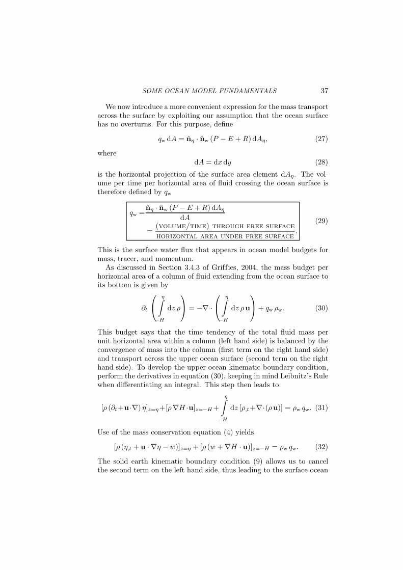
We now introduce a more convenient expression for the mass transportacross the surface by exploiting our assumption that the ocean surfacehas no overturns. For this purpose, define
qw dA = nη · nw (P − E + R) dAη, (27)
wheredA = dxdy (28)
is the horizontal projection of the surface area element dAη. The vol-ume per time per horizontal area of fluid crossing the ocean surface istherefore defined by qw
qw =nη · nw (P − E + R) dAη
dA
=(volume/time) through free surface
horizontal area under free surface.
(29)
This is the surface water flux that appears in ocean model budgets formass, tracer, and momentum.
As discussed in Section 3.4.3 of Griffies, 2004, the mass budget perhorizontal area of a column of fluid extending from the ocean surface toits bottom is given by
∂t
η∫
−H
dz ρ
= −∇ ·
η∫
−H
dz ρu
+ qw ρw. (30)
This budget says that the time tendency of the total fluid mass perunit horizontal area within a column (left hand side) is balanced by theconvergence of mass into the column (first term on the right hand side)and transport across the upper ocean surface (second term on the righthand side). To develop the upper ocean kinematic boundary condition,perform the derivatives in equation (30), keeping in mind Leibnitz’s Rulewhen differentiating an integral. This step then leads to
[ρ (∂t+u·∇) η]z=η+[ρ∇H ·u]z=−H +
η∫
−H
dz [ρ,t+∇·(ρu)] = ρw qw. (31)
Use of the mass conservation equation (4) yields
[ρ (η,t + u · ∇η − w)]z=η + [ρ (w + ∇H · u)]z=−H = ρw qw. (32)
The solid earth kinematic boundary condition (9) allows us to cancelthe second term on the left hand side, thus leading to the surface ocean

38 STEPHEN GRIFFIES
kinematic boundary condition
ρ (∂t + u · ∇) η = ρw qw + ρw at z = η (33)
which can be written in the material form
ρ
(
d(z − η)
dt
)
= −ρw qw at z = η. (34)
Contrary to the solid earth condition (10), where z + H is materiallyconstant, permeability of the ocean surface leads to a nontrivial materialevolution of z − η.
To derive the analogous s-coordinate boundary condition, we proceedas for the bottom. Here, the coordinate transformation is time depen-dent
(x, y, z, t) = (x, y, η(x, y, t), t). (35)
The horizontal gradient and time derivative operators are therefore re-lated by
∇z = ∇z + (∇ η) ∂z (36)
∂t = ∂t + η,t ∂z. (37)
Hence, the relation (16) between vertical velocity components takes thefollowing form at the ocean surface
w = z,s (d/dt − ∂t − u · ∇z) s + (∂t + u · ∇)η at z = η. (38)
Substitution of the z-coordinate kinematic boundary condition (33) leadsto
ρ z,s (d/dt − ∂t − u · ∇z) s = −ρw qw at s = stop (39)
where stop = s(x, y, z = η, t) is the value of the generalized verticalcoordinate at the ocean surface. Reorganizing the result (39) leads tothe material time derivative form
ρ z,s
(
d(s − stop)
dt
)
= −ρw qw at s = stop (40)
which is analogous to the z-coordinate result (34). Indeed, it can bederived trivially by noting that dz/dt = z,s ds/dt. Even so, it is usefulto have gone through the previous manipulations in order to garnerexperience and confidence with the formalism. Such confidence becomesof particular use in the next section focusing on the dia-surface flux.

SOME OCEAN MODEL FUNDAMENTALS 39
2.5 Dia-surface transport
We seek an expression for the flux of fluid passing through a surface ofconstant generalized vertical coordinate. The result will be an expressionfor the dia-surface transport. It plays a fundamental role in generalizedvertical coordinate modelling. Our derivation here follows that given inSection 6.7 of Griffies, 2004.
At an arbitrary point on a surface of constant generalized verticalcoordinate (see Figure 5), the flux of fluid in the direction normal to thesurface is given by
seawater flux in direction n = v · n, (41)
with
n = ∇s |∇s|−1 (42)
the surface unit normal direction. Introducing the material time deriva-tive ds/dt = s,t + v · ∇s leads to the equivalent expression
v · n = |∇s|−1 (d/dt − ∂t) s. (43)
That is, the normal component to a fluid parcel’s velocity is proportionalto the difference between the material time derivative of the surface andits partial time derivative.
Since the surface is generally moving, the net flux of seawater pene-trating the surface is obtained by subtracting the velocity of the surfacev(ref) in the n direction from the velocity component v · n of the fluidparcels
flux of seawater through surface = n · (v − v(ref)). (44)
The velocity v(ref) is the velocity of a reference point fixed on the surface,and it is written
v(ref) = u(ref) + w(ref) z. (45)
Since the reference point remains on the same s = const surface, ds/dt =0 for the reference point. Consequently, we can write the vertical velocitycomponent w(ref) as
w(ref) = −z,s (∂t + u(ref) · ∇z) s, (46)
where equation (16) was used with ds/dt = 0. This result then leads to
n · v(ref) = n · u(ref) + n · zw(ref)
= −s,t |∇s|−1,(47)

40 STEPHEN GRIFFIES
which says that the normal component of the surface’s velocity vanisheswhen the surface is static, as may be expected. It then leads to thefollowing expression for the net flux of seawater crossing the surface
n · (v − v(ref)) = |∇s|−1 (∂t + v · ∇) s
= |∇s|−1 ds/dt.(48)
Hence, the material time derivative of the generalized surface vanishesif and only if no water parcels cross it. This important result is usedthroughout ocean theory and modelling.
z
n
s=constant
vvref
x,y
Figure 5. Surfaces of constant generalized vertical coordinate living interior to theocean. An upward normal direction n is indicated on one of the surfaces. Also shownis the orientation of a fluid parcel’s velocity v and the velocity v(ref) of a referencepoint living on the surface.
Expression (48) gives the volume of seawater crossing a generalizedsurface, per time, per area. The area normalizing the volume flux is thatarea dA(n) of an infinitesimal patch on the surface of constant generalizedvertical coordinate with outward unit normal n. This area can be written(see equation (6.58) of Griffies, 2004)
dA(n) = |z,s ∇s|dxdy. (49)
Hence, the volume per time of fluid passing through the generalizedsurface is
(volume/time) through surface = n · (v − v(ref)) dA(n)
= |z,s| (ds/dt) dxdy,(50)
and the magnitude of this flux is
|n · (v − v(ref)) dA(n)| ≡ |w(s)|dxdy. (51)

SOME OCEAN MODEL FUNDAMENTALS 41
We introduced the expression
w(s) = z,s ds/dt, (52)
which measures the volume of fluid passing through the surface, perunit area dA = dxdy of the horizontal projection of the surface, perunit time. That is,
w(s) ≡n · (v − v(ref)) dA(n)
dA
=(volume/time) of fluid through surface
area of horizontal projection of surface.
(53)
The quantity w(s) is called the dia-surface velocity component. It isdirectly analogous to the fresh water flux qw defined in equation (27),which measures the volume of freshwater crossing the ocean surface,per unit time per horizontal area. To gain some experience with thedia-surface velocity component, it is useful to write it in the equivalentforms
w(s) = z,s ds/dt
= z,s ∇s · (v − v(ref))
= (z − S) · (v − v(ref))
(54)
where
S = ∇sz
= −z,s ∇zs(55)
is the slope of the s surface as projected onto the horizontal directions.For example, if the slope vanishes, then the dia-surface velocity compo-nent measures the flux of fluid moving vertically relative to the motionof the generalized surface. When the surface is static and flat, then thedia-surface velocity component is simply the vertical velocity componentw = dz/dt.
The expression (52) for w(s) allows one to write the material timederivative in one of the following equivalent manners
d
dt=
(
∂
∂t
)
z
+ u · ∇z + w
(
∂
∂z
)
=
(
∂
∂t
)
s
+ u · ∇s +ds
dt
(
∂
∂s
)
=
(
∂
∂t
)
s
+ u · ∇s + w(s)
(
∂
∂z
)
,
(56)

42 STEPHEN GRIFFIES
where ∂s = z,s ∂z. The last form motivates some to consider w(s) as avertical velocity component that measures the rate at which fluid parcelspenetrate the surface of constant generalized coordinate (see AppendixA to McDougall, 1995). One should be mindful, however, to distinguishw(s) from the generally different vertical velocity component w = dz/dt,which measures the water flux crossing constant geopotential surfaces.
We close with a few points of clarification for the case where no fluidparcels cross the generalized surface. Such occurs, in particular, in thecase of adiabatic flows with s = ρ an isopycnal coordinate. In this case,the material time derivative (56) only has a horizontal two-dimensionaladvective component u · ∇s. This result should not be interpreted tomean that the velocity of a fluid parcel is strictly horizontal. Indeed, itgenerally is not, as the previous derivation should make clear. Rather,it means that the transport of fluid properties occurs along surfacesof constant s, and such transport is measured by the convergence ofhorizontal advective fluxes as measured along surfaces of constant s.We revisit this point in Section 3.2 when discussing tracer transport(see in particular Figure 7).
3. Mass and tracer budgets
The purpose of this section is to extend the kinematics discussed inthe previous section to the case of mass and tracer budgets for finitedomains within the ocean fluid. In the formulation of ocean models,these domains are thought of as discrete model grid cells.
3.1 General formulation
Assume that mass and tracer are altered within a finite region bytransport across boundaries of the region and by sources within theregion. Hence, the tracer mass within an arbitrary fluid region evolvesaccording to
∂t
(∫∫∫
C ρdV
)
=
∫∫∫
S(C) ρdV −
∫∫
dA(n) n · [(v− vref) ρC + J].
(57)The left hand side of this equation is the time tendency for the tracermass within the region, where C is the tracer concentration and ρ isthe in situ fluid density (mass of seawater per volume). As discussedin Sections 5.1 and 5.6 of Griffies, 2004, C represents a mass of tracerper mass of seawater for non-thermodynamic tracers such as salt orbiogeochemical tracers, whereas C represents the potential temperatureor the conservative temperature (McDougall, 2003) for the “heat” tracer

SOME OCEAN MODEL FUNDAMENTALS 43
used in the model. On the right hand side, S(C) represents a tracersource with units of tracer concentration per time. As seen in Section2.5, dA(n) n ·(v−vref) measures the volume per time of fluid penetratingthe domain boundary at a point.
The tracer flux J arises from subgrid scale transport, such as diffusionand/or unresolved advection. This flux is assumed to vanish when thetracer concentration is uniform, in which case the tracer budget (57)reduces to a mass budget. In addition to the tracer flux, it is convenientto define the tracer concentration flux F via
J = ρF, (58)
where the dimensions of F are velocity × tracer concentration.
3.2 Budget for an interior grid cell
Grid cell k x,y
z
s=s
s=s
k−1
k
Figure 6. Schematic of an ocean grid cell labeled by the vertical integer k. Its sidesare vertical and oriented according to x and y, and its horizontal position is fixed intime. The top and bottom surfaces are determined by constant generalized verticalcoordinates sk−1 and sk, respectively. Furthermore, the top and bottom are assumedto always have an outward normal with a nonzero component in the vertical directionz. That is, the top and bottom are never vertical. Note that we take the conventionthat the discrete vertical label k increases as moving downward in the column, andgrid cell k is bounded at its upper face by s = sk−1 and lower face by s = sk.
Consider the budget for a region bounded away from the ocean surfaceand bottom, such as that shown in Figure 6. There are two assumptionswhich define a grid cell region in this case.
The sides of the cell are vertical, and so they are parallel to z
and aligned with the horizontal coordinate directions (x, y). Theirhorizontal positions are fixed in time.

44 STEPHEN GRIFFIES
The top and bottom of the cell are defined by surfaces of constantgeneralized vertical coordinate s = s(x, y, z, t). The generalizedsurfaces do not overturn, which means that s,z is single signedthroughout the ocean.
These assumptions lead to the following results for the sides of the gridcell
tracer mass entering cell west face =
∫∫
x=x1
dy dz (u ρC + ρF x) (59)
tracer mass leaving cell east face = −
∫∫
x=x2
dy dz (u ρC + ρF x) (60)
where x1 ≤ x ≤ x2 defines the domain boundaries for the east-westcoordinates.8 Similar results hold for the tracer mass crossing the cellin the north-south directions. At the top and bottom of the grid cell9
tracer mass entering cell bottom face =
∫∫
s=sk
dxdy ρ (w(s) C + F (s)) (61)
tracer mass leaving cell top face = −
∫∫
s=sk−1
dxdy ρ (w(s) C + F (s)). (62)
To reach this result, we used a result from Section 2.5 to write the volumeflux passing through the top face of the grid cell
dA(n) n · (v − vref) = w(s) dxdy, (63)
with w(s) = z,s ds/dt the dia-surface velocity component. A similarrelation holds for the bottom face of the cell. The form of the SGS fluxpassing across the top and bottom is correspondingly given by
dA(n) n · J = J (s) dxdy. (64)
Since the model is using the generalized coordinate s for the vertical,it is convenient to do the vertical integrals over s instead of z. For this
8We use generalized horizontal coordinates, such as those discussed in Griffies, 2004. Hence,the directions east, west, north, and south may not correspond to the usual geographicdirections. Nonetheless, this terminology is useful for establishing the budgets, whose validityis general.9As seen in Section 6, for pressure-like vertical coordinates, s increases with depth. Fordepth-like vertical coordinates, s decreases with depth. It is important to keep this signdifference in mind when formulating the budgets in the various coordinates. Notably, thespecific thickness z,s carries the sign.

SOME OCEAN MODEL FUNDAMENTALS 45
purpose, recall that with z,s single signed, the vertical thickness of a gridcell is
dz = z,s ds. (65)
Bringing these results together, and taking the limit as the volume ofthe cell in (x, y, s) space goes to zero (i.e., dxdy ds → 0) leads to
∂t(z,s ρC) = z,s ρS(C)−∇s · [z,s ρ (uC +F)]−∂s [ ρ (w(s) C+F (s))] (66)
Notably, the horizontal gradient operator ∇s is computed on surfaces ofconstant s, and so it is distinct generally from the horizontal gradient ∇z
taken on surfaces of constant z. Instead of taking the limit as dxdy ds →0, it convenient for discretization purposes to take the limit as the timeindependent horizontal area dxdy goes to zero, thus maintaining thetime dependent thickness dz = z,s ds inside the derivative operators. Inthis case, the thickness weighted tracer mass budget takes the form
∂t(dz ρC) = dz ρS(C) −∇s · [dz ρ (uC + F)]
− [ρ (w(s) C + F (s))]s=sk−1+ [ρ (w(s) C + F (s))]s=sk
.
(67)Similarly, the thickness weighted mass budget is
∂t(dz ρ) = dz ρS(M) −∇s · (dz ρu)
− (ρw(s))s=sk−1+ (ρw(s))s=sk
.(68)
where S(M) is a mass source with units of inverse time that is related tothe tracer source via
S(M) = S(C)(C = 1), (69)
and the SGS flux vanishes with a uniform tracer
F(C = 1) = 0. (70)
3.3 Budgets without dia-surface fluxes
To garner some experience with these budgets, it is useful to considerthe special case of zero dia-surface transport, either via advection orSGS fluxes, and zero tracer/mass sources. In this case, the thicknessweighted mass and tracer mass budgets take the simplified form
∂t(dz ρ) = −∇s · (dz ρu) (71)
∂t(dz ρC) = −∇s · [dz ρ (uC + F)]. (72)
The first equation says that the time tendency of the thickness weighteddensity (mass per area) at a point between two surfaces of constant

46 STEPHEN GRIFFIES
generalized vertical coordinate is given by the horizontal convergence ofmass per area onto that point. The transport is quasi-two-dimensional inthe sense that it is only a two-dimensional convergence that determinesthe evolution. The tracer equation has an analogous interpretation. Weillustrate this situation in Figure 7. As emphasized in our discussionof the material time derivative (56), this simplification of the transportequation does not mean that fluid parcels are strictly horizontal. Indeed,such is distinctly not the case when the surfaces are moving.
A further simplification of the mass and tracer mass budgets ensueswhen considering adiabatic and Boussinesq flow in isopycnal coordinates.We consider ρ now to represent the constant potential density of thefinitely thick fluid layer. In this case, the mass and tracer budgets reduceto
∂t(dz) = −∇ρ · (dz u) (73)
∂t(dz C) = −∇ρ · [dz (uC + F)]. (74)
Equation (73) provides a relation for the thickness of the density layers,and equation (74) is the analogous relation for the tracer within the layer.These expressions are commonly used in the construction of adiabaticisopycnal models, which are often used in the study of geophysical fluidmechanics of the ocean.
k−1diverge
converge converge
s=sk
s=s
Figure 7. Schematic of the horizontal convergence of mass between two surfaces ofconstant generalized vertical coordinates. As indicated by equation (71), when thereis zero dia-surface transport, it is just the horizontal convergence that determines thetime evolution of mass between the layers. Evolution of thickness weighted tracerconcentration in between the layers is likewise evolved just by the horizontal conver-gence of the thickness weighted advective and diffusive tracer fluxes (equation (72)).In this way, the transport is quasi-two-dimensional when the dia-surface transportsvanish. A common example of this special system is an adiabatic ocean where thegeneralized surfaces are defined by isopycnals.
3.4 Cells adjacent to the ocean bottom
For a grid cell adjacent to the ocean bottom (Figure 8), we assumethat just the bottom face of this cell abuts the solid earth boundary.The outward normal nH to the bottom is given by equation (7), and the

SOME OCEAN MODEL FUNDAMENTALS 47
z=−H
x,y
z
s=skbot−1
Grid cell k=kbot
bots=s
Figure 8. Schematic of an ocean grid cell next to the ocean bottom labeled by k =kbot. Its top face is a surface of constant generalized vertical coordinate s = skbot−1,and the bottom face is determined by the ocean bottom topography at z = −H wheresbot(x, y, t) = s(x, y, z = −H, t).
area element along the bottom is
dAH = |∇(z + H)|dxdy. (75)
Hence, the transport across the solid earth boundary is
−
∫∫
dAH nH · (v ρC + J) =
∫∫
dxdy (∇H + z) · (v ρC + J). (76)
We assume that there is zero mass flux across the bottom, in whichcase the advective flux drops out since v · (∇H + z) = 0 (equation(9)). However, the possibility of a nonzero geothermal tracer transportwarrants a nonzero SGS tracer flux at the bottom, in which case thebottom tracer flux is written
Q(C)(bot) = (∇H + z) · J. (77)
The corresponding thickness weighted budget is given by
∂t (dz ρC) = dz ρS(C) −∇s · [dz ρ (uC + F)]
−[
ρ (w(s) C + z,s ∇s · F)]
s=skbot−1
+ Q(C)(bot),
(78)
and the corresponding mass budget is
∂t (dz ρ) = dz ρS(M) −∇s · (dz ρu) − (ρws))s=skbot−1. (79)

48 STEPHEN GRIFFIES
3.5 Cells adjacent to the ocean surface
Grid cell k=1
x,y
z
z=−H
s=sk=1
s=stop z=η
Figure 9. Schematic of an ocean grid cell next to the ocean surface labeled by k = 1.Its top face is at z = η, and the bottom is a surface of constant generalized verticalcoordinate s = sk=1.
For a grid cell adjacent to the ocean surface (Figure 9), we assumethat just the upper face of this cell abuts the boundary between theocean and the atmosphere or sea ice. The ocean surface is a time de-pendent boundary with z = η(x, y, t). The outward normal nη is givenby equation (25), and its area element dAη is given by equation (26).
As the surface can move, we must measure the advective transportwith respect to the moving surface. Just as in the dia-surface transportdiscussed in Section 2.5, we consider the velocity of a reference point onthe surface
vref = uref + zwref. (80)
Since z = η represents the vertical position of the reference point, thevertical component of the velocity for this point is given by
wref = (∂t + uref · ∇) η (81)
which then leads tovref · ∇ (z − η) = η,t. (82)
Hence, the advective transport leaving the ocean surface is∫∫
z=η
dA(n) n · (v − vref) ρC =
∫∫
z=η
dxdy (−η,t + w − u · ∇η) ρC
= −
∫∫
z=η
dxdy ρw qw C,
(83)

SOME OCEAN MODEL FUNDAMENTALS 49
where the surface kinematic boundary condition (33) was used. Thenegative sign on the right hand side arises from our convention thatqw > 0 represents an input of water to the ocean domain. In summary,the tracer flux leaving the ocean free surface is given by
∫∫
z=η
dA(n) n · [(v − vref) ρC + J] =
∫∫
z=η
dxdy (−ρw qw C + ∇ (z − η) · J).
(84)In the above, we formally require the tracer concentration precisely
at the ocean surface z = η. However, as mentioned at the start ofSection 2.4, it is actually a fiction that the ocean surface is a smoothmathematical function. Furthermore, seawater properties precisely atthe ocean surface, known generally as skin properties, are generally notwhat an ocean model carries as its prognostic variable in its top grid cell.Instead, the model carries a bulk property averaged over roughly theupper few tens of centimeters. The lectures at this school by ProfessorIan Robinson discuss these important points in the context of measuringsea surface temperature from a satellite, where the satellite measures theskin temperature, not the foundational or bulk temperature carried bylarge-scale ocean models.
To proceed in formulating the boundary condition for an ocean climatemodel, whose grid cells we assume to be at least a meter in thickness,we consider there to be a boundary layer model that provides us withthe total tracer flux passing through the ocean surface. Developing sucha model is a nontrivial problem in air-sea and ice-sea interaction theoryand phenomenology. For present purposes, we do not focus on thesedetails, and instead just introduce this flux in the form
Q(C) = −ρw qw Cw + Q(C)(turb) (85)
where Cw is the tracer concentration in fresh water. The first term repre-sents the advective transport of tracer through the surface with the fresh
water (i.e., ice melt, rivers, precipitation, evaporation). The term Q(C)(turb)
arises from parameterized turbulence and/or radiative fluxes, such assensible, latent, shortwave, and longwave heating appropriate for the
temperature equation. A positive value for Q(C)(turb) signals tracer leaving
the ocean through its surface. In the special case of zero fresh waterflux, then
∇ (z − η) · J = Q(C)(turb) if qw = 0. (86)

50 STEPHEN GRIFFIES
In general, it is not possible to make this identification. Instead, wemust settle for the general expression∫∫
z=η
dA(n) n · [(v−vref) ρC +J] =
∫∫
z=η
dxdy (−ρw qw Cw +Q(C)(turb)). (87)
The above results lead to the thickness weighted tracer budget for theocean surface grid cell
∂t (dz ρC) = dz ρS(C) −∇s · [dz ρ (uC + F)]
+[
ρ (w(s) C + z,s ∇s ·F)]
s=sk=1
+ (ρw qw Cw − Q(turb)(C)
),
(88)
and the corresponding mass budget
∂t (dz ρ) = dz ρS(M) −∇s · (dz ρu) + (ρw(s))s=sk=1+ ρw qw. (89)
3.6 Surface boundary condition for salt
We close this section by mentioning the free ocean surface boundarycondition for salt and other material tracers. Salt is transferred intothe ocean with brackish river water and ice melt of nonzero salinity.Yet evaporation and precipitation generally leave the salt content of theocean unchanged. In these latter cases, the boundary layer tracer flux(85) vanishes
Q(salt) = 0. (90)
This trivial boundary condition is also appropriate for many other ma-terial tracers, such as those encountered with ocean biogeochemical pro-cesses. In these cases, the tracer concentration is not altered via thepassage of tracer across the surface. Instead, it is altered via the trans-port of fresh water across the ocean free surface which acts to dilute orconcentrate the tracer.
The boundary condition (90) is often replaced in ocean models by avirtual tracer flux condition, whereby tracer is transferred into the modelin lieu of altering the ocean water mass via the transport of fresh wa-ter. Virtual tracer flux boundary conditions are required for rigid lidmodels (Bryan, 1969) that maintain a constant volume and so cannotincorporate surface fresh water fluxes. However, there remain few rigidlid models in use today, and there is no reason to maintain the virtualtracer flux in the more commonly used free surface models. The dif-ferences in solution may be minor for many purposes, especially short

SOME OCEAN MODEL FUNDAMENTALS 51
integrations (e.g., less than a year). However, the feedbacks related toclimate and climate change may be nontrivial. Furthermore, the changesin model formulation are minor once a free surface algorithm has beenimplemented. Thus, it is prudent and straightforward to jettison the vir-tual tracer flux in favor of the physically motivated boundary condition(90) (Huang, 1993 and Griffies et al., 2001).
4. Linear momentum budget
The purpose of this section is to formulate the budget for linear mo-mentum over a finite region of the ocean, with specific application toocean model grid cells. The material here requires many of the sameelements as in Section 3, but with added complexity arising from thevector nature of momentum, and the additional considerations of forcesfrom pressure, friction, gravity, and planetary rotation.
4.1 General formulation
The budget of linear momentum for a finite region of fluid is given bythe following relation based on Newton’s second and third laws
∂t
(∫∫∫
dV ρv
)
= −
∫∫
dA(n) [ n · (v − vref)] ρv
+
∫∫
dA(n) (n · τ − n p)
−
∫∫∫
dV ρ [ g z + (f + M) z ∧ v].
(91)
The left hand side is the time tendency of the region’s linear momentum.The first term on the right hand side is the advective transport of linearmomentum across the boundary of the region, with recognition that theregion’s boundaries are generally moving with velocity vref. The secondterm is the integral of the contact stresses due to friction and pressure.These stresses act on the boundary of the fluid domain. The stress tensorτ is a symmetric second order tensor that parameterizes subgrid scaletransport of momentum. The final term on the right hand side is thevolume integral of body forces due to gravity and the Coriolis force.10 Inaddition, there is a body force arising from the nonzero curvature of thespherical space. This curvature leads to the advection metric frequency(see equation (4.49) of Griffies, 2004) M = v ∂x ln dy − u∂y ln dx. The
10The wedge symbol ∧ represents a vector cross product, also commonly written as ×. Thewedge is typically used in the physics literature, and is preferred here to avoid confusion withthe horizontal coordinate x.

52 STEPHEN GRIFFIES
advection metric frequency arises since linear momentum is not con-served on the sphere.11 Hence, the linear momentum budget picks upthis extra term that is a function of the chosen lateral coordinates. Theadvection metric frequency is analogous to, but far smaller than, theCoriolis frequency.
Unlike the case of the tracer and mass balances considered in Section3, we do not consider momentum sources interior to the fluid domain.Such may be of interest and can be introduced without difficulty. Thegoal of the remainder of this section is to consider the linear momentumbalance for finite grid cells in an ocean model.
4.2 An interior grid cell
At the west side of a grid cell, n = −x whereas n = x on the east side.Hence, the advective transport of linear momentum entering through thewest side of the grid cell and that which is leaving through the east sideare given by
transport entering from west =
∫∫
x=x1
dy ds z,s u (ρv) (92)
transport leaving through east = −
∫∫
x=x2
dy ds z,s u (ρv). (93)
Similar results hold for momentum crossing the cell boundaries in thenorth and south directions. Momentum crossing the top and bottomsurfaces of an interior cell is given by
transport entering from the bottom =
∫∫
s=s2
dxdy w(s) (ρv) (94)
transport leaving from the top = −
∫∫
s=s1
dxdy w(s) (ρv). (95)
11Angular momentum is conserved for frictionless flow on the sphere in the absence of hori-zontal boundaries (see Section 4.11.2 of Griffies, 2004).
SOME OCEAN MODEL FUNDAMENTALS 53
Forces due to the contact stresses at the west and east sides are givenby
contact force on west side = −
∫∫
x=x1
dy ds z,s (x · τ − x p) (96)
contact force on east side =
∫∫
x=x2
dy ds z,s (x · τ − x p) (97)
with similar results at the north and south sides. At the top of thecell, dA(n) n = ∇s dxdy whereas dA(n) n = −∇s dxdy at the bottom.Hence,
contact force on cell top =
∫∫
s=sk−1
dxdy z,s (∇s · τ − p∇s) (98)
contact force on cell bottom = −
∫∫
s=sk
dy ds z,s (∇s · τ − p∇s). (99)
Bringing these results together, and taking limit as the time independenthorizontal area dxdy → 0, leads to the thickness weighted budget forthe momentum per horizontal area of an interior grid cell
∂t (dz ρv) = −∇s · [ dz u (ρv)]
+ (w(s) ρv)s=sk− (w(s) ρv)s=sk−1
+ ∂x [ dz (x · τ − x p)]
+ ∂y [ dz (y · τ − y p)]
+ [z,s (∇s · τ − p∇s)]s=sk−1
− [z,s (∇s · τ − p∇s)]s=sk
− ρdz [ g z + (f + M) z ∧ v].
(100)
Note that both the time and horizontal partial derivatives are for po-sitions fixed on a constant generalized vertical coordinate surface. Ad-ditionally, we have yet to take the hydrostatic approximation, so theseequations are written for the three components of the vertical velocity.
The first term on the right hand side of the thickness weighted mo-mentum budget (100) is the convergence of advective momentum fluxesoccurring within the layer. We discussed the analogous flux conver-gence for the tracer and mass budgets in Section 3.3. The second andthird terms arise from the transport of momentum across the upper andlower constant s interfaces. The fourth and fifth terms arise from the

54 STEPHEN GRIFFIES
horizontal convergence of pressure and viscous stresses. The sixth andseventh terms arise from the frictional and pressure stresses acting onthe constant generalized surfaces. These forces provide an interfacialstress between layers of constant s. Note that even in the absence offrictional stresses, interfacial stresses from pressure acting on the gener-ally curved s surface can transmit momentum between vertically stackedlayers. The final term arises from the gravitational force, the Coriolisforce, and the advective frequency.
4.3 Cell adjacent to the ocean bottom
As for the tracer and mass budgets, we assume zero mass flux throughthe ocean bottom at z = −H(x, y). However, there is generally a nonzerostress at the bottom due to both the pressure between the fluid and thebottom, and unresolved features in the flow which can correlate or anti-correlate with bottom topographic features (Holloway, 1999). The areaintegral of the stresses lead to a force on the fluid at the bottom
Fbottom = −
∫∫
z=−H
dxdy [∇(z + H) · τ − p∇(z + H)]. (101)
Details of the stress term requires fine scale information that is generallyunavailable. For present purposes we assume that some boundary layermodel provides information that is schematically written
τbot = ∇(z + H) · τ (102)
where τbot is a vector bottom stress. Taking the limit as the horizontal
area vanishes leads to the thickness weighted budget for momentum perhorizontal area of a grid cell next to the ocean bottom
∂t (dz ρv) = −∇s · [ dz u (ρv)] − (w(s) ρv)s=skbot−1
+ ∂x [ dz (x · τ − x p)]
+ ∂y [ dz (y · τ − y p)]
+ [z,s (∇s · τ − p∇s)]s=skbot−1
− τbot + pb ∇(z + H)
− ρdz [ g z + (f + M) z ∧ v].
(103)
4.4 Cell adjacent to the ocean surface
There is a nonzero mass and momentum flux through the upper oceansurface at z = η(x, y, t), and contact stresses are applied from resolvedand unresolved processes involving interactions with the atmosphere and

SOME OCEAN MODEL FUNDAMENTALS 55
sea ice. Following the discussion of the tracer budget at the ocean surfacein Section 3.5 leads to the expression for the transport of momentum intothe ocean due to mass transport at the surface
−
∫∫
dA(n) n · [(v − vref) ρv =
∫∫
z=η
dxdy ρw qw v. (104)
The force arising from the contact stresses at the surface is written
Fcontact =
∫∫
z=η
dxdy [∇ (z − η) · τ − p∇ (z − η)]. (105)
Bringing these results together leads to the force acting at the oceansurface
Fsurface =
∫∫
z=η
dxdy [∇ (z − η) · τ − p∇ (z − η) + ρw qw v]. (106)
Details of the various terms in this force are generally unknown. There-fore, just as for the tracer at z = η in Section 3.5, we assume that aboundary layer model provides information about the total force, andthat this force is written
Fsurface =
∫∫
z=η
dxdy [ τ top − pa ∇ (z − η) + ρw qw vw], (107)
where vw is the velocity of the fresh water. This velocity is typicallytaken to be equal to the velocity of the ocean currents in the top cellsof the ocean model, but such is not necessarily the case when consid-ering the different velocities of, say, river water and precipitation. Thestress τ
top is that arising from the wind, as well as interactions betweenthe ocean and sea ice. Letting the horizontal area vanish leads to thethickness weighted budget for a grid cell next to the ocean surface
∂t (dz ρv) = −∇s · [ dz u (ρv)] + (w(s) ρv)s=sk=1
+ ∂x [ dz (x · τ − x p)]
+ ∂y [ dz (y · τ − y p)]
− [z,s (∇s · τ − p∇s)]s=sk=1
+ [ τ top − pa ∇ (z − η) + ρw qw vw]
− ρdz [ g z + (f + M) z ∧ v].
(108)

56 STEPHEN GRIFFIES
5. The pressure force
A hydrostatic fluid maintains the balance p,z = −ρ g. This balancemeans that the pressure at a point in a hydrostatic fluid is determinedby the weight of fluid above this point. This relation is maintained quitewell in the ocean on spatial scales larger than roughly 1km. Precisely,when the squared ratio of the vertical to horizontal scales of motion issmall, then the hydrostatic approximation is well maintained. In thiscase, the vertical momentum budget reduces to the hydrostatic balance,in which case vertical acceleration and friction are neglected. If we areinterested in explicitly representing such motions as Kelvin-Helmholtzbillows and flow within a convective chimney, vertical accelerations arenontrivial and so the non-hydrostatic momentum budget must be used.
The hydrostatic balance greatly affects the algorithms used to numer-ically solve the equations of motion. The paper by Marshall et al., 1997highlights these points in the context of developing an algorithm suitedfor both hydrostatic and non-hydrostatic simulations. However, so far inocean modelling, no global simulations have been run at resolutions suf-ficiently refined to require the non-hydrostatic equations. Additionally,many regional and coastal models, even some with resolutions refinedsmaller than 1km, still maintain the hydrostatic approximation, and thusthey must parameterize the unrepresented non-hydrostatic motions.
At a point in the continuum, the horizontal pressure gradient forcefor the hydrostatic and non-Boussinesq set of equations can be written12
ρ−1 ∇zp = ρ−1 (∇s −∇s z ∂z) p
= ρ−1 ∇s p + g∇s z,
= ∇s (p/ρ + g z) − p∇sρ−1
(109)
where the hydrostatic relation p,z = −ρ g was used to reach the secondequality. The term p/ρ+g z is known as the Montgomery potential. Forcases where the density term ∇sρ vanishes (such as when s is propor-tional to density), the pressure gradient force takes the form of a totalgradient, and so it has a zero curl thus facilitating the formulation ofvorticity budgets.
In general, the difficulty of numerically realizing the pressure gradi-ent force arises when there are contributions from both the Montgomerypotential and the density gradient terms in equation (109). Naive dis-cretizations result in both terms being large and of opposite sign in
12For a Boussinesq fluid, equation (109) is modified by a factor of ρ/ρo. Hence, the same issuesarise when numerically implementing the pressure gradient force with generalized verticalcoordinates in either the Boussinesq or non-Boussinesq fluids.
SOME OCEAN MODEL FUNDAMENTALS 57
many regions. Hence, they expose the calculation to nontrivial numeri-cal truncation errors which can lead to spurious pressure gradients thatspin up an unforced fluid with initially flat isopycnals. Significant efforthas gone into reducing such pressure gradient errors, especially in ter-rain following models where undulations of the coordinate surfaces canbe large with realistic bottom topography (e.g., see Figure 12). Someof these issues are summarized, with references, in Section 2 of Griffieset al., 2000a. Perhaps the most promising approach is that proposedby Shchepetkin and McWilliams, 2002. It is notable that difficultieswith pressure gradient errors have largely been responsible for the nearabsence of sigma models being used for long term global ocean climatesimulations.13
6. Elements of vertical coordinates
As discussed in Griffies et al., 2000a, there are broadly three regimesof the ocean germane to the considerations of a vertical coordinate.
Upper ocean mixed layer: This is a generally turbulent regiondominated by transfers of momentum, heat, freshwater, and trac-ers with the overlying atmosphere, sea ice, rivers, etc. It is of primeimportance for climate system modelling and operational oceanog-raphy. It is typically very well mixed in the vertical through three-dimensional convective/turbulent processes. These processes in-volve non-hydrostatic physics which requires very high horizontaland vertical resolution (i.e., a vertical to horizontal grid aspect ra-tio near unity) to explicitly represent. A parameterization of theseprocesses is therefore necessary in primitive equation ocean mod-els. In this region, it is essential to employ a vertical coordinatethat facilitates the representation and parameterization of thesehighly turbulent processes. Geopotential and pressure coordinates,or their relatives, are the most commonly used coordinates as theyfacilitate the use of very refined vertical grid spacing, which canbe essential to simulate the strong exchanges between the oceanand atmosphere, rivers, and ice.
Ocean interior: Tracer transport processes in the ocean interiorpredominantly occur along neutral directions (McDougall, 1987).The transport is dominated by large scale currents and mesoscaleeddy fluctuations. Water mass properties in the interior thus tend
13The work of Diansky et al., 2002 is the only case known by the author of a global sigmamodel used for climate purposes.

58 STEPHEN GRIFFIES
to be preserved over large space and time scales (e.g., basin anddecade scales). This property of the ocean interior is critical to rep-resent in a numerical simulation of ocean climate. An isopycnalcoordinate framework is well suited to this task, whereas geopo-tential and sigma models have problems associated with numericaltruncation errors. As discussed by Griffies et al., 2000b, the prob-lem becomes more egregious as the model resolution is refined, dueto the enhanced levels of eddy activity that pumps tracer varianceto the grid scale. Quasi-adiabatic dissipation of this variance isdifficult to maintain in non-isopycnal models.
Ocean bottom: The solid earth bottom topography directly influ-ences the overlying currents. In an unstratified ocean, the balancedflow generally follows lines of constant f/H, where f is the Corio-lis parameter and H ocean depth. Additionally, there are severalregions where density driven currents (overflows) and turbulentbottom boundary layer (BBL) processes act as a strong determi-nant of water mass characteristics. Many such processes are crucialfor the formation of deep water properties in the World Ocean, andfor representing coastal processes in regional models. It is for thisreason that sigma models have been developed over the past fewdecades, with their dominant application focused on the coastaland estuarine problem.
These three regimes impact on the design of vertical coordinates forocean models. In this section, we detail some vertical coordinates andsummarize their strengths and weaknesses, keeping in mind the abovephysical considerations.
6.1 Depth based vertical coordinates
We use depth based vertical coordinates in this section to discretizethe Boussinesq equations.14 Depth based coordinates are also known asvolume based coordinates, since for a Boussinesq model which uses depthas the vertical coordinate, the volume of interior grid cells is constantin the absence of sources. Correspondingly, depth based coordinates arenaturally suited for Boussinesq fluids.
14Greatbatch and McDougall, 2003 discuss an algorithm for non-Boussinesq dynamics in az-model. Their methods are implemented in the MOM4 code of Griffies et al., 2004. Thisapproach may be of special use for non-Boussinesq non-hydrostatic z-models. However, whenfocusing on hydrostatic models as we do here, pressure based vertical coordinates discussedin Section 6.2 are more convenient.

SOME OCEAN MODEL FUNDAMENTALS 59
The equations describing a Boussinesq fluid are derived from the non-Boussinesq set derived in Sections 3 and 4 by replacing all appearancesof in situ density ρ by a constant density ρo, except when density is usedto compute the buoyancy forces arising from gravity. The density ρo isa representative density of the ocean fluid, such as ρo = 1035 kg m−3.For much of the ocean, the in situ density varies less than 2% from thisvalue (see page 47 of Gill, 1982).
Depth coordinate. With a free surface, the vertical domain overwhich the z-coordinate s = z ranges is given by the time dependentinterval −H ≤ z ≤ η. Consequently, the sum of the vertical grid cellincrements equals to the total depth of the column
∑
k dz = H +η. Thetrivial specific thickness z,s = 1 simplifies the Boussinesq budgets.
The depth coordinate is useful for many purposes in global climatemodelling, and models based on depth are the most popular ocean cli-mate models. Their advantages include the following.
Simple numerical methods have been successfully used in this frame-work.
The horizontal pressure gradient can be easily represented in anaccurate manner.
The equation of state for ocean water can be accurately representedin a straightforward manner (e.g., McDougall et al., 2003).
The upper ocean mixed layer is well parameterized using a z-coordinate.
Unfortunately, these models have some well known disadvantages, whichinclude the following.
Representation of tracer transport within the quasi-adiabatic in-terior is cumbersome, with problems becoming more egregious asmesoscale eddies are admitted (Griffies et al., 2000b).
Representation and parameterization of bottom boundary layerprocesses and flow are unnatural.
Grid cells have static vertical increments ds = dz when s = z, exceptfor the top. At the top, ∂t (dz) = η,t. The time dependent verticalrange of the coordinate slightly complicates a numerical treatment of thesurface cell in z-models (see Griffies et al., 2001 for details of one suchtreatment). More problematic, however, is the possibility of a vanishingtop grid cell. That is, the surface cell can be lost (i.e., can becomedry) if the free surface depresses below the depth of the top grid cell’s
60 STEPHEN GRIFFIES
bottom face. This is a very inconvenient feature that limits the useof z-coordinates.15 In particular, the following studies may require veryrefined vertical resolution and/or large undulations of the surface height,and so would not be accessible with a conventional free surface z-model.
Process studies of surface mixing and biological cycling may war-rant very refined upper ocean grid cell thickness, some as refinedas 1m.
Realistic tidal fluctuations in some parts of the World Ocean canreach 10m-20m.
Coastal models tend to require refined vertical resolution to rep-resent shallow coastal processes along the continental shelves andnear-shore.
When coupled to a sea ice model, the weight of the ice will depressthe ocean free surface.
An example of depth coordinates. In some of the followingdiscussion, we illustrate aspects of vertical coordinates by diagnosingvalues for the coordinates from a realistic z-model run with partial stepthicknesses. Partial steps have arbitrary thickness which are set to ac-curately represent the bottom topography. The partial step technologywas introduced by Adcroft et al., 1997 in the C-grid MITgcm, and fur-ther discussed by Pacanowski and Gnanadesikan, 1998 for the B-gridModular Ocean Model (MOM). Figure 10 compares the representationof topography in a z-model using partial steps as realized in the MOMcode of Griffies et al., 2004. Many z-models have incorporated the par-tial step technology as it provides an important facility to accuratelyrepresent flow and waves near topography.
In the representation of bottom topography, there is an artificial dis-tinction between a vertical face of a cell and its horizontal top and bot-tom faces. There is no such distinction in the real ocean. As notedin Anne Marie Treguier’s lectures at this school, the block structure oftopography in z-models has the potential to affect the level of bottomfriction. The effects on bottom friction come in by noting that for aC-grid, it is straightforward to run with free-slip side walls as well asbottom faces. In contrast, B-grids use a no-slip side wall and free slip
15Linearized free surfaces, in which the budgets for tracer and momentum are formulatedassuming a constant top cell thickness, avoid problems with vanishing top cells. However,such models do not conserve total tracer or volume in the presence of a surface fresh waterflux (see Griffies et al., 2001, Campin et al., 2004 for discussion).
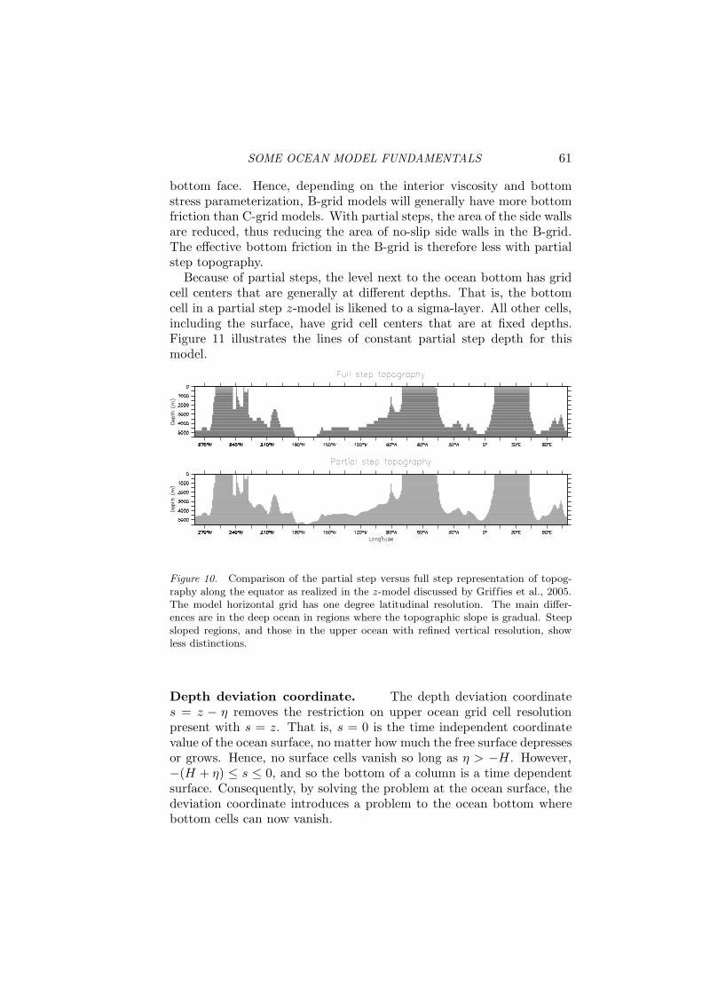
SOME OCEAN MODEL FUNDAMENTALS 61
bottom face. Hence, depending on the interior viscosity and bottomstress parameterization, B-grid models will generally have more bottomfriction than C-grid models. With partial steps, the area of the side wallsare reduced, thus reducing the area of no-slip side walls in the B-grid.The effective bottom friction in the B-grid is therefore less with partialstep topography.
Because of partial steps, the level next to the ocean bottom has gridcell centers that are generally at different depths. That is, the bottomcell in a partial step z-model is likened to a sigma-layer. All other cells,including the surface, have grid cell centers that are at fixed depths.Figure 11 illustrates the lines of constant partial step depth for thismodel.
Figure 10. Comparison of the partial step versus full step representation of topog-raphy along the equator as realized in the z-model discussed by Griffies et al., 2005.The model horizontal grid has one degree latitudinal resolution. The main differ-ences are in the deep ocean in regions where the topographic slope is gradual. Steepsloped regions, and those in the upper ocean with refined vertical resolution, showless distinctions.
Depth deviation coordinate. The depth deviation coordinates = z − η removes the restriction on upper ocean grid cell resolutionpresent with s = z. That is, s = 0 is the time independent coordinatevalue of the ocean surface, no matter how much the free surface depressesor grows. Hence, no surface cells vanish so long as η > −H. However,−(H + η) ≤ s ≤ 0, and so the bottom of a column is a time dependentsurface. Consequently, by solving the problem at the ocean surface, thedeviation coordinate introduces a problem to the ocean bottom wherebottom cells can now vanish.

62 STEPHEN GRIFFIES
Figure 11. Constant depth surfaces in a realistic ocean model. Deviations fromhorizontal next to the bottom arise from the use of partial bottom cell thicknesses,as illustrated in Figure 10. Shown here is a section along 150◦W .
Zstar coordinate. To overcome problems with vanishing surfaceand/or bottom cells, we consider the zstar coordinate
z∗ = H (z − η)/(H + η). (110)
This coordinate is closely related to the “eta” coordinate used in manyatmospheric models (see Black, 1994 for a review). It was originallyused in ocean models by Stacey et al., 1995 for studies of tides next toshelves, and it has been recently promoted by Adcroft and Campin, 2004for global climate modelling.
The surfaces of constant z∗ are quasi-horizontal. Indeed, the z∗ co-ordinate reduces to z when η is zero. In general, when noting the largedifferences between undulations of the bottom topography versus un-dulations in the surface height, it is clear that surfaces constant z∗ are

SOME OCEAN MODEL FUNDAMENTALS 63
very similar to the depth surfaces shown in Figure 11. These propertiesgreatly reduce difficulties of computing the horizontal pressure gradientrelative to terrain following sigma models discussed next. Additionally,since z∗ = z when η = 0, no flow is spontaneously generated in an un-forced ocean starting from rest, regardless the bottom topography. Thisbehavior is in contrast to the case with sigma models, where pressuregradient errors in the presence of nontrivial topographic variations cangenerate spontaneous flow from a resting state. The quasi-horizontal na-ture of the coordinate surfaces also facilitates the implementation of neu-tral physics parameterizations in z∗ models using the same techniquesas in z-models (see Chapters 13-16 of Griffies, 2004 for a discussion ofneutral physics in z-models).
The range over which z∗ varies is time independent −H ≤ z∗ ≤ 0.Hence, all cells remain nonvanishing, so long as the surface height main-tains η > −H. This is a minor constraint relative to that encounteredon the surface height when using s = z or s = z − η.
Because z∗ has a time independent range, all grid cells have staticincrements ds, and the sum of the vertical increments yields the timeindependent ocean depth
∑
k ds = H. The z∗ coordinate is thereforeinvisible to undulations of the free surface, since it moves along with thefree surface. This property means that no spurious vertical transportis induced across surfaces of constant z∗ by motion of external gravitywaves. Such spurious transport can be a problem in z-models, espe-cially those with tidal forcing. Quite generally, the time independentrange for the z∗ coordinate is a very convenient property that allowsfor a nearly arbitrary vertical resolution even in the presence of largeamplitude fluctuations of the surface height.
Depth sigma coordinate. The depth-sigma coordinate
σ = (z − η)/(H + η) (111)
is the canonical terrain following coordinate. Figure 12 illustrates thiscoordinate in a realistic model. The sigma coordinate has a long historyof use in coastal modelling. For reviews, see Greatbatch and Mellor,1999 and Ezer et al., 2002. Models based on the sigma coordinate havealso been successfully extended to basinwide studies, as well as recentglobal work by Diansky et al., 2002.
Just as for z∗ = H σ, the range over which the sigma coordinatevaries is time independent and given by −1 ≤ σ ≤ 0. Hence, all cellshave static grid increments ds, and the sum of the vertical incrementsyields unity
∑
k ds = 1. So long as the surface height is not depressed

64 STEPHEN GRIFFIES
deeper than the ocean bottom (i.e., so long as η > −H), then all cellsremain nonvanishing.16
In addition to not worrying about vanishing grid cells, some key ad-vantages of sigma models are the following.
They provide a natural framework to represent bottom influencedflow and to parameterize bottom boundary layer processes.
Thermodynamic effects associated with the equation of state arewell represented.
However, some of the disadvantages are the following:
As with the z-models, the representation of the quasi-adiabatic in-terior is cumbersome due to numerical truncation errors inducingunphysically large levels of spurious mixing, especially in the pres-ence of vigorous mesoscale eddies. Parameterization of these pro-cesses using neutral physics schemes may be more difficult numer-ically than in the z-models. The reason is that neutral directionsgenerally have slopes less than 1/100 relative to the horizontal, butcan have order unity slopes relative to sigma surfaces. The largerrelative slopes precludes the small slope approximation commonlymade with z-model implementations of neutral physics. The smallslope approximation provides for simplification of the schemes, andimproves computational efficiency.
Sigma models have difficulty accurately representing the horizontalpressure gradient in the presence of realistic topography, whereslopes are commonly larger than 1/100.
Although there are regional simulations using terrain following mod-els, Griffies et al., 2000a notes that there are few examples of globalclimate models running with this vertical coordinate. Diansky et al.,2002 is the only exception known to the author. This situation is largelydue to problems representing realistic topography without incurring un-acceptable pressure gradient errors, as well as difficulties implementingparameterizations of neutral physical processes. There are notable ef-forts to resolve these problems, such as the pressure gradient work ofShchepetkin and McWilliams, 2002. Continued efforts along these linesmay soon facilitate the more common use of terrain following coordinatesfor global ocean climate modelling.
16If η < −H, besides drying up a region of ocean, the specific thickness z,s = H + η changessign, which signals a singularity in the vertical grid definition. The same problem occurs forthe z∗ coordinate.

SOME OCEAN MODEL FUNDAMENTALS 65
Figure 12. Constant sigma surfaces as diagnosed in a z-model. Shown here is asection along 150◦W , as in Figure 11. Note the strong variations in the contours, asdetermined by changes in the bottom topography.
Summary of the depth based vertical coordinates. Depthbased vertical coordinates are naturally used for Boussinesq equations.These coordinates and their specific thicknesses z,s are summarized inTable 2.1. Notably, both the sigma and zstar coordinates have time in-dependent ranges, but time dependent specific thicknesses. In contrast,the depth and depth deviation coordinates have time dependent depthranges and time independent specific thicknesses. If plotted with thesame range as those given in Figure 11, surfaces of constant depth devi-ation and constant zstar are indistinguishable from surfaces of constantdepth. This result follows since the surface height undulations are somuch smaller than undulations in the bottom topography, thus makingthe depth deviation and zstar coordinates very close to horizontal inmost parts of the ocean.

66 STEPHEN GRIFFIES
Coordinate Definition Range z,s
geopotential z −H ≤ z ≤ η 1
z-deviation z′ = z − η −(H + η) ≤ z′≤ 0 1
z-star z∗ = H (z − η)/(H + η) −H ≤ z∗≤ 0 1 + η/H
z-sigma σ = (z − η)/(H + η) −1 ≤ σ ≤ 0 H + η
Table 2.1. Table of vertical coordinates based on depth. These coordinates are nat-urally used for discretizing the Boussinesq equations.
6.2 Pressure based coordinates
The second class of vertical coordinates that we discuss is based onpressure. Pressure based coordinates provide a straightforward way togeneralize Boussinesq depth based models to non-Boussinesq pressuremodels (Huang et al., 2001, DeSzoeke and Samelson, 2002, Marshallet al., 2003, Losch et al., 2004). The reason is that there is an isomor-phism between the Boussinesq equations written in depth based coor-dinates and non-Boussinesq equations written in pressure based coordi-nates.
Pressure based vertical coordinates of interest include the following:
s = p pressure (112)
s =
(
p − pa
pb − pa
)
pressure-sigma (113)
s = pob
(
p − pa
pb − pa
)
pressure-star. (114)
In these equations, p is the hydrostatic pressure, pa is the pressure ap-plied at the ocean surface from any media above the ocean, such asthe atmosphere and sea ice, pb is the hydrostatic pressure at the solid-earth lower boundary, and po
b is a time independent reference pressure,usually taken to be the bottom pressure in a resting ocean.17 Sincep,z = −ρ g < 0 is single signed for the hydrostatic fluid, pressure pro-vides a well defined vertical coordinate. Strengths and weaknesses of thecorresponding depth based coordinates also hold for the pressure basedcoordinates, with the main difference being that pressure based modelsare non-Boussinesq.
A technical reason that the pressure based coordinates consideredhere are so useful for non-Boussinesq hydrostatic modelling is that ρ z,s
17Note that equation (11.64) of Griffies, 2004 used the time dependent pb rather than thetime independent reference pressure po
b. The former vertical coordinate has not been used in
practice, and so we focus here on that coordinate defined with the reference pressure pob.

SOME OCEAN MODEL FUNDAMENTALS 67
Coordinate Definition Range g ρ z,s
pressure p pa ≤ p ≤ pb −1
p-deviation p′ = p − pa 0 ≤ p′≤ pb − pa −1
pstar p∗ = pob (p − pa)/(pb − pa) 0 ≤ p∗
≤ pob −(pb − pa)/po
b
p-sigma σ = (p − pa)/(pb − pa) 0 ≤ σ ≤ 1 −(pb − pa)
Table 2.2. Table of vertical coordinates based on pressure. These coordinates arenaturally used for non-Boussinesq dynamics.
is either a constant or a two-dimensional field. In contrast, for depthbased models ρ z,s is proportional to the three-dimensional in situ densityρ, thus necessitating special algorithmic treatment for non-Boussinesqz-models (see the discussions in Greatbatch and McDougall, 2003 andGriffies, 2004). Table 2.2 summarizes some pressure based coordinates.
As Table 2.2 reveals, the specific thickness z,s is negative for thepressure-based coordinates, whereas it is positive for the depth-basedcoordinate (Table 2.1). The sign change arises since upward motion ina fluid column increases the geopotential coordinate z yet decreases thehydrostatic pressure p. To establish a convention, we assume that thethickness of a grid cell in z space is always positive
dz = z,s ds > 0 (115)
as is the case in the conventional z-models. With z,s < 0 for the pressure-based vertical coordinates, the thickness of grid cells in s space is nega-tive
ds < 0 for pressure-based coordinates with z,s < 0. (116)
6.3 Isopycnal coordinates
Isopycnal models discretize the vertical into potential density classes.Some key advantages of isopycnal models are the following:
Tracer transport in the ocean interior is well represented due to thenatural ability of these models to maintain water mass properties.
The bottom topography is represented in a piecewise linear fash-ion, hence avoiding the need to distinguish bottom from side astraditionally done with z-models.
In some cases, flow near topographically critical regions, such asoverflows, can be well resolved by isopycnal models due to thenatural tendency of the coordinate surfaces to become refined inthese regions.

68 STEPHEN GRIFFIES
For a fluid with a linear equation of state, the horizontal pressuregradient can be easily represented.
For an adiabatic fluid, the volume (for a Boussinesq fluid) or mass(for a non-Boussinesq fluid) between isopycnals is conserved.
Some of the disadvantages are the following:
Representing the effects of a realistic (nonlinear) equation of stateis cumbersome.
The thermal wind balance is based on in situ density, not potentialdensity. Hence, the further away from the reference pressure, theless accurate the pressure gradient force can be represented solelyby the isopycnal gradient of the Montgomery.
An isopycnal coordinate is inappropriate for regions where den-sity becomes unstratified, such as mixed layers or deep convectionregions.
Figure 13 illustrates isopycnal surfaces for a section in the model usedto generate Figures 11 and 12.
6.4 Two algorithms
Adcroft and Hallberg, 2004 distinguish two classes of algorithms usedto update the model state: quasi-Eulerian and quasi-Lagrangian. Themain distinguishing characteristic of these algorithms is how they com-pute the dia-surface velocity component (Section 2.5). The two algo-rithm classes have traditionally been associated with two classes of ver-tical coordinates.
Quasi-Eulerian algorithms diagnose their vertical velocity compo-nent from the continuity equation. Geopotential and sigma modelshave traditionally employed this approach.
Quasi-Lagrangian algorithms set the vertical velocity componentbased on specified constraints, and they update the thickness be-twen layers via the continuity equation to prognostically move lay-ers around. Isopycnal vertical coordinate models typically use thisapproach. For example, adiabatic simulations with isopycnal co-ordinates set the diapycnal velocity component to zero, thus ex-actly preserving the integrity of the chosen density classes. Fornon-adiabatic simulations, the diapycnal flux is based on param-eterizations of diabatic processes such as arise from the nonlinearequation of state or small scale mixing. A summary of these ideas

SOME OCEAN MODEL FUNDAMENTALS 69
Figure 13. Constant potential density surfaces (minus 1000) in units of kgm−3.Potential density is here referenced to 2000db, which is the common reference forisopycnal models based on the work of Sun et al., 1999. Shown here is a section along150◦W , as in Figure 11. Note the weak stratification in the deep, which is spanned byonly one density layer. However, in a realistic isopycnal model, the choice of densityclasses used to partition the ocean would be non-uniform, in contrast to that usedhere. In that way, the model will have more layers in the deep and so will betterrepresent interactions with the bottom topography than suggested by this figure.
can be found in Chassignet and Bleck’s lectures in this volume, aswell as Bleck’s lectures in Chassignet and Verron, 1998.
Notably, it is possible to, say, design a z-coordinate model based onquasi-Lagrangian methods, or isopycnal models based on quasi-Eulerianmethods. However, such has traditionally not been the case, with thedistinctions mentioned above the usual situation.
There is presently no general consensus in the ocean modelling com-munity regarding the best choice of vertical coordinate or the best al-
70 STEPHEN GRIFFIES
gorithm methodology. For example, those aiming to faithfully repre-sent the ocean’s quasi-adiabatic interior generally prefer an isopycnallayered model using quasi-Lagrangian methods over either terrain fol-lowing or geopotential models using quasi-Eulerian methods. However,there have been decades of experience with z-models for global climatemodelling, largely due to the simplicity of representing and parameter-izing air-sea and ice-sea interactions as well as the ocean mixed layer.Hence, these models remain the dominant tool for global climate mod-elers, even given their well known problems with spurious mixing anddifficulties handling overflow processes (see the discussion in Griffieset al., 2000a). Additionally, non-hydrostatic models, such as that fromMarshall et al., 1997, have traditionally used geopotential coordinates.Indeed, there is presently no non-hydrostatic algorithm for use in theocean that is based on a quasi-Lagrangian algorithm. That is, all lay-ered models for the ocean are hydrostatic. Finally, those focusing onshallow ocean dynamics and estuaries have traditionally chosen terrainfollowing coordinates due to their fidelity with bottom boundary layerprocesses. However, such models have only recently been employed forglobal climate studies, largely due to difficulties with pressure gradienterrors (see Section 2 of Griffies et al., 2000a).
In summary, it is unlikely that modelers will arrive at one univer-sally best vertical coordinate. Instead, vertical coordinates will remainchosen for the particular model application in mind. Modelers may,however, converge on an optimal algorithm methodology, especially ifquasi-Lagrangian methods can be extended to non-hydrostatic models.In general, it is useful for model designs to evolve from being based ona single vertical coordinate, to model environments mentioned in Sec-tion 1.3 that are flexible enough to include many vertical coordinatealgorithms.
7. Closing remarks
It is incumbent on ocean model designers and developers to provide athorough and pedagogical rationalization of their codes, from the basicequations that the model aims to integrate, to the limitations of theirsubgrid scale (SGS) parameterizations. Likewise, it is essential thatmodel users understand elements of the model algorithms and SGS pa-rameterizations. The sophisticated and productive use of ocean modelscomes from a firm understanding of model fundamentals. It is hopedthat through more schools such as this one or those documented byO’Brien, 1986, Chassignet and Verron, 1998, and others, as well asbooks on the subject of geophysical fluid modelling such as Haltiner and

SOME OCEAN MODEL FUNDAMENTALS 71
Williams, 1980, Durran, 1999, Haidvogel and Beckmann, 1999, Kanthaand Clayson, 2000a, Kantha and Clayson, 2000b, and Griffies, 2004,students aiming to use ocean models will readily learn to scrutinize thesimulation’s output in a scientifically sound and rational manner so asto improve the models, and ultimately to better understand and predictthe ocean.
Acknowledgments
These lectures were prepared for the GODAE Summer School onOperational Oceanography held at La Londe Les Maures, France fromSeptember 20 to October 1, 2004. I thank the organizers Eric Chas-signet and Jacques Verron for inviting me to give these lectures, andfor developing a fine program in a wonderful place. Many students pro-vided important feedback to help develop these lectures, as did AnneMarie Treguier. I also thank Alistair Adcroft, Bob Hallberg, and TrevorMcDougall for their lessons over the years about generalized verticalcoordinates.
References
Adcroft, A. and Hallberg, R. W. (2004). On methods for solving the oceanic equationsof motion in generalized vertical coordinates. Ocean Modelling, page in press.
Adcroft, A., Hill, C., and Marshall, J. (1997). Representation of topography by shavedcells in a height coordinate ocean model. Monthly Weather Review, 125:2293–2315.
Adcroft, A., Hill, C., and Marshall, J. (1999). A new treatment of the coriolis terms inc-grid models at both high and low resolutions. Monthly Weather Review, 127:1928–1936.
Adcroft, Alistair and Campin, Jean-Michel (2004). Rescaled height coordinates foraccurate representation of free-surface flows in ocean circulation models. Ocean
Modelling, 7:269–284.Arakawa, Akio and Lamb, Vivian R. (1977). The UCLA general circulation model.
In Chang, Julius, editor, Methods in Computational Physics: General Circulation
Models of the Atmosphere, volume 17, pages 174–265. Academic Press.Black, Thomas L. (1994). The new NMC mesoscale eta model: description and forecast
examples. Weather and Forecasting, 9:265–278.Blayo, Eric and Debreu, L. (1999). Adaptive mesh refinement for finite difference
ocean model: some first experiments. Journal of Physical Oceanography, 29:1239–1250.
Bleck, Rainer (2002). An oceanic general circulation model frame in hybrid isopycnic-cartesian coordinates. Ocean Modelling, 4:55–88.
Bryan, K. (1969). A numerical method for the study of the circulation of the worldocean. Journal of Computational Physics, 4:347–376.
Campin, Jean-Michel, Adcroft, Alistair, Hill, Chris, and Marshall, John (2004). Con-servation of properties in a free-surface model. Ocean Modelling, 6:221–244.

72 STEPHEN GRIFFIES
Chassignet, Eric P. and Verron, J. (1998). Ocean Modeling and Parameterization,volume 516 of NATO ASI Mathematical and Physical Sciences Series. KluwerAcademic Publishers.
DeSzoeke, R. A. and Samelson, R. M. (2002). The duality between the Boussinesqand non-Boussinesq hydrostatic equations of motion. Journal of Physical Oceanog-
raphy, 32:2194–2203.Diansky, N.A., Bagno, A.V., and Zalensy, V.B. (2002). Global ocean circulation sigma-
model and its sensitivity to the wind stress forcing. Izvestia, Atmospheric and
Oceanic Physics, 38:477–494.Durran, D. R. (1999). Numerical Methods for Wave Equations in Geophysical Fluid
Dynamics. Springer Verlag, Berlin. 470 pp.Ezer, T., Arango, H., and Shchepetkin, A. F. (2002). Developments in terrain-following
ocean models: Intercomparisons of numerical aspects. Ocean Modelling, 4:249–267.Gill, A. (1982). Atmosphere-Ocean Dynamics, volume 30 of International Geophysics
Series. Academic Press, London. 662 + xv pp.Greatbatch, R. J. and McDougall, Trevor J. (2003). The non-Boussinesq temporal-
residual-mean. Journal of Physical Oceanography, 33:1231–1239.Greatbatch, Richard J. and Mellor, G. L. (1999). An overview of coastal ocean models.
In Mooers, C.N.K., editor, Coastal Ocean Prediction, volume 56 of Coastal and
Estuarine Studies, pages 31–57. American Geophysical Union.Griffies, Stephen M. (2004). Fundamentals of ocean climate models. Princeton Uni-
versity Press, Princeton, USA. 496 pages.Griffies, Stephen M., Boning, C., Bryan, F. O., Chassignet, E. P., Gerdes, R., Hasumi,
H., Hirst, A., Treguier, A.-M., and Webb, D. (2000a). Developments in oceanclimate modelling. Ocean Modelling, 2:123–192.
Griffies, Stephen M. Gnanadesikan, Anand, Dixon, Keith W. Dunne, John P. Gerdes,Rudiger, Harrison, Matthew J. Held, Isaac M. Pacanowski, Ronald C. Rosati,Anthony, Samuels, Bonita L. Spelman, Michael J. Winton, Michael, and Zhang,Rong (2005). Formulation of an ocean model for use in global climate simulations.Ocean Modelling, page in prep.
Griffies, Stephen M., Harrison, Matthew J., Pacanowski, Ronald C., and Rosati, An-thony (2004). A Technical Guide to MOM4. NOAA/Geophysical Fluid DynamicsLaboratory, Princeton, USA. 337 pp.
Griffies, Stephen M., Pacanowski, R. C., and Hallberg, Robert W. (2000b). Spuriousdiapycnal mixing associated with advection in a z-coordinate ocean model. Monthly
Weather Review, 128:538–564.Griffies, Stephen M., Pacanowski, R. C., Schmidt, R. M., and Balaji, V. (2001). Tracer
conservation with an explicit free surface method for z-coordinate ocean models.Monthly Weather Review, 129:1081–1098.
Haidvogel, D. B. and Beckmann, A. (1999). Numerical Ocean Circulation Modeling.Imperial College Press, London.
Hallberg, Robert W. (1997). Stable split time stepping schemes for large-scale oceanmodeling. Journal of Computational Physics, 135:54–65.
Haltiner, G. T. and Williams, R. T. (1980). Numerical Prediction and Dynamic Me-
teorology. John Wiley and Sons, New York, USA.Holloway, Greg (1999). Moments of probable seas: statistical dynamics of Planet
Ocean. Physica D, 133:199–214.Huang, R. X. (1993). Real freshwater flux as a natural boundary condition for the
salinity balance and thermohaline circulation forced by evaporation and precipita-tion. Journal of Physical Oceanography, 23:2428–2446.

SOME OCEAN MODEL FUNDAMENTALS 73
Huang, R. X., Jin, Xiangze, and Zhang, Xuehong (2001). An oceanic general circula-tion model in pressure coordinates. Advances in Atmospheric Physics, 18:1–22.
Jackett, D. R., McDougall, T. J., Feistel, R., Wright, D. G., and Griffies, Stephen M.(2004). Updated algorithms for density, potential temperature, conservative tem-perature, and freezing temperature of seawater. Journal of Atmospheric and Oceanic
Technology, page submitted.Kantha, L. H. and Clayson, C. A. (2000a). Numerical Models of Oceans and Oceanic
Processes. Academic Press, New York, USA. 936 pp.Kantha, L. H. and Clayson, C. A. (2000b). Small Scale Processes in Geophysical Fluid
Flows. Academic Press, New York, USA. 883 pp.Losch, M., Adcroft, A., and Campin, J.-M. (2004). How sensitive are coarse general
circulation models to fundamental approximations in the equations of motion?Journal of Physical Oceanography, 34:306–319.
Madec, G. and Imbard, M. (1996). A global ocean mesh to overcome the North Polesingularity. CD, 12:381–388.
Marshall, J., Adcroft, A., Campin, J.-M., and Hill, C. (2003). Atmosphere-ocean mod-eling exploiting fluid isomorphisms. Journal of Physical Oceanography. in press.
Marshall, J., Hill, C., Perelman, L., and Adcroft, A. (1997). Hydrostatic, quasi-hydrostatic, and nonhydrostatic ocean modeling. Journal of Geophysical Research,102:5733–5752.
McDougall, T. J. (1987). Neutral surfaces. Journal of Physical Oceanography, 17:1950–1967.
McDougall, T. J. (1995). The influence of ocean mixing on the absolute velocityvector. Journal of Physical Oceanography, 25:705–725.
McDougall, T. J. (2003). Potential enthalpy: a conservative oceanic variable for evalu-ating heat content and heat fluxes. Journal of Physical Oceanography, 33:945–963.
McDougall, T. J., Jackett, D. R., Wright, D. G., and Feistel, R. (2003). Accurateand computationally efficient algorithms for potential temperature and density ofseawater. Journal of Atmospheric and Oceanic Technology, 20:730–741.
Murray, R. J. (1996). Explicit generation of orthogonal grids for ocean models. Journal
of Computational Physics, 126:251–273.O’Brien, James J. (1986). Advanced Physical Oceanographic Numerical Modelling. D.
Reidel Publishing Company.Pacanowski, Ronald C. and Gnanadesikan, A. (1998). Transient response in a z-level
ocean model that resolves topography with partial-cells. Monthly Weather Review,126:3248–3270.
Shchepetkin, A.F. and McWilliams, J.C. (2002). A method for computing horizontalpressure-gradient force in an ocean model with a non-aligned vertical coordinate.Journal of Geophysical Research, 108:35.1–35.34.
Stacey, Michael W., Pond, Stephen, and Nowak, Zenon P. (1995). A numerical modelof the circulation in Knight Inlet, British Columbia, Canada. Journal of Physical
Oceanography, 25:1037–1062.Sun, S., Bleck, R., Rooth, C., Dukowicz, J., Chassignet, E., and Killworth, P. D.
(1999). Inclusion of thermobaricity in isopycnic-coordinate ocean models. Journal
of Physical Oceanography, 29:2719–2729.Thuburn, John and Haine, Thomas W.N. (2001). Adjoints of nonoscillatory advection
schemes. Journal of Computational Physics, 171:616–631.