Chapter 2 Repression and Liberalisation

19Chapter 2

Repression and Liberalisation

2.1 Introduction

While the McKinnon-Shaw (M-S) analysis encountered much scepticism over the

years, it had a extremely significant impact on the advisory work of the

International Financial Institutions. In their traditional role as advocates of free

market conditions, they were keen to encourage financial liberalisation in

developing countries as part of their overall "liberalisation" reforms. However, the

experience of many countries from these experiments has been disappointing (in

Latin America for instance many banks even collapsed) and the econometric

evidence on the thesis has been mixed at best.

To this financial liberalisation advocates contend that where liberalisation failed, it

was because of deposit insurance (whether implicit or explicit) together with

inadequate banking supervision and macroeconomic instability. These created

the conditions for excessive risk-taking by banks (a form of moral hazard) which

lead to too high real interest rates, bankruptcies of firms and subsequent bank

failures. This has lead to what Dixon (1997) has called the "second round" of the

debate, where the traditional M-S analysis has seen the inclusion of the new

elements of:

• adequate banking supervision (which aims at ensuring banks have well

diversified loan portfolios),

• macroeconomic stability (referring to low and stable inflation and a

sustainable fiscal deficit); and

• changes in the emphasis of the channels through which interest rates affect

investment and growth.

Even the World Bank is now prepared to admit that the effects of higher interest

rates on the total amount of saving are ambiguous because substitution and

income work in opposite directions. Although they still maintain that financial

20savings are adversely affected by repression, which in turn affects the

productivity of investment, and, thereby, the rate of economic growth.

Keeping within this two round framework this chapter begins by first surveying

the classical growth and development models, their extensions and their effects

on saving, investment and growth. It goes on to review the prerequisites for

successful de-repression that were either ignored or insufficiently incorporated

and analyzed in the first round and finally, ends by drawing out the key issues for

financial liberalisation and then, an appropriate summary.

2.2 The Classical Monetary Growth Models

The classical monetary growth models have been concerned about the effects of

money, interest rates and banking systems on the rate of economic growth

particularly in developing countries. The objective of which was to show the

damage that repressive monetary and fiscal policies could and do have for them.

Critics of capitalism focus much emphasis on the central role of the financial

system in the economy (Hilferding, 1910). Karl Marx recognized its importance to

capitalistic economic development over a century ago, and, Lenin, seeing the

powerful political and economic influence European banks had in the eighteenth

and nineteenth centuries also understood its role. That's why he nationalized all

Russian banks after the 1917 revolution believing that to be the fastest and most

effective way of ending capitalism and assuming control over the entire Russian

economy.

On the contrary, John Maynard Keynes being aware that financial systems could

have potentially disastrous effects for capitalistic economies, advocated that sans

careful management money could disrupt economic growth quite profoundly. His

liquidity trap set a floor to the nominal interest rate and became binding when the

real interest rate exceeded its equilibrium level at the point of full employment. In

the trap, planned saving at full employment levels exceeded planned investment,

a disequilibrium that resolved by a fall in real income thereby reducing planned

savings. Indeed, from history he observed (Keynes, 1936) that there was a

21natural tendency for the real interest rate to rise above full-employment

equilibrium levels.

The attractiveness of holding money as an asset instead of holding productive

capital is the cause of inadequate investment levels, which the simple Keynesian

model resolved through reducing income. Although an alternative adjustment

mechanism, that of changing returns on the two competing assets, money and

capital, was also acknowledged. If the price level were fixed, expectations about

the future price level become static, enabling expansionary monetary policy to

reduce the interest rate while satisfying the increase in liquidity preference as

well. Where authorities imposed an interest rate ceiling, investment could still be

stimulated by the lower imposed interest rate, provided an accommodative

monetary policy was pursued. While this Keynesian solution has strong appeal it

ignores the inflationary impact of monetary expansion and accommodation.

Silvio Gesell (1929) proposed a strategy that would discourage the demand for

liquidity by raising the opportunity cost of holding money without raising the

interest rate, advocating stamped money for this purpose. He suggested

attaching currency stamps obtainable at post offices to currency notes every

Wednesday, charging one per mil (or the equivalent of 5,2 percent per annum).

Keynes (1936) thinking the idea meritorious recommended the stamp tax equal

the difference between the actual and equilibrium rates of interest.

After the second-world war, taxing money for welfare-enhancement received

attention, despite its repressing effect on financial development. James Tobin

(1965) proposed a model where households allocated wealth between money

and productive capital assets. The higher the return on capital relative to money,

the larger the ratio of capital to money in household incomes would be. In turn

this produced a higher capital/labour ratio, higher labour productivity and hence

greater per capita incomes. The transition from low to high capital/labour ratios

as the relative yield on money falls would accelerate the real rate of economic

growth. The rationale being that reducing the return on money increases welfare,

22which can be accomplished either by reducing deposit rates of interest or

taxing money as in the Gesell framework, or alternatively (and more simply) by

accelerating the rate of growth in money stock thereby raising the inflation rate.

Together the writings of Marx, Keynes and Tobin have influenced the monetary

and fiscal policies pursued in many parts of the world. In particular, the low

interest rate objective has been sought at times in both industrialized and

developing countries. And there have been well-known political and even

religious objections to high, usurious or even non-zero interest rates, with

institutional interest rates in most developing countries indeed being "curbed by

every instrument at the disposal of society" (Galbis, 1979a). Admittedly, the

relatively low and uniform institutional interest rate structures that exist in many

developing countries do not replicate the experience of the developed countries

in their early stages of development (Galbis, 1974). Other economic rationales,

besides the liquidity preference and monetary growth aspects have also been

advanced for the prevalence of interest rate ceilings. Primary among them has

been recourse to deficit finance, where public sector deficits are financed at

lower cost in environments where the private sector is hindered from competing

for the funds available (c.f., Fry, 1973; Nichols, 1974).

Basing development planning initiatives on fixed input-output coefficients provide

another economic rationale for low interest rate policies. Here many developing

countries use or have used selective or directed credit policies to implement

planned sectoral investment programmes derived from such an input-output

matrix. Institutional loan rate ceilings being an essential component of such

selective credit programmes. Ceilings are set purposely below the equilibrium

rate so that credit is allocated on non-market criteria. This encourages the private

sector to undertake the planned investment even when competitive free-market

equilibrium rates would otherwise have made them unprofitable. In an

international context, loan rate ceilings have been used with import restrictions to

encourage industrialization through import substitution. Added to this has been

the neo-structuralist argument that raising interest rates increases inflation in the

23short run through a cost-push effect while simultaneously lowering the rate of

economic growth by reducing the supply of credit in real terms available to

finance investment (c.f., Taylor, 1979; 1981; 1983).

Ronald McKinnon (1973) and Edward Shaw (1973) disputed the case for low

controlled interest rates and financial repression. Rather they suggested financial

liberalisation and development as growth enhancing economic policies. M-S

disregarded the monetary models of Keynes and his followers as well as the neo-

structuralist perspective. They based their opposition on the assumptions

underlying these paradigms believing them to be erroneous in developing

country contexts. Rather they provided theoretical frameworks that analyzed the

role of financial development in the growth process. McKinnon (1973) produced a

model in which real money balances complements rather than substitutes for

tangible investment. While Shaw rejected the Keynesian finance motive and neo-

classical monetary growth models in favour of a debt-intermediation framework

that he pioneered in the 1950s (Gurley & Shaw, 1960). Shaw's model had money

being backed by productive investment loans to the private sector. Money issued

as private sector loans was termed "inside money" as it was based on the

internal debt of the private sector. Because the model was closed, any change in

either the nominal or real amount of inside money left the net wealth of the

private sector unchanged. This as the asset changed would be off-set by a

corresponding liability change in the private sector's consolidated balance sheet.

McKinnon's (1973) model followed Tobin (1965) by focusing on commodity or

"outside money" to paraphrase Gurley & Shaw (1960). Outside money was seen

as loans issued to the government and not therefore directly available to the

private sector for investment. If all the financial institutions' liabilities comprise

outside money, their assets must be wholly government bonds or gold. In that

instance, financial institutions do not intermediate between private savers and

investors. [Extensions to this model, as will be presented further on, all use inside

money].

24Since 1973, numerous theoretical extensions to the M-S analysis have been

made (c.f., Cho, 1984; 1985; 1986a; Fry, 1976, 1978a; 1978b; 1978c; 1979a;

1980a; 1980b; 1980b; 1980c; 1981a; 1981b; 1982a; 1982b; 1982c; 1984a;

1986a; Galbis, 1977; 1986; Hong, 1985; Kapur, 1974; 1976a; 1976b; 1982; 1983;

1985; 1986; Kumar; 1983; Lee, 1980; Mathieson, 1979a; 1979b; 1980; 1982;

1983a; 1983b; Spellman, 1976). These models have been tested empirically on a

substantial number of developing economies (c.f., Asian Development Bank,

1985; Burkner, 1980; Cho, 1984; 1986b; Fischer, 1981; Fry, 1974; 1978c; 1979a;

1980a; 1980b; 1981a; 1981b; 1984a; 1985; 1986a; Jao, 1976; Jung, 1986; Lanyi

& Saracoglu, 1983a; 1983b). While Jao (1985) has attempted to survey the

evidence. Despite this rather substantial body of literature the findings have not

gone unchallenged, particularly by the neo-structuralists who favour Tobins

portfolio framework (c.f., Buffie, 1984; Cavallo, 1977; Giovannini, 1983a; 1983b;

1985; Taylor, 1979; 1981; 1983; van Wijnbergen, 1982; 1983a; 1983b; 1985).

They produced results contrary to the M-S model, although there have been few

empirical tests of their models with the notable exception of van Wijnbergen's

(1982; 1985) work on North Korea. Although this has not stopped them from

taking issue with the M-S school on empirical grounds (c.f., Giovannini, 1983b).

2.2.1 Tobin's Monetary Growth Model

Tobin (1965) extended the familiar Harrod-Domar growth model to include

money. Figure 2.1 illustrates the nonmonetary economy, where the horizontal

axis measures intensity k , capital per effective man-hour of labour and the

vertical axis measures various kinds of rates. The AA line represents the average

productivity of capital or the output/capital ratio. The economy's level of output is

given by multiplying this ratio by the capital stock. Assuming saving is a constant

fraction of income (output), the saving line S1S1 can be shown in the diagram as

a constant proportion of AA. The S1S1 line depicts the warranted growth rate,

while the MM line is the marginal productivity of capital. NN being the rate of

growth in the labour force can represent the natural rate of growth. The point E in

Figure 2.1 shows the Equilibrium level; at this point the marginal productivity of

capital happens to be negative. To the right of E, saving and investment as a

25proportion of capital stock is lower than the labour force growth rate. This

means that capital is accumulating at a slower rate than at which the labour force

is growing, making capital per man-hour (capital intensity) decrease to E.

Conversely, moving to the left of E, saving and investment is raising the capital

stock faster than the labour force growth rate. Capital intensity thus rises to E.

Fig. 2.1: Harrod-Domar Growth in a Nonmonetary Economy

Source: Tobin (1965)

26Introducing money into this framework has two effects. Savers can substitute

money for productive capital in their portfolios (and in the simplest case money is

a perfect substitute for capital). For any investment to occur, the marginal

productivity of capital must be HH, which is the implicit return on money, shown

in Figure 2.2. In the absence of a substitute asset this required rate of return

would have no rationalization. With S1S1 staying as it is, planned investment falls

short of planned saving at E and consequently income declines. The other effect

is to reduce saving available for investment because some money is now used

for the accumulation of money balances and the rest for investment. The saving

curve shifts leftwards from S1S1 to S2S2. Intervention at this point to restore full

employment by increasing money supply to absorb all excess saving would

reduce investable saving to S3S3. Per capita incomes in the monetary economy

are far lower than in the nonmonetary economy since capital intensity is much

higher in the latter.

Fig. 2.2: Harrod-Domar Growth in a Monetary Economy


27Raising the opportunity cost of holding money and thus lowering its implicit

yield reduces the required return on capital bringing down the HH curve with it.

Implementing a Gesellian stamp tax or purposely creating inflation to raise the

opportunity cost of holding money brings down the HH curve and thereby raises

the full-employment capital intensity ratio. As has been said earlier, in the

transition from a lower to a higher capital/labour ratio, the rate of economic

growth accelerates. A new equilibrium is thus established at which per capita

incomes are higher.

Tobin extended this model by making money and capital imperfect substitutes.

This enables portfolio choice to be analyzed using Tobin's (1958) earlier work

that took liquidity preference as behaviour toward risk. Figure 2.3 shows the

imperfect substitute model, where investable saving is illustrated by the WW

curves. The lower the capital yield, the larger the fraction of savings channelled

into money holdings, making the WW curves steeper than the SS one. The lower

the marginal product of capital the greater the horizontal gap between SS and

WW. W1W1 is the warranted capital growth rate (investable savings) if the money

supply is adjusted continuously to maintain price stability. Capital yield at

equilibrium is not necessarily equal to the yield on money r1.

Holding the money stock constant, growth would require falling prices at a rate of

n (the natural growth rate). The real yield on money then becomes r1+n, and the

WW curve moves from W1W1 to W2W2. Increasing the money stock at a rate

faster than n, the real yield on money will be below r1 at r1-π. In this case the WW

curve lies to the right of W1W1 at W3W3. Lowering the real money yield through

inflation raises the equilibrium capital intensity from k1 to k3. Correspondingly the

growth rate accelerates during the transition from lower to higher per capita

incomes.

28Fig. 2.3: Growth in Tobin’s Portfolio Allocation Monetary Economy


Sidrauski (1967) showed that the steady-state capital/labour ratio in Tobin's

model to be invariant to the relative return on capital when individuals optimize

over an infinite horizon. Although Drazen (1981a) replicated Tobin's results in a

finite horizon optimizing framework. Fischer (1979a) presented a dynamic model

incorporating the Tobin effect and even later (1979b) was able to demonstrate

within Sidrauski's model, that the speed with which the economy approaches the

steady state could be affected by monetary growth rates and thus relative yields

29in the way Tobin asserted. Drazen (1981a) showed that the properties of the

steady state itself could depend on the transition path if technical progress took

the form of learning-by-doing.

The money analyzed by Gesell, Keynes and Tobin is dead-weight money,

exemplified by gold specie. Credit money has now displaced commodity money

everywhere, although this fact still seems to be lost to many Tobinites (c.f.,

Charmichael, 1982; Drazen, 1981b; Fischer, 1979a; 1979b; 1981; Stockman,

1981). Yet, even with outside money Tobin's conclusions may be reversed if the

real money stock is included in an aggregate production function (c.f., Kapur,

1986; Khan & Ahmad, 1985; Levhari & Patinkin, 1968).

Lee (1980) showed the most striking contrast between inside and outside money.

He modified Tobin's (1965) model, as extended by Sidrauski (1966), by

substituting inside for outside money and irreproducible tangible assets held as

inflation hedges2, for productive capital in household portfolios. Inside money was

supported entirely by loans for productive investment purposes. In this scenario it

is clear that higher inflation (a lower relative return on money) reduces real

money demand and thus also funds available for productive investment.

Sidrauski (1967) reached the same conclusions using "rational" and life-cycle

saving patterns. In all cases the portfolio shift from money to inflation hedges

reduced productive investment and thus the rate of economic growth during the

transition from higher to lower capital/labour ratios. Substituting inside money for

outside money and inflation hedges for productive capital in household portfolios

completely reversed Tobin's results concerning the relationship between inflation

and economic growth.

As has already been said, all economies today use credit rather than commodity

money although by broad definition most of it is still inside rather than outside

money. The important issue is then over the choice of the alternative asset(s) in

monetary growth models. M-S include money and productive physical assets in

2 Such as antique furniture, jewelry, artwork, jade carvings and postage stamps.

30their formal models but discuss inflation hedges elsewhere. The neo-

structuralists develop richer models by including the curb market among the

asset choices. The scene becomes even more complex when equities are

introduced.

2.2.2 Restriction and Repression

The M-S analysis has provided the main intellectual basis for financial sector

investigation and policy advice over the past 25 years. Other important academic

influences have been Gerschenkron's (1962; 1968) examination of the role of

banks in German economic development, and, Stiglitz & Weiss's (1981) study of

credit rationing, which draws heavily on the adverse selection theory used in

labour market analysis. For M-S the developing economy was a financially

repressed one and hence they argued that such repression3 reduced the real

rate of growth and the size of the financial system relative to nonfinancial

magnitudes. Shaw (1973) argued in particular that "in all cases this strategy has

stopped or gravely retarded the development process".

It seems that many developing countries slipped into financial repression

inadvertently. Indiscriminate repression was not their original intention but rather

they aimed at financial restriction4 (c.f., Fry, 1969; 1970; 1971a; 1972; 1973). For

instance government favoured and protected money and the banking system

because reserve requirements and obligatory holdings of government bonds

could be imposed to tap this source of saving at no (or low) interest cost to the

public sector. Private bond and equity markets on the other hand were

suppressed through transaction taxes, stamp duties, special tax rates on income

from capital and an unconducive legal framework, because seigniorage could not

so easily be extracted from these sources. Interest rate ceilings were imposed to

stifle competition to public sector fundraising from the private sector. Indeed Fry

(1973) and Nichols (1974) both showed that measures such as the imposition of

foreign exchange cont rols, interest rate ceilings, high reserve requirements and

3 Defined by distortion of financial prices including interest and exchange rates.

31the suppression or non-development of private capital markets could all

increase the flow of domestic resources to the public sector without higher tax,

inflation or interest rates.

Successful financial restriction was exemplified by a higher proportion of funds

from the financial system being transferred to the public sector and by three

effects on the demand for money: a rightward shift in the function; a higher

income elasticity, and; a lower cost elasticity. The income velocity of circulation

becomes low and falls. All this conveniently enabled a greater public sector

deficit to be financed at a given rate of inflation and at a nominal rate of interest.

Selective or sectoral credit policies are the common methods of financial

restriction. The techniques employed to reduce government deficit finance can

also be used to encourage private investment in what the government regards as

strategic activities, often subsidizing interest rates on loans for such projects.

Selective credit policies require financial restriction otherwise the market would

develop financial channels for rerouting that credit for uses with higher private

returns. For selective credit policies to function at all, financial markets need to

be kept segmented and restricted (Lundberg, 1964).

Despite a situation where a ceiling on after-tax returns on private bonds that was

lower than that offered on government bonds was maintained in Portugal returns

from government securities were still so low that virtually no voluntary purchases

took place. "In actual fact the vast majority of the public debt bonds were taken

up by the welfare institutions, the commercial banks, the Caixa Geral de

Depositos and insurance companies (Banco de Port ugal, 1963). Still the

seigniorage base in the form of money supply5 was large and grew, velocity of

circulation falling smoothly from 1,46 in 1962 to 1,09 in 1973.

4 The difference being that financial restriction encourages financial institutions and instruments from which government can expropriate significant seigniorage while discouraging others. 5 Broadly defined to include currency in circulation as well as sight and time deposits, a type of M2 measure.

32Turkey also had a successful experience with restriction during the 1960s,

with its velocity of circulation (again using M2) falling from 5,26 to 3,66 between

1963 and 1970, a period of price stability and rapid economic growth. Fry (1972)

described these interest rate ceilings as protecting the banking sector which the

government saw as its "golden goose". So much so that in the early 1970s when

private bonds showed a serious competitive threat controls were tightened up.

Min (1976) describes an almost identical phenomenon in Korea.

In the face of inflationary shocks, nominal interest rate ceilings established to

limit competition become highly destabilizing. Both Lee (1980) and Shaw (1975)

have shown that just as deposit rate ceilings in the United States and other

industrialized countries caused disruptive disintermediation in periods of rising

inflation and free-market interest rates, so to did the all-embracing ceiling cause

destabilizing portfolio shifts from financial to tangible assets in developing

countries. Such reaction typically magnifies the initial inflationary shock, making

financial repression the unintended consequence of fixed, low interest rates in

environments of high and rising inflation.

2.2.3 McKinnon-Shaw Development Models

It has already been said that McKinnon (1973) used outside money for his formal

analysis but inside money elsewhere, and Figure 2.4 illustrates the common

elements of the M-S inside money paradigm. Financial institutions intermediate

between savers and investors. Savings Sg0 at the economic growth rate g0 is a

positive function of real interest rates (McKinnon, 1973 : 67; Shaw, 1973 : 73, 77-

78). FF represents financial repression seen as that administratively fixed

nominal interest rate that holds the real rate below its equilibrium level. Actual

investment is limited to I0, with the amount of saving forthcoming at real interest

rate r0.

33Fig. 2.4: Saving and Investment

under Interest Rate Ceilings

Source: McKinnon (1973)

If the ceiling is applied only to deposit but not loan rates of interest, the

investor/borrower faces an interest rate r3, which would be the market -clearing

rate at the constrained supply of saving I0. The spread r3 - r0 would be spent by a

regulated but competitive banking system on non-price competition (advertising

and opening up new branches). These nonprice services may however not be

valued on par with interest payments. Real money demand would invariably

34decline with a decrease in real deposit interest rates 6. In the monobank case,

Lee (1980) assumes monopoly profits are received as transfer payments.

One effect on saving of falling real interest rates when inflation accelerates is

shown by considering nondepreciating assets in fixed supply, such as a fixed

supply of land. Land prices are expected to increase at least as fast as the

general price level. Now, with falling real interest rates, land becomes an

increasingly attractive repository for savings compared with deposits. But buying

land does not constitute investment for the economy as a whole because the

amount of land is fixed. As the real interest rate falls more households will

liquidate deposits in banks and buy land. This will cause the price of land to be

bid up faster than the increase in the general price level. With higher real land

prices and stagnant real incomes, the household sector's wealth/income ratio

rises. All theories of intertemporal utility maximization (Fry & Williams, 1984)

show that more wealth raises consumption both now and in the future, thereby

inducing a decline in savings out of current income.

Loan rate ceilings as well as deposit rate ceilings exist in most repressed

economies and there are very few competitive banking systems in the world.

Thus while private commercial banks can evade loan rate ceilings through

compensating balances, they seem to be in the main observed by state-owned

banks and for all public sector borrowing. To the extent that banks do observe

loan rate ceilings, nonprice rationing of loanable funds must happen. Credit, after

all, cannot be allocated according to the expected productivity of the investment

projects but according to transaction costs and the perceived default risk7.

Quality of collateral, political pressures, "name", loan size and covert benefits to

loan officers may also influence allocation. The dots in Figure 2.4 illustrate

investments financed under these conditions.

6 Although Courakis (1984; 1986) has shown that this phenomenon could be caused by the implicit tax imposed through the reserve requirement. Provided loan demand is not completely inelastic, depositors will bear some of this increased tax burden. 7 See Cho (1984) and Courakis (1981a; 1981b) for a discussion of credit rationing in the absence of interest rate ceilings.

35Risk-taking on the part of financial institutions is discouraged by loan rate

ceilings as risk premia cannot be charged when ceilings are binding and

effective. By itself this may ration out a large proportion of potentially high

yielding investments. Thus, in a repressed economy investments tend to yield

returns barely above the ceiling interest rate r0, shown by the dots lying just

above FF in the shaded area of Figure 2.4. Interest rate ceilings distort the

economy by producing a bias in favour of current consumption against future

consumption, thereby reducing savings below the socially optimum level. Also,

potential lenders may opt for potentially low yielding direct investment rather than

lending by way of bank deposits. And those borrowers who do obtain funds at

low loan rates will choose relatively capital-intensive projects.

In environments of selective or direct credit programmes, a minimum percentage

of bank asset portfolios are mandated for loan to priority sectors of the economy

at subsidized loan rates. Loan delinquency often occurs simply because these

subsidized loan rates (often negative in real terms) discourage prompt loan

repayment. High delinquency and default rates have the knock-on effect of

reducing the flexibility8 and increasing the fragility of financial systems.

Raising the interest rate ceiling from FF to FIFI (i.e., from r0 to r1) in Figure 2.4

increases saving and investment, where changes in the real interest rate trace

out the saving function in this context of disequilibrium. Raising the interest rate

ceiling deters entrepreneurs from undertaking those low-yielding projects shown

by the dots in the shaded area, as these are no longer profitable at the higher

rate. Thus the average return to or efficiency of aggregate investment increases.

This will raise the economic growth rate and shift the saving function to Sg1. The

real interest rate being returned to savers is the key to a higher level of

investment and as a rationing device to greater investment efficiency. The

increased quantity and quality of investment interact positively on economic

8 Because less credit is then available for new investment

36growth rates. Growth in repressed economies is thus not constrained by

limited investment opportunities but by constrained savings 9.

The M-S policy prescription for repressed economies is thus to raise institutional

interest rates or reduce inflation. Abolishing interest rate ceilings totally would

produce the optimal result of maximizing investment and raising still further the

average efficiency of investment. This is shown by the equilibrium in Figure 2.4 at

I2, r2 and a higher economic growth rate g2.

Recently attention has also been focused on control over public finances

(McKinnon, 1982) as a prerequisite for successful financial liberalisation as

government deficits are usually financed by taxing domestic money in some way.

Foreign exchange controls are then used to prevent circumvention by domestic

financial intermediaries of the inflation tax (Berger, 1980). However, as both

capital outflows and inflows need to be controlled, the exchange controls

necessitate a fixed exchange rate system (McKinnon, 1982). Large public sector

deficits are incompatible with financial liberalisation and development efforts.

The administratively imposed loan rate ceilings cause a credit rationing different

to that identified by Stiglitz & Weiss (1981, 1983) which stems from adverse

selection problems (Arndt, 1982). Cho (1984) analyzed the compound effect of

both these sources and found that abolishing interest rate controls and allowing

free entry into banking may be insufficient to maximize efficiency. If banks suffer

from adverse selection they may indeed hold lending rates below that at which all

funds could be lent in order to reduce the probability of lending to possible

defaulters. And so, even when interest rate ceilings are removed nonprice

rationing could still occur as explained in more detail in Chapter 3. Cho (1984)

maintains that "Without substantial development of security markets, full scale

financial liberalisation would not be sustainable since there would be strong

incentives for the government to intervene in the credit market".

9 Fry (1976) analyzes the situation of limited investment opportunities.

37McKinnon's formal analysis of the effect of real deposit rates on saving,

investment and growth is based (implicitly) on an outside money model. It

depends on two assumptions: that all economic units are confined to self-finance,

and; that indivisibilities in investment are considerably important 10. Potential

investors must accumulate money balances prior to investment. This was

Keynes's finance motive (Keynes, 1937; Tsiang, 1980a). The lower the

opportunity cost of accumulating these real money balances or the higher the

real deposit interest rate, the stronger will be the incentive to invest. In this

environment, the relative lumpiness of investment expenditure suggests that

aggregate demand for money will be greater the larger the proportion of

investment in total expenditures. Since, in McKinnon's model firms cannot borrow

to finance investment, his model is implicitly an outside money one.

McKinnon formalized this hypothesis when he wrote of "the basic

complementarity between money and physical capital", which he applied to

"semi-industrial LDCs" (Mckinnon, 1973). Complementarity can be shown in the

demand for money function as:

M / P = ƒ(Y, I/Y, d - πe), (2.1)

where M is the money stock (broadly an M2 measure), P is the price level, Y is

the real gross domestic product, I/Y is the ratio of gross investment to GDP and d

- πe is the real interest deposit rate (d being the nominal deposit rate and πe the

expected inflation, both continuously compounded). Complementarity, of course,

works both ways "The conditions of money supply have a first-order impact on

decisions to save and invest" (McKinnon, 1973), and can be denoted by an

investment function of the form:

I/Y = ƒ(rt, d - πe) (2.2)

where rt is the average return to physical capital. Complementarity also appears

in the partial derivatives:

10 Basically that investment expenditures are lumpier than consumption expenditures

38∂(M/P) / ∂(I/Y) > 0; ∂(I/Y) / ∂(d - πe) > 0 (2.3 -a,b)

Basically Shaw's (1973) argument was that the expanded financial intermediation

between savers and investors that results from liberalisation11 and financial

development increases the incentives to save and invest while raising the

average efficiency of that investment as well. Financial intermediaries raise real

returns to savers while simultaneously lower real costs to investors by allowing

for liquidity preference, reduce risk through diversification, reap economies of

scale in lending, increase operational efficiency and lower information costs to

both savers and investors through specialization and division of labour. When

interest rates are administratively fixed below equilibrium levels, that

intermediation is repressed and suboptimal. When interest rates are used as

rationing devices (allowed to find their equilibrium levels), financial intermediaries

can use their expertise to efficiently allocate the larger volume of funds that

would be forthcoming. Later extensions of the debt-intermediation view (Cho,

1984; Fry, 1980b) stressed the importance of free entry into and competition

within the banking system as prerequisites for successful financial liberalisation

along Shaw's original lines.

The debt-intermediation view is based firmly on an inside money model,

producing a demand for money function that can be characterized:

M/P = ƒ(Y, ν, d - πe) (2.4)

where ν is a vector of opportunity costs (in real terms) of holding money. Shaw

(1973) expected real yields on all forms of wealth to have a positive effect on the

savings rate and thus complementarity has no place in his model because

investors are not constrained to self-finance. Where institutional credit is

unavailable, noninstitutional markets invariably occur.

11 In his case measured through higher real institutional interest rates.

39Molho (1986a) argued that the models of McKinnon and Shaw should not be

viewed as incompatible even though McKinnon's formal analysis used outside

money. This is because McKinnon recognized the importance of financial

intermediation and, importantly, because in practice "most projects are financed

in part with own funds and in part with borrowings". For this compatability

however, McKinnon's model has to be interpreted as an inside money model in

which borrowing constraints and indivisibilities prevent some investors from

borrowing all they would like to for particularly lumpy investments. Thus while

Molho's modification of the McKinnon model may be realistic, his belief that it is

simply a matter of how one interprets the complementary model is not compatible

with McKinnon's own statements. For instance McKinnon (1973 : 56) himself

wrote "all economic units are confined to self-finance with no useful distinctions

to be made between savers (households) and investors (firms) … These firm-

households do not borrow from, or lend to, each other" (emphasis added).

Molho (1986a : 91) cites the purchase of a home as an obvious example of a

lumpy investment in industrial countries, where some investors (households)

cannot borrow all they wish and must accumulate deposits or other financial

assets in advance. In this case he sees deposits accumulated in period one as

complementary to physical capital in period two, (an intertemporal

complementarity). Deposits and physical capital in the same period may then be

seen as substitutes. Within this context, financial liberalisation can reduce

investment in the short run by causing substitution from capital into deposits but

increase investment in the medium run through intertemporal complementarity12.

12 Current substitution into deposits then occurs in part because accumulating money for future investment expenditure has become more attractive.

402.2.4 Dualism: A Danger for Developing Countries

McKinnon (1973) argued that repression in developing economies created the

conditions for dualism. Traditional techniques with low productivities would be

found along modern techniques with high productivities, even though the

traditional techniques generated lower incomes. Cho (1984), Krugman (1978)

and Sines (1979) all made use of a diagram similar to Figure 2.5 to illustrate the

biases and duality in capital formation which could be created by interest rate

ceilings. Firms face two distinct technologies Tt, a traditional technology having

continuously diminishing returns to investment and Tn, a new technology

requiring an initial investment of Y1 - Z before there is any output. However, once

this investment is made returns are high, rising, and well to the left of the vertical

axis. Y1 is the endowment in period one and Y2 the income that would result in

period two if no investment is made in the first period. The slopes of the T curves

give the yield of each extra dollar of current investment (Hirshleifer, 1970). That

the investment curves extend to the left of the vertical line shows simply that

investment opportunities exceed current endowments.

The traditional technology produces more than the new technology on all points

to the right of the vertical line. This means that an entrepreneur, restricted to self-

financed investments would optimally invest in traditional technology. The

borrowing-constrained investor would choose point B, which enables a

consumption level of Ct1 in the first period and Ct2 in the second. The slope of the

investment curve at point B gives the internal rate of return of the investment in

the traditional technology.

If the investor was able to borrow at an interest rate given by the slope of the

borrowing line, the new technology would be adopted and investment in it

continued to point D. This would maximize the entrepreneur's utility function by

the consumption pattern at point C. The new technology would allow more

consumption both in the current year (Cn1) and subsequent year (Cn2). McKinnon

suggests that not only does repression create greater income inequality and less

41than optimal investment efficiency but is also responsible for the coexistence

of two different production techniques.

Fig. 2.5: Choice of Technique with and without Borrowing Possibilities


42Fig. 2.6: Market Borrowing/Lending Line

with Identical Individuals


Krugman (1978) extending that analysis showed that a capital market could

develop in the dualistic economy even if all individuals had identical taste,

endowments and access to both technologies. The market borrowing/lending line

shown in Figure 2.6 would be determined by technological conditions, interest

rate restrictions being absent. Individuals would be indifferent between borrowing

and investing in the new technology at D, investing B in the old technology and

lending from B to C at market interest rates. In all cases individuals have the

same consumption levels in the first and second periods, C1 and C2. Figure 2.6

43shows that financial repression does not cause the coexistence of modern and

traditional production techniques, both being used to their optimal extents when

all individuals face the market borrowing/lending line. When borrowing

possibilities are available to some but not others at an administratively fixed

below-market interest rate, borrowers increase their consumption in both periods

to Cn1 and Cn2, while nonborrowers must reduce their consumption in both

periods to Ct1 and Ct2. Krugman's extension illustrates the possibility that

repression could worsen income distributions.

Cho (1984) also showed that deposit and loan rate ceilings are likely to worsen

income distributions. This is because, when deposit rates are held well below

their market levels, most of the economic rent goes to large borrowers rather

than small lenders/savers13. As well as because capital-intensive production

reduces the demand for labour causing the wages of unskilled labour to fall.

Duality, by promoting inefficient small-scale direct investments as well as over-

capital intensive large-scale investments, creates greater wage dispersion. In

practice, bank loans tend to become concentrated to a small number of large

well-established customers and this greater concentration leads to reduced

efficiency.

2.3 Steady State Models of Repression

Kapur and Mathieson have conducted what could easily be classed the most

impressive theoretical work on formal models of repressed developing countries.

Their model applies to a labour-surplus developing economy characterized by an

aggregate production function:

Y = σ K (2.5)

where Y is real output (GDP at constant prices) and K is total utilized fixed and

working capital. Because utilized fixed capital is combined in a constant ratio with

13 As a result of this when the borrowing firms are primarily family-owned businesses income levels are likely to worsen.

44working capital, the proportion of utilized fixed capital is denoted by α. The

ratio of working capital to total utilized capital then becomes 1 - α. That the

output/capital ratio σ is constant in the Kapur-Mathieson framework is a serious

defect because empirical evidence has shown that financial development has a

much greater impact on the quality rather than the quantity of investment and the

framework allows liberalisation to affect only the quantity.

2.3.1 Working Capital as a Constraint

Kapur (1976a) assumed that there was unused fixed capital in the economy and

so working capital constituted the binding constraint on output levels. Banks

provide credit to finance a fixed fraction θ of the cost (in real terms) of replacing

depleted working capital. This is the only source of finance for all net additions to

working capital. In the next period, entrepreneurs repay only the fraction θ of the

loan taken out before taking out new loans to finance replacement working

capital. It seems that they could pay a competitive interest rate on the

outstanding balance that they are rolling over. If all working capital is utilized

every time period, the additional nominal value of bank credit needed to maintain

working capital at constant levels in real terms is ∆Pθ (1 - α) K, where ∆P is the

change in price level. The net increase in total utilized capital in real terms in the

Kapur model is:

∆K = [1/(1 - α)].[(∆L - ∆Pθ (1 - α) K) / P] (2.6)

where ∆L is the nominal increase in bank loans. Equations 2.5 and 2.6 indicate

that changes in the supply of bank credit in real terms affect the rate of economic

growth.

The money stock is supported by loans L and high-powered money (cash base

or reserve money) C held by the banks and the public. The government issues

this high-powered money as a transfer payment. Bailey (1956) showed that the

45analysis could be simplified (without loss of generality to Kapur's model) by

assuming the public holds only deposit money. Bank assets would then consist

of required reserves (equal to C when the public hold no currency in circulation)

and loans, and bank liabilities are solely deposits. This permits the supply of

bank credit to be linked to the money stock in Kapur's model. With a fixed

reserve ratio C/M equal to 1 - q and without excess reserve holdings, the ratio of

bank credit to money L/M is q. The central bank controls the rate of growth of

nominal high powered money and thereby both the bank loan and deposit money

growth rates: ∆C/C = ∆L/L = ∆M/M = µ. Substituting π for ∆P/P, µ for ∆M/M and

qM for L into equation 2.6 results in:

∆K = [1/(1 -α)].[µq(M/P) - πθ(1 - α) K] (2.7)

because Y/K = σ and ∆K/K equals the rate of economic growth ∆Y/Y or γ,

Equation 2.7 can be rewritten in the form of γ as:

γ = µ(M/PY).[σq/(1 - α)] - πθ (2.8)

Equation 2.8 shows that the rate of economic growth is positively affected by the

rate of monetary growth µ, the output/capital ratio σ, the ratio of loans to the

money stock q, as well as the ratio of utilized fixed capital to working capital α.

Conversely economic growth is negatively influenced by velocity of circulation

P.Y/M and that part of bank financed replacement working capitalθ. In the Kapur

model a higher required reserve ratio 1 - q reduces the ratio of loans to the

money stock q and results in lower economic growth.

The standard expression, due to Friedman (1971), for real revenue from inflation

is µ(M/P), making Equation 2.8 an elaborate form of the inflation tax expression

converted into a relationship between monetary expansion and growth14. This

assumes that a fixed proportion q of the inflation tax is used to finance working

14 The original analysis of growth through the inflation tax is due to Mundell (1965).

46capital investment. Economic growth is created by working capital through a

combination of the output/capital ratio σ and the ratio of working capital to total

utilized capital 1 - α. Lastly, the term πθ stands for the cost of inflation to the

banking system in terms of the additional finance it must provide to replace

depleted working capital.

Economic growth is primarily influenced by the supply of bank credit in real terms

available for net additions to working capital. Which in turn is determined by real

money demand, the rate of money expansion, the ratio of loans to money q, and

the financing proportion θ. Kapur made use of a Cagan (1956) type money

demand function, which is often used in the inflation tax literature:

Md/P = Y . ea(d - π↑e) (2.9)

where Md/P is the desired holdings of real money balances, πe is expected

inflation and d is the deposit rate of interest. Equation 2.9 constrains the

coefficients of d and πe to be opposite and equal to each other. This is

appropriate for a two-asset portfolio model of deposits and tangible assets held

as inflation hedges as Cournot aggregation would require that an increase in

deposits must be offset by a reduction in inflation hedge holdings and vice versa.

It is however, not appropriate for a portfolio model of more than two assets, say

currency, deposits and inflation hedges (Burkner, 1982). Although Fry (1981b :

264-265) maintains that it could be made appropriate if the assets possess just

the two attributes of return and liquidity.

In the steady state, given Kapur's (1976a) assumption of unit income elasticity of

money demand, πe equals π and velocity of circulation V is constant. This means

that πe equals µ - γ from the logarithmic differentiation of the quantity equation

MV ≡ PY when πe equals π and V is constant (Table 2.1). Substituting this

relationship into Equations 2.8 and 2.9 and then substituting Equation 2.9 into

Equation 2.8 results in the steady state relationship between monetary expansion

µ and economic growth γ:

47

γ = [µ(σq/(1 - α)] . ea(d - µ + γ) - µθ + γθ (2.10)

Generally Equation 2.10 has two solutions for each combination of values of µ

and d. The solution with the positive Jacobian yields "a unique, positive value of

µ which maximizes the resulting value of γ (holding d fixed)" (Kapur, 1976 : 783).

Table 2.1: Kapur's Model in the Steady State

Y = σ K ∆K = [1/(1 - α)].[(∆L - ∆Pθ (1 - α) K) / P]

L = qM γ = µ(M/PY).[σq/(1 - α)] - πθ

Md/P = Y . ea(d - π↑e) π = µ - γ

πe = π Endogenous Variables Exogenous Variables

Y - Real output or GDP at constant prices

σ - Output / capital ratio

K - Total utilized fixed and working capital

α - Proportion of utilized fixed capital in total utilized capital

L – Nominal value of bank credit θ - Fraction of the cost of replacing depleted working capital (in real terms) financed by bank credit

P - Price level M - Money stock broadly defined to include all bank deposits

π - Inflation rate µ - Rate of change in money stock πe - Expected inflation q - Ratio of bank credit to money (1-q)

is the reserve ratio γ - Rate of change in real output D - Nominal deposit rate of interest

Source: Kapur (1976a)

In Kapur's (1976a) model long run inflation is determined by the rates of

monetary and real economic growth. Money is non-neutral in its effect on the rate

of economic growth for three reasons:

• the fixed nominal deposit rate of interest d ensures that real money demand

and hence real credit supply both change when inflation changes;

48• the required reserve ratio imposes an effective tax on financial

intermediation which increases as inflation increases; and

• all net working capital investment is financed by bank credit, which only a

fraction of replacement working capital is bank financed.

Since real term money demand is determined (in part) by the real deposit rate of

interest, it declines when inflation rises (due to accelerated money growth or

reduced real economic growth) and the nominal deposit rate of interest remains

unchanged. In the model, an increase in the deposit interest rate d increases real

money demand and thus the real supply of bank credit. The glaring policy

implication of this is that an increase in the nominal deposit interest rate, d,

toward its competitive free-market level is growth enhancing.

The real deposit interest rate and thus real money demand can decline with an

increase in inflation even in environments of competitively determined nominal

deposit interest rates when a required reserve ratio is imposed. Assuming bank

costs to be nil and that no interest is paid on reserves, the competitive

relationship between nominal deposit and loan rates is:

d = ql (2.11)

where l is the nominal loan interest rate. For instance, with a required reserve

ratio of 0,2 or twenty percent and R100 of deposits, R20 must be set aside as

reserves, leaving R80 for lending. A loan rate of ten percent yields R8 that has to

be spread over R100 of deposits. Thus the deposit rate cannot exceed eight

percent.

Since excess supplies of labour and fixed capital (which do not depreciate) exist

the real return on working capital investment r* is positive if output Y exceeds the

amount of working capital used in its production (1 - α) K. The positive return also

suggests σ > 1 - α. Because the return r* is invariant to the quantity of working

capital, the demand for credit is infinitely elastic at a nominal loan rate of r* + π in

49the steady state where π equals πe. If the loan rate were lower there would be

an infinitely large demand for credit, necessitating the competitive rate l be r* +

πe.

With the nominal deposit rate at q(r* + πe) real money demand (the tax base), real

bank credit supply and the real rate of economic growth are all maximized for a

given required reserve ratio and rate of monetary expansion. In Kapur's (1976a)

model abolishing interest rate ceilings during liberalisation and making the

banking sector competitive would produce this optimal result automatically. In

cases of cartelized or oligopolistic conditions, (often fostered by repression), the

appropriate deposit rate will become the minimum rate the banks will offer (Fry,

1980b).

McKinnon (1977; 1981; 1982) extracted a second growth enhancing policy from

Kapur's (1976a) model, that of reducing the required reserve ratio 1 - q or

payment of the market clearing loan rate on required reserves. Growth rates are

maximized when the reserve ratio is abolished completely and indeed this is a

key issue for neo-structuralists who show how unfavourable financial

intermediation through the banking system is when compared with the curb or

unregulated financial markets.

Consider a government that issues high-powered money C not as a transfer

payment but as loans at n interest rate of r*. The government then pays this as

interest to the banks on their required reserves (C still being solely held by them

as reserves). This would be equivalent to abolishing the reserve requirement

altogether, q would equal 1 and growth would be maximized. In Kapur's (1976a)

model, the optimal value of d - π is r* with depositors receiving a constant real

deposit interest rate, irrespective of inflation. Simply put, they do not bear an

inflation tax. Since d now equals r* + π (and thus (r* + µ - γ), Equation 2.10 can be

written:

γ = [µ(σ/(1 - α)] . ear* - µθ + γθ (2.12)

50

Equation 2.12 highlights the third source of money's nonneutrality in the Kapur

model since:

∂γ/∂µ = 1/(1 - θ) . {[ σ/(1 - α)] . ear* - θ} (2.13)

If r* is positive, with σ > 1 - α, the whole expression in Equation 2.13 becomes

positive. This ensures that σ.ear*/(1 - α) > 1 > θ. Equation 2.13 shows that

economic growth rates are a monotonically increasing function of the monetary

growth rate. In this context there is no longer falling real money demand (the tax

base) to offset faster monetary growth (the tax rate).

The third source of monetary nonneutrality lies in the financing arrangements

given as θ. Equation 2.6 shows that all net working capital investment in real

terms is financed by bank credit, while only a fraction of the replacement capital

is. Because they continuously roll-over the debt entrepreneurs never repay the

fraction 1 - θ of the original loan for net working capital investment, although they

could be subject to a competitive interest rate on the outstanding balance, which

is passed on to depositors. Assuming no inflation, the unpaid balance could be

combined with a new bank loan to the fraction θ of the original loan such that the

replacement cost of this net working capital investment is met. With inflation,

however, the unpaid balance would not be sufficient to cover that part of the

entrepreneur's replacement cost and s/he must therefore use additional funds

from her / his own reserves. The rising burden of inflation-induced increases in

the replacement cost of working capital must be borne by the entrepreneur.

On the other hand, the central bank could enable commercial banks to expand

lending for additions to working capital indefinitely, (as they finance only the

fraction θ of inflation-induced increases in the replacement cost), through

monetary expansion, provided real money demand remains constant. When

prices are stable the banks have a fraction θ of revolving one-year loans and a

fraction of 1 - θ of undated or consols on their books. For instance, with θ equal

51to 0,7 banks might have R70 in revolving loans and R30 in consols matching

R90 in deposits and R10 in reserves. Each period, with no funds to spare to

finance additional working capital, the working capital revolving loans are repaid

and lent out again. Now consider a ten percent money and price rise. On the

liability side the banks hold R99 in deposits and R11 in reserves and on the asset

side while revolving loans rise to R77, the nominal value of consols remains

unchanged. The banks are therefore able to extract R3 (or R2,73 at constant

prices) to make available for loans to finance net additions to working capital.

Indeed, faster monetary expansion always increases the capacity that banks

have to finance these additions. An increase in money and prices by 100

percent, for instance, would enable banks to provide R60 (R30 at constant

prices) for this type of financing.

The main defect of the Kapurian model, stemming from this third source of

nonneutrality, would now be obvious. The absence of a behavioural saving

function or supply constraints. Investment can be increased indefinitely even to

exceed the total value of output. Kapur has not shown where this extra saving to

finance the extra investment would come from, although it certainly need not be

forced saving extracted from depositors.

It is possible to salvage Kapur's (1976a) model by eliminating this source of

nonneutrality. The simplest way to go about it would be to assume that banks

finance the same proportion of net and replacement working capital investment.

This would make Equation 2.6 look something like:

∆K = [1/θ(1 - α)].{[∆L - ∆Pθ (1 - α) K] / P} (2.14)

which in the form of a growth equation becomes:

γ = [µ(σq/θ(1 - α)] . ea(d - π) - π (2.15)

In the steady state, provided q equals 1, π equals µ - γ and d equals r* + µ - γ.

With these substitutions Equation 2.15 no longer says anything about the

relationship between µ and γ. Still, the indeterminacy of the growth rate in the

52steady state, reinforces the critical lacuna of the Kapurian model, the absence

of a saving function and consequently no constraints on investment.

2.3.2 The Case of Fully Utilised Fixed Capital

Although Mathieson (1980) accepted the Kapurian production function with its

assumption of the fixed ratio of working to total utilized capital 1 - α, he made a

further assumption. That fixed capital is fully utilized and that a fixed proportion θ

of all investment (fixed, net working and replacement capital) is bank loan

financed. In his model total loan demand thus became:

L/P = θ K (2.16)

Mathieson (1980) posited that the savings behaviour of firms explained their rate

of capital accumulation. This would be determined by the fixed real return on

capital rI15, as well as the real loan interest rate l - πe:

∆K = s(rI - l + πe)Y (2.17)

Equation 2.17 representing the investment rate and bank loan demand, and

when used to derive a growth rate function yields:

γ = s(rI - l + πe)σ (2.18)

Growth is positively related to the real return on investment, the expected

inflation rate, and the output/capital ratio but negatively related to the nominal

loan rate. Loan supply is determined by deposit demand and the required

reserve ratio if high-powered money is created through transfer payments rather

than being backed by loans. Keeping the reserve ratio 1 - q:

L/P = q(D/P) (2.19)

15 Which differs from the fixed real return to working capital investment, r*, already introduced.

53

where D is the deposit level, deposit demand then becomes:

D/P = ƒ(d - πe)Y (2.20)

Table 2.2: Mathieson's Model in the Steady State

Y = σ K L/P = θ K

∆K = s(rI - l + πe)Y γ = s(rI - l + πe)σ L/P = q(D/P) D/P = ƒ(d - πe)Y

π = µ - γ πe = π

l = d/q (for equilibrium solution only) Endogenous Variables Exogenous Variables

Y - Real output or GDP at constant prices

σ - Output/capital ratio

γ - Rate of cahnge in Y rI - Constant real return on capital K - Total fixed working capital θ - Fraction of all bank credit financed

investment L - Nominal value of bank credit D - Nominal value of bank deposits P - Price level q - Ratio of bank credit to money. The

required reserve ratio is 1 - q π - Inflation rate µ - Rate of change in money stock πe - Expected inflation d - Nominal deposit interest rate l - Nominal loan interest rate

Source: Mathieson (1980)

The Mathisonian framework, in keeping with its predecessor, assumes a

constant money/currency ratio. Thus ∆C/C = ∆D/D = ∆L/L = ∆M/M = µ. And again

there is no loss of generality taking the currency/money ratio as zero.

In a steady state having a competitive banking system and assuming zero costs,

l would equal d/q and thus loan demand in Equation 2.16 and loan supply,

Equation 2.20, determines the equilibrium deposit rate. Using a Kapurian money

demand function results in:

54Y . ea(d - π↑e) = (θ/q)K

(2.21)

as the equilibrium condition. With πe equal to π and also equal to µ - γ, Equation

2.21 can be rewritten:

d = π + (1/a) log(θ/qσ) (2.22)

or

d = µ - γ + (1/a) log(θ/qσ) (2.23)

This is because the competitive market equilibrium real deposit rate d - πe is

invariant to the steady state inflation rate when πe = π, provided the coefficients of

d and πe are held to be equal and opposite. Mathieson's (1980) model produces

this invariancy because loan demand is wholly interest inelastic16. A higher

required reserve ratio in the model raises d and with it real money demand. This

in turn raises the equilibrium loan rate l, and so investment and growth is

reduced.

This difference in loan demand elasticities stems from the difference in loan use.

In the Kapurian framework bank loans are used solely for working capital, this is

used and the loan repaid at each subsequent period. Because the real return to

working capital investment is fixed at r*, bank loan demand for this type of

investment becomes infinitely interest elastic at r*. In Mathieson's (1980) model

real term bank loan demand is simply a fixed fraction of capital stock. While the

loan rate influences rate of change of that stock (investment) it cannot affect its

level at any point in time, making the outstanding loan stock invariant to the

current loan rate.

Equations 2.22 and 2.23 show that the equilibrium deposit rate is positively

related to the proportion of bank-financed investment as well as the reserve ratio

16 This contrasts sharply with the Kapurian model where loan demand is perfectly elastic.

55but negatively related to the output/capital ratio. In this context, a higher

deposit rate raises the loan rate and thus reduces the economic growth rate17.

If d or l is fixed below its competitive market equilibrium level or if q < 1, money is

again nonneutral. If d - πe falls when inflation rises because d or l is fixed, the real

loan supply must decline as well. If q < 1, the real loan rate will rise with inflation.

Both the cases (a fall in the real loan supply or a rise in the loan rate) must

reduce investment and growth. Freeing d and l to find their equilibrium levels or

paying a competitive interest rate on required reserves makes money neutral in

the steady state.

In the Mathieson (1980) model it is assumed that both the deposit and loan rate

is administratively fixed. Fixing the loan rate by itself, in a competitive banking

system, would still make the deposit rate bear the relationship d = lq, even

though d would be suboptimal. Thus the real supply of credit L/P and the capital

stock K (from Equation 2.16) would be lower than would be the case if both rates

were at equilibrium levels. While it may appear, from Equation 2.17, that by

keeping l low, a high desired rate of capital accumulation would occur, the

disequilibrium of bank loan demand exceeding supply, dissatisfies the Equation.

Along with abolishing interest rate ceilings, paying a competitive return on bank

reserves makes money neutral in the Mathieson as well as a slightly altered

Kapurian framework (where banks finance the same proportion of net and

replacement working capital). Again the policy implication is glaringly obvious:

financial liberalisation raises investment and economic growth rates.

Currie & Anyadike-Danes (1980) have argued that if deposit and loan rates move

in step under conditions of repression, an increase in deposit rates and thus in

loan rates could reduce a firm's internally generated investment funds

(undistributed profits) by more than the supply of domestic credit in real terms is

17 Courakis (1984; 1986) provides an analysis of the reserve requirement tax when loan demand is neither perfectly interest elastic nor inelastic.

56increased. This implies that higher loan rates may place a burden on firms

requiring them to reduce investment. This raises the important question of how

undistributed profits may be affected by loan rate interest under differing market

conditions.

First, assume that loan rate ceilings are always evaded through compensating

balance requirements or that the effective or curb loan rate (which, at the margin,

is always higher than a fixed bank lending rate) clears the market. Then, in terms

of Figure 2.4, d - πe equals r0 and l - πe equals r3. Thus, in the Currie & Anyadike-

Danes (1980) model business savings would be deterred when the real deposit

rate is fixed below its competitive level because this would force the real loan

interest rate to above its competitive equilibrium level. An increase in d - πe

towards it competitive level would lower l - πe, thereby raising business saving,

investment and growth. This is because the Mathiesonian saving function may be

satisfied both in the presence and absence of deposit rate ceilings. Under these

conditions of repression the burden of interest payments on private corporate

loans would vary inversely with the real deposit interest rate.

In practice most private firms pay an effective loan rate that clears the market at

the margin (r3 in Figure 2.4). Although intramarginally subsidized loans may be

supplied to agricultural, export or other strategically identified industries. Still, the

public sector whose main creditors are government-owned financial institutions

must pay the official fixed loan rate (that moves in step with the deposit rate).

These lower real loan rates increase the number of investments with low or

negative yields that become artificially viable. Thus the public sector's

investments may become increasingly inefficient as real deposit and loan rates to

the public sector fall.

As this gap between the real deposit rate and effective real loan rate charged to

the private sector widens, banks themselves engage in a larger volume of low

yielding expenditures due to nonprice competition. A higher real deposit rate

would lower the effective real loan rate to the private sector thereby stimulating

57investment by that sector. It would reduce unproductive investment by banks

on establishing new branches and curtail some of the worst public sector

projects.

Of course, Currie & Anyadike-Danes (1980) provide no explanation of why

corporate saving should be adversely affected by higher loan rates. In fact, from

the discussion above, corporate saving could well be a positive function of both

the real investment return and the cost of bank borrowing. In that case, an

increase in the real deposit rate towards its equilibrium level would increase the

supply of bank credit thereby reducing its cost, although admittedly, the greater

volume of investment that would then occur may lower the real return to

investment. Corporate saving would decline because both the real loan rate and

the real return to investment do so as well. Still, the increase in household saving

could not be completely offset by the reduction in corporate saving if the return

on investment falls because investment rises.

Sundararajan (1986a) modelled net corporate saving as a function of real output,

excess money demand, real wages and the real cost of capital. His model took

the present and prospective yields on loans from noninstitutional markets as the

opportunity cost of equity funds, assuming that entrepreneurs would place all

their spare funds on the curb market. The real cost of capital was taken to be a

weighted sum of the real opportunity costs of equity and debt finance. The model

found that higher administered deposit and loan interest rates raise corporate

saving.

2.3.3 Repression and Average Investment Efficiency

Rather than keeping the efficiency of investment constant, as in the Kapurian and

Mathiesonian frameworks, Galbis (1977) constructed a two-sector model to see

what effect repression has on the average efficiency of that investment. The first

sector was the traditional economy with a low constant return on capital r1, while

the second sector was a modern economy with a higher constant return on

capital r2. The coexistence of both techniques of production was kept constant

58but the different rates of return in both sectors kept them inefficient. As shown

in Section 2.2.4, that is not so for McKinnon's (1973) dualistic economy that had

declining marginal returns to capital from both sectors/techniques. Depreciation

rates in both sectors are identical and output is produced competitively:

Y = Y1 + Y2 = r1K1 + w1N1 + r2K2 + w2N2 (2.24)

where wi is the wage return to labour Ni in sector i. Leaving the total capital stock

constant, an increase in K2 at the expense of K1, would raise Y by increasing the

average output/capital ratio σ, since r2 > r1. Investment in sector 1 is completely

self-financed as it is assumed that the traditional sector has no access to bank

credit. The level of investment is determined by r1 and the return d - πe on

deposits, the only available financial asset, is given by:

I1 = H1(r1, d - πe)Y1; (2.25)

{∂I1/∂r1 > 0; ∂I1/∂(d - πe) < 0}

Given the self-finance constraint:

S1 = I1 + ∆(M1/P) (2.26)

where M1/P are the real money balances held by the first sector. Saving is thus

simply a constant fraction of income: S1 = s1Y1. Sector 2 borrows from the

banking system, which extends loans to it solely from deposits, making:

I2 = S2 + ∆(M1/P) (2.27)

Sector two also holds money balances but borrows them all back again, thus

transforming them into either a saving leakage or an additional source of

investment finance. Thus this sectors investment comprises its savings plus

incremental bank borrowing in excess of its increased deposit holdings. As

investment opportunities abound in this sector, the investment function becomes:

59

I2 = H2(r2, l - πe)Y2 (2.28)

where l (small L18) is the loan interest rate.

Table 2.3: Galbis' Steady State Development Model

Y = Y1 + Y2 Yi = riKi + wiNi

Ki = Ii + Ki(t - 1)

Si = siYi I1 = H1(r1, d - πe)Y1 ∆(M1/P) = S1 - I1

I2 = H2(r2, l - πe)Y2

I2 = S2 + ∆(M1/P) Endogenous Variables Exogenous Variables

Y - Total real output or GDP at constant prices

ri - Constant return to capital in sector i

Yi - Output from sector i wi - Wage rate for labour employed in sector i

Ii - Investment in sector i Ni - Quantity of labour employed in sector i

Ki - Quantity of capital used in sector i P - Price level Si - Saving in sector i π - Inflation rate M1/P - Real money holdings in sector 1 πe - Expected inflation l - Nominal loan interest rate (Endogenous only for equilibrium solution)

D - Nominal deposit interest rate

Source: Galbis (1977)

Galbis's (1977) analysis can be greatly simplified (again without loss of

generality) by adopting a zero cost, competitive banking system subject to

effective deposit but not loan interest rate ceilings, where the government fixes

that deposit interest rate below its equilibrium level. The loan rate is then forced

above its competitive free-market level. A decrease in d - πe would reduce real

money demand in the first sector (and irrelevantly in the second as well) creating

a real increase in credit ∆(M1/P) for the second sector as well as reducing I2.

18 In the notation capital I looks very similar to small L, this is due to the font applied. However it should be clear from the context which variable is indicated.

60Supply may be brought into equilibrium with demand (by satisfying Equation

2.27) through whatever increase in l - πe is needed for this to occur (Equation

2.28). Transfer payments or more nonprice competition absorbs the wider gap

between d and l. It seems that σ is positively related to d - πe, since a rise in d - πe

would raise both I1 and I2, thereby increasing the average productivity of

investment. In fact the high real deposit rate may improve average investment

efficiency through financial intermediation of both inter-sectoral as well as intra-

sectoral saving.

2.3.4 Empirical Insights

The models that have been discussed in this chapter thus far provide theoretical

rather than empirical insights. By contrast Fry has developed, in a series of

papers spanning the past quarter century, a model explicitly for empirical testing.

The model uses the level of real institutional rates in five places. With effective

deposit and loan interest rates that change in step with each other, the real

deposit rate can be taken as a proxy for the levels of all institutional interest

rates. These real institutional rates, through saving, investment and the average

efficiency of investment, affect the rate of economic growth in the steady state.

They also affect inflation and short run growth through money demand and credit

availability respectively.

In one exposition of his model, Fry (1986a) bases saving behaviour on a life-

cycle model that incorporates the changing growth rate effect developed by

Mason (1981; 1987). A small semi-open economy is considered and saving here

is undertaken to finance both domestic and international investment. In the

standard life-cycle savings model, young income-earning households save to

finance consumption when they become old nonearning ones. Figure 2.6 depicts

this pattern of income and consumption, where income E(a) and consumption

C(a) of a household aged (a) are expressed as a fraction of lifetime income. The

simplest model assumes that each household consumes all its resources over its

lifetime, in which case, the level of household consumption L over its lifetime is

equal to 1 (Mason, 1981) and denoted:

61

L = � C(a)da (2.29)

Provided there is positive growth in aggregate real income, aggregate saving can

still be positive even if no household saves over its lifetime. The aggregate

saving rate being determined by the age profile of the average household's

saving S(a) = E(a) - C(a), as well as by the lifetime resources each age group

can mobilize. Letting V(a) be the ratio of lifetime resources of all households

aged a to aggregate real income, then V(a)S(a) becomes the total saving of age

group (a) as a fraction of aggregate real income. The aggregate savings rate

being derived by summing across all age groups:

s = � V(a)S(a)da (2.30)

In the context of steady state growth, V(a) is time independent are can be written:

V(a) = V(0)e-ga (2.31)

where V(0) is the ratio of lifetime resources of newly formed households to

aggregate real income and g is the growth rate of that income. Making g zero

results in:

s = V(0)(1 - L) = 0 (2.32)

All aggregate real income is consumed as V(a) is constant, L equals 1 and

�S(a)da is 1 - L.

In environments of positive growth in aggregate real income, the lifetime

resources V(a) of young savers exceed those of old dissavers and positive

aggregate saving occurs. This has been called the rate-of-growth effect (Mason,

1981; 1987). Of course, the effect is itself determined by the relationship between

income and consumption over the household's lifetime. Mason (1981) defined the

timing of household saving in terms of the mean ages of consumption µc and

62income µe as shown in Figure 2.7. These average ages are weighted by the

values of consumption expenditure and income at each age at those at which

half lifetime consumption and income are reached. With the introduction of

bequests into the life-saving model, the level of a household's saving over its

lifetime may be less than one and aggregate saving can still occur though an

economy be static.

Fig. 2.7: Life-Cycle Patterns of Income, Consumption and Saving

Source: Mason (1981)

The aggregate saving rate can be approximately modelled as a function of g, L,

µc, and µe. Fry & Mason (1982) contend that any factor that influences the

63aggregate savings rate must do so through one (or more) of these four

variables, such that:

s ≈ -log(L) + (µc - µe)g (2.33)

which allows factors influencing the timing of consumption or income over the

life-cycle to enter the saving function interactively with income growth rates.

The level of household consumption is approximated by a log-linear function as a

vector of independent variables z:

L = e-αz (2.34)

The same vector of independent variables, z, as a linear function represents the

difference between the mean ages of consumption and income:

µc - µe = βz (2.35)

Substituting Equations 2.34 and 2.35 into Equation 2.33 results in:

s ≈ αz + βzg (2.36)

The rate-of-growth effect refers to the rate of growth in aggregate real income g.

Empirical tests have invariably been executed using the rate of growth in

aggregate real output, real GDP, γ. Aggregate real income being defined by y +

x(Px/Pm - 1), where y is real GDP, x is exports measured at constant prices and

Px/Pm is the export price divided by the import price or the gross barter terms of

trade. In the life-cycle theory, the change in real income attributable to output

growth has the same effect on aggregate saving as the rate of change in real

income attributable to changes in the terms of trade (TTG)19. Holding the

population dependency ratio constant, life-cycle theory maintains that growth in

64per capita real income and in population should equally affect the aggregate

savings rate. Simply put, it is irrelevant whether younger, saving households

have more weight overall by being more numerous or simply richer. Fry & Mason

(1982) testing a sample of seven Asian developing countries were unable to

reject this assumption of the life-cycle theory.

Mason (1981) did find that a rise in the population dependency ratio was likely to

reduce the mean age of consumption but that this had little effect on the mean

age of earning. Thus the rate-of-growth effect in the aggregate saving function

would be reduced with an increase in the population dependency ratio (Mason,

1981; 1987; Fry & Mason, 1982). The ratio's effect on lifetime consumption levels

was ambiguous.

An inflow of foreign saving Sf while it would tend to reduce the domestic interest

rate (and thereby the national saving rate) could be accompanied by an

additional wealth effect. For instance, using a foreign-aid grant to fund a

productive investment project that would otherwise not have been undertaken for

some reason would have no effect on interest rates but future income and thus

wealth would rise. Although saving out of current measured income would fall.

This wealth effect can also occur through private capital inflows of borrowed

funds to the extent that these funds are invested in projects that yield above the

risk-adjusted world market rate of interest. It could also happen under conditions

where the government guarantees loan repayment to subsidize the domestic

borrower. Although this effect would not exist under ultra-rational or Ricardian

equivalence conditions.

The real rate of return on financial assets is positively related to the relative price

of current to future consumption. Provided the substitution effect outweighs the

income effect and that capital outflows are not prevented completely, then the

savings rate would rise with an increase in both domestic and foreign real

interest rates (Olson & Bailey, 1981). One could then reasonably expect the

19 Provided each change is as temporary or as permanent as the other.

65mean age of consumption to rise. Summers (1981) examined a set of

circumstances where a rise in interest rates shifts consumption towards older

age, thereby raising the mean age of consumption. While it is possible (at least

theoretically) that the income effect could outweigh the substitution effect,

thereby causing a fall in the mean consumption age. This would only occur if the

income elasticity of current consumption substantially exceeds the income

elasticity of future consumption and, there is no plausible basis for expecting

such a preference structure (Olson & Bailey, 1981). One could posit that

although the interest rate effect on the mean age of earning is ambiguous, it is

probably negligible. This could then cause one to expect that a rise in the

domestic real interest rate would increase the rate-of-growth effect.

The real interest rate also influences the relative price of bequests. So, a rise in

real interest rates may reduce the level of lifetime consumption. However Olson

& Bailey (1981) maintain that there is no reason why the elasticity of substitution

between present and future consumption should be the same as the elasticity of

substitution between present consumption and bequests.

The life cycle saving function includes three interest rate variables. The first

being the real deposit interest rate d - πe, the second, the world real interest rate

rw and, the third being the real return on investment re. This last one is included

because the saving rate may also depend on the investment's own yield to the

extent that productive investment is self-financed. As the substitution effect may

be outweighed by the income effect, the partial derivatives of saving with respect

to these interest rates are, in theory, ambiguous. Further, observed associations

may indicate little more than substitution between saving embodied in physical

goods not recorded as investment in national income accounts and saving in

financial assets which does finance investment as defined by national income

accountants (Brown, 1973; Fry, 1978a). Under this scenario while a higher real

interest rate may not raise the true saving rate, it would still free more resources

for productive investment, showing its effect on the average efficiency rather than

the volume of investment.

66

Provided capital outflows are not completely prevented, the world real interest

rate could still effect the national savings rate. But, even if the substitution effect

does outweigh the income effect, recorded national saving may still fall even

when the world rate of interest rises. Many authors (c.f., Cuddington, 1986;

Dooly, 1986; Khan & Haque, 1985; Watson et. al., 1986) have described that in

many developing countries a large proportion of capital outflows takes place

illegally through underinvoicing exports and overinvoicing imports. This would

have the effect of reducing the national savings as recorded in the national

accounts, although the true level of saving actually rises. In this instance, the

effect of a rise in world real interest rates for the national savings rate becomes

doubly ambiguous.

The United States large federal government deficit has generated renewed

interest in the Ricardian equivalence hypothesis that posits that the effect of

higher government expenditure is the same whether financed by borrowing or

higher lump-sum taxes. With debt finance, individuals fear they will have to pay

higher lump-sum taxes in the future to meet interest payments on newly issued

government debt and cut consumption both now and in the future. Such higher

private sector saving could completely offset the lower public sector saving or

increase that sectors dissaving. Under Ricardian equivalence there would still be

no wealth effect if taxes do not take the form of lump-sum taxes. Although,

through intertemporal substitution of labour for leisure there may still be attempts

to avoid the tax. Fry's model, described in this section, attempted to measure the

actual extent of any offset by private saving when public saving is changed.

In effect Equation 2.36 may be thought of as the private sector saving function

Snp/Y, to which the exogenous government saving rate Sng/Y needs to be

added (all variables at current prices). At the time Fry began developing his

model, disaggregated saving data for most developing countries was

unavailable. Thus some proxy for government saving had to be used to test the

effect of the government's domestic budgetary position on national saving for

67these countries. Fry (1988) chose the ratio of net domestic credit to the

government sector to total domestic credit DCGR, because as governments in

most developing countries rely heavily (if not exclusively) on the banking system

for their banking system, this variable was thought to reflect fiscal stance. The

denominator chosen was total domestic credit, rather than GDP, to offset the

differential effect of inflation on financial stock variable values compared to flow

variables. Government deficits and the debt they produce may have no impact on

national saving if households, who are not borrowing constrained, foresee the

future interest payments on such debt, realize their future disposable income will

be reduced by that extent and reduce their present consumption appropriately so

that their saving rates increase. For developing countries with only rudimentary

financial markets where many households face borrowing constraints, this

Ricardian equivalence argument looks particularly implausible. Further, to the

extent that the government deficit results in socially productive investment,

household disposable income should not be reduced in the future.

The Ricardian equivalence theory, originally applied only to a closed economy

model, although Frenkel & Razin (1986) have extended it to an open economy.

In an open economy the possibility of households avoiding/evading future

taxation by moving their assets abroad illegally needs to be considered. Thus

recorded national savings rates could still fall although the true level of saving

remains constant. In that scenario, as government debt and with it expected

future tax burdens rise, measured national saving rates would fall20.

Most developing countries guarantee the repayment of many private sector

acquired foreign loans. Under the Ricardian hypothesis, private sector saving

should rise as more guarantees are extended, as households expect the

existence of government guaranteed foreign loans to necessitate government

expenditure in the future. In that case the theory holds that more government-

guaranteed foreign debt would raise the national savings rate, as government’s

future contingent liabilities would not reduce its current level of saving. In

20 The same argument may be made for the effect of government foreign debt.

68contrast, however, Eaton (1987) showed that as households see foreign debt

rise they do foresee future tax burdens they will have to service and thus an

incentive to move their assets abroad arises. Savers also feel that a high and

rising foreign debt ratio will encourage governments to stimulate exports, which

would involve a devaluation of the real exchange rate. In that case, gross real

returns held abroad would be higher than that from domestically held assets.

This then provides a further reason why a higher value of government-

guaranteed foreign debt may reduce measured national saving. The variable

DT/Y, is the ratio of government plus government-guaranteed foreign debt to

GDP, causing the econometric saving function to be specified as:

Sn/Y = ƒ[g, DR, Sf/Y, d- πe, rw, re, DCGR, DT/Y,

DR.g, (Sf/Y).g, (d - πe).g, rw.g, re.g, DCGR.g,

(DT/Y).g, Sn/Yt-1] (2.37)

where g = γ + TTG and the lagged dependent variable is included to incorporate

an adjustment lag.

The foreign saving rate Sf/Y, taken as the balance-of-payments deficit on the

current account divided by GDP, comprises both private capital flows Sfp/Y as

well as official development assistance Sfg/Y. Official development assistance is

made up (in part) by disaster relief and determined (to some extent) by low levels

of per capita income and economic growth. Private capital inflows, could also be

determined by factors correlated with per capita income but also include a

country-specific risk premium ρ, given by the loan rate offered to a particular

country less a proxy of the world interest rate, such as the London Inter-Bank

Offer Rate (LIBOR). A high level of international indebtedness DT as well as

overvaluation of the exchange rate ε, deter foreign saving. This makes the

foreign saving function:

Sf/Y = ƒ[γ, rw + ρ, y/n, (DT/Y)t - 1, ε] (2.38)

69

where y is read GDP and n is the population. Fry (1986a) based his investment

function on the flexible accelerator model, given the difficulties of estimating

neoclassical investment functions for developing countries (c.f., Blejer & Khan,

1984). As he could find no readily available measures of either capital stock or its

rate of return, Fry (1986a) had little choice but to use some version of the

accelerator model, particularly as his study involved pooling time-series data

from several developing countries. The accelerator model has the desired capital

stock K* proportional to real output y:

K* = αy (2.39)

Expressing this in terms of a desired ratio of investment to output (I/Y)* yielded:

(I/Y)* = αγ (2.40)

where γ is the rate of output growth.

The partial adjustment mechanism for investment rate is a bit more complicated

than that for investment level. In particular, if output rose rapidly last year, there

could be a lag in achieving the same investment rate this year. Despite there

being a constant desired rate of investment, this year's desired investment level

would be higher than last year's. To adjust for this lag, last year's growth rate (γt -

1) is taken as one of the explanatory variables. Fry (1988) has disclosed that in all

his estimates of the investment function, the coefficient of γt - 1 is insignificant. The

remaining partial adjustment mechanism allows the investment rate to adjust to

the difference between the desired rate and the actual rate in the previous

period:

∆(I/Y) = λ[(I/Y)* - (I/Y)t - 1] (2.41)

or taking λ as the coefficient of adjustment:

I/Y = λ(I/Y)* + (1 - λ) (I/Y)t - 1 (2.42)

70

The flexible accelerator model allows economic conditions to influence the

adjustment coefficient λ, through the following equality:

λ = β0 + {[β1z1 + β2z2 + β3z3 + ...]/[(I/Y)* - (I/Y)t - 1]} (2.43)

where zi are the variables (including the depreciation rate intercept term) that

affect λ. The variables used are terms-of-trade changes, domestic credit

conditions and the world real interest rate.

Persson & Svensson (1985) built a model that allowed the investment rate to be

positively or negatively influenced by changes in the terms of trade. Their

overlapping-generations model allowed investment to rise, should a term-of-trade

improvement be anticipated, in the period before that improvement occurs. At the

time of the improvement a negative impact would occur. Should the improvement

be temporary, when the terms of trade return to their former level, investment

would increase again. If the improvement were unanticipated but permanent,

investment would rise at the time of improvement. An unanticipated temporary

improvement in the terms of trade would reduce investment at the time of the

improvement and raise it again when the terms of trade return to their former

level. An anticipated change in the terms of trade was modelled by including the

following years terms of trade change (TTG t + 1) as an explanatory variable in the

investment function. TTG would then capture the contemporaneous impact while

TTGt - 1 would capture the subsequent adjustment.

There is no direct feedback from investment to saving through the institutional

interest rate mechanism under disequilibrium conditions. Credit rationing shifts

the emphasis from the price of credit to the quantity as the relevant variable. Still,

even under equilibrium interest rate conditions, the availability of institutional

credit may be an important determinant of the investment rate21. Banks

specialize in acquiring information on the likelihood of default, which is client-

21 See Blinder (1987), Blinder & Stiglitz (1983) , Fry (1980b) and Keller (1980) for a further discussion of this point.

71specific and difficult to sell. The bank loan market is thus a customer market,

in which borrowers and lenders are both imperfect substitutes. Borrowers unable

to find loans to finance their investment projects may be rationed out through the

credit squeeze (Blinder & Stiglitz, 1983). Thus the investment rate I/Y is

influenced by the ratio of private sector domestic credit to GDP DCp/Y as well as

the change in the real volume of private sector domestic credit scaled by lagged

real GDP ∆(DCp/P)/yt - 1, where P is the GDP defaltor and y is real GDP. DCp/Y

would be most appropriate if all institutional credit consisted of short term loans,

although for long term loans ∆(DCp/P)/yt - 1 should be used. Loans of

intermediate maturity or for a portfolio consisting of both short term and long term

loans, both the level and change might influence the investment rate. In the

Blejer & Khan (1984) investment function the change in real private sector

domestic credit ∆(DCp/P) is used. Fry (1988) contends that this is equivalent to

∆(DCp/P)/yt - 1 in a model where investment rate is the dependent variable.

Blejer & Khan's (1984) model of repression shows that a rise in the deposit rate

toward free market equilibrium levels increases the availability of private sector

domestic credit and thereby stimulates investment. Fry (1988) substituted the

real deposit rate for private sector domestic credit variables in his investment

function and found that, on pooled time-series data for 14 Asian developing

countries, the estimated coefficient was indeed positive.

Ize & Ortiz (1987) argued that by raising the probability of higher taxes on

domestic assets in the future, foreign indebtedness deters domestic investment.

Krueger (1987) agreed that debt-servicing obligations were a public finance

problem "When debt -service obligations are high, increasing public resources to

service debt will be likely to reduce incentives and resources available to the

private sector sufficiently to preclude the necessary investment response". Sachs

(1986) has documented the highly damaging effect debt build-up has had for

Latin American countries.

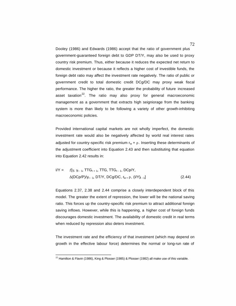
72Dooley (1986) and Edwards (1986) accept that the ratio of government plus

government-guaranteed foreign debt to GDP DT/Y, may also be used to proxy

country risk premium. Thus, either because it reduces the expected net return to

domestic investment or because it reflects a higher cost of investible funds, the

foreign debt ratio may affect the investment rate negatively. The ratio of public or

government credit to total domestic credit DCg/DC may proxy weak fiscal

performance. The higher the ratio, the greater the probability of future increased

asset taxation22. The ratio may also proxy for general macroeconomic

management as a government that extracts high seigniorage from the banking

system is more than likely to be following a variety of other growth-inhibiting

macroeconomic policies.

Provided international capital markets are not wholly imperfect, the domestic

investment rate would also be negatively affected by world real interest rates

adjusted for country-specific risk premium rw + ρ. Inserting these determinants of

the adjustment coefficient into Equation 2.43 and then substituting that equation

into Equation 2.42 results in:

I/Y = ƒ[γ, γt - 1, TTGt + 1, TTG, TTGt - 1, DCp/Y,

∆(DCp/P)/yt - 1, DT/Y, DCg/DC, rw + ρ, (I/Y)t - 1] (2.44)

Equations 2.37, 2.38 and 2.44 comprise a closely interdependent block of this

model. The greater the extent of repression, the lower will be the national saving

ratio. This forces up the country-specific risk premium to attract additional foreign

saving inflows. However, while this is happening, a higher cost of foreign funds

discourages domestic investment. The availability of domestic credit in real terms

when reduced by repression also deters investment.

The investment rate and the efficiency of that investment (which may depend on

growth in the effective labour force) determines the normal or long-run rate of

22 Hamilton & Flavin (1986), King & Plosser (1985) & Plosser (1982) all make use of this variable.

73economic growth γn. Assuming capital durability is constant, efficiency would

be monotonically associated with the output/capital ratio and thus there would be

no returns to scale, the economy would have surplus labour and the

output/capital ratio σ itself would be determined in part by the real deposit rate of

interest, as suggested in Subsections 2.2.3 and 2.3.3:

σ = ƒ(d - πe) (2.45)

A modified production function delivers the normal or long-run growth rate

function γn specified here. The investment rate I/Y is therefore the first

explanatory variable and included as a proxy for the capital stock growth rate.

The second variable affecting the rate of economic growth is taken as the labour

force growth rate lg. Finding employment data unavailable for most developing

countries, Fry assumed that unemployment remains constant.

Feder (1982) claimed that there were essentially two ways, higher marginal

productivities and externalities, through which rapid export growth could effect

economic growth rates in excess of the net export growth to GDP contribution.

By specifying this constant-elasticity externality effect, the growth rate in gross

real exports xg, is able to capture the effect solely. When scaled by the lagged

export/GDP ratio it picks up both the differential marginal productivity as well as

the externality effect. Fry (1988) does concede however, that in all his estimates

of the growth rate function, its coefficient is insignificant.

The growth rate may also be negatively affected by the variance of money

growth shocks VM, as measured by the variance of innovations to the time-series

process of money growth. Innovations are residuals of country-specific

regressions of the money growth rate on its own lagged value and a constant.

Glezakos (1978) and Leijonhufvud (1981) show that greater uncertainty with

respect to the future price level reduces output growth, while in their pooled time-

series analysis of 55 developed and developing countries, Fry & Lilien (1986)

found VM to negatively effect economic growth.

74

The function for normal (or noncyclical) growth γn was taken to be:

γn = ƒ(I/Y, lg, xg, VM)σ (2.46)

Following the Kapurian and Mathiesonian models (but in sharp contrast with the

neo-structuralist perspective) inflation was explicitly determined as the difference

between growth rates in nominal money supply and real money demand, both

measured in per capita terms. This was based on the view that inflation can be

explained proximately by the change in nominal money supply and the

determinants of the rate of change in real money demand, provided that the

money market clears within the time period under consideration. The money

market equilibrium condition being expressed:

Ms = Md (2.47)

or

Ms = P.n.md (2.48)

where Ms is nominal money supply (broadly defined to include saving/time

deposits as well as currency in circulation and demand deposits - M2), Md is

nominal money demand, P is the price level, n is population and md is per capita

demand for real money balances (Md/P)/n. It was thought reasonable, because of

the existence of auction markets, to expect market clearing conditions to hold for

annual models applied to most developing countries.

Equation 2.48 when expressed in first difference logarithmic form becomes:

∆log(Ms) = ∆log(P) + ∆log(n) + ∆log(md) (2.49)

which, when rearranged yields:

π = ∆log(Ms/n) - ∆log(md) (2.50)

where π is the continuously compounded rate of change in the price level ∆log(P)

rather than the Kapurian ∆P/P used in Equation 2.7.

75Table 2.4: Fry's Steady State Development Model

Sn/Y = ƒ[g, DR, Sf/Y, d- πe, rw, re, DCGR, DT/Y, DR.g, (Sf/Y).g, (d - πe).g, rw.g, re.g, DCGR.g,

(DT/Y).g, Sn/Yt-1] Sf/Y = ƒ[γ, rw + ρ, y/n, (DT/Y)t - 1, ε]

I/Y = ƒ[γ, γt - 1, TTGt + 1, TTG, TTGt - 1, DCp/Y, ∆(DCp/P)/yt - 1, DT/Y, DCg/DC, rw + ρ, (I/Y)t - 1]

∆(I/Y) = λ[(I/Y)* - (I/Y)t - 1] γn = ƒ(I/Y, lg, xg, VM)σ

π = ∆log(Ms/n) - θbγe - θa∆(d - πe) - (1 - θ)∆log(mt - 1) γe = E(γ) πe = E(π)

y ≡ eγ.yt – 1 P ≡ eπ.Pt - 1

γ ≡ γn + γc G = γ + TTG Y ≡ y.P I/Y ≡ Sn/Y + Sf/Y

Endogenous Variables Exogenous Variables y – Real output or GDP at constant prices

lg - Rate of change in labour force

Y – Nominal GDP xg - Rate of change in volume of exports

γn - Normal (noncyclical) real output growth rate

TTG - Rate of change in g attributable to terms of trade change

γ - Rate of change in y DR - Population dependency ratio γe - Rate of change in per capita permanent income

DT - Government and goverment-guaranteed foreign debt

I - Investment in fixed and working capital

d - Nominal deposit interest rate

σ - Output/capital ratio rw - World real interest rate Sn - National saving n – Population Sf - Foreign saving (balance-of-payments deficit on current account)

ε - Exchange rate overvaluation

ρ - Country specific risk premium r - Real return on investment g - Growth in real income re - Expected real return on investment π - Inflation rate DCp - Domestic credit to the private

sector πe - Expected inflation M - Money stock (broadly defined to

include all bank deposits) mt - 1 - Lagged real capita money stock

Source: Fry (1988)

Only through an analysis of the determinants of both nominal money supply and

real money demand can the inflationary process be fully determined. Aghevli &

Khan (1977) show, however, that provided any feedback from inflation to money

supply growth occurs with a lag, the model is recursive. Then, for the purpose of

76estimating inflation, changes in the nominal money supply can be treated as

exogenous. Real money demand is normally specified as a function of one or

more price (interest rate) variables and a budget constraint. In this model the

price variable was taken as the real deposit rate of interest d - πe, and the budget

constraint was the per capita permanent or expected real income yp. The long-

run or desired money function then took the form:

m* = cybpe

a(d - π↑e) (2.51)

where m* is the desired or long-run level of real money balances and a, b, and c

are constants.

Adjusting the actual level of real money balances with a lag to changes in the

determinants of money demand, requires that short-run or actual money demand

be specified:

log(md) = log(mt - 1) + θ[log(m*) - log(mt - 1)] (2.52)

Some fraction θ of the gap between desired and actual money balances held in

the previous time period is eliminated in the current one. Combining Equations

2.51 and 2.52 and expressing it in first difference logarithmic form creates:

∆log(md) = θb∆log(yp) + θa∆(d - πe) + (1 - θ)∆log(mt - 1) (2.53)

Taking γe as the rate of change in per capita permanent income ∆log(yp) and

substituting Equation 2.53 into Equation 2.50, yields:

π = ∆log(Ms/n) - θbγe - θa∆(d - πe) - (1 - θ)∆log(mt - 1) (2.54)

The implications of this model are also glaringly obvious. In the steady state,

increasing the nominal deposit rate would raise the real deposit rate toward its

equilibrium free-market level. This may then increase the savings rate, raise the

average efficiency of the greater volume of investment that can now be

77undertaken, reduce the rate of inflation and thus would raise the real deposit

rate even further.

2.4 Extensions to the McKinnon and Shaw Models

While both McKinnon and Shaw did discuss dynamic aspects of repression and

liberalisation, neither constructed a formal dynamic model. McKinnon (1973)

pointed out that stabilization programmes implemented by monetary contraction

invariably produced an initial rise in circulation velocity (using the broad M2

definition of money) and thereby a credit squeeze in real terms. Declining

inflation would only later raise real money demand and thus reduce velocity.

Blinder (1987) has confirmed, from both demand and supply sides, that there is

little dispute a credit squeeze is contractionary.

Section 2.3 has shown that the models developed by Kapur (1976a), Mathieson

(1980) and Fry (1988) incorporate dynamic adjustment mechanisms, while

Galbis's (1977) did not. In the Kapurian model McKinnon's observation about

initial velocity-rises through money market disequilibrium is caputured. Both

Kapur and Mathieson use adaptive expectations in their earlier models and

rational expectations in their later papers, while Fry had always taken

expectations based solely on past values of the variables themselves. Kapur

employed a Phelpsian expectations-augmented Phillips curve, while Fry used a

Fisherian expectations-augmented Phillips curve. Shaw (1973 : 234) himself

noted that "Delayed responses to stimuli are essential elements of the models,

and these may be attributed to technology, behavioural preferences, and

imperfect foresight". Section 2.4.1 below, compares the dynamic properties of the

three financial development models.

Rational expectations have now replaced adaptive expectations in mainstream

macroeconomic literature. Expectations are formed rationally when people make

efficient use of information on past inflation and other variables that are available,

in order to avoid systematic mistakes (Barro, 1987). The incorporation of rational

expectations in deterministic models is equivalent to perfect foresight. In that

78case, using adaptive expectations would be a convenient way of allowing

expected inflation to differ from actual inflation, at least in the short run. The

contractionary effects of monetary deceleration would follow, provided part of any

reduction in the inflation rate was unexpected. The stochastic versions of all the

dynamic models reviewed in this Section can easily accommodate rational

expectations for purposes of estimation.

Korea, as part of its financial and fiscal reforms of 1964-1965, devalued its

currency from 130 Won to 270 Won to the Dollar, that exchange rate being

supported (in part) by liberal government exchange rate guarantees. As there

was general confidence in the new rate's sustainability, the high nominal interest

rate provided a strong incentive for short-term capital inflows. Monetary control

was however jeopardized by the resulting increase in net foreign assets. In light

of the Korean experience both McKinnon and Shaw had much to say about

balance-of-payments and exchange rate policies. Although, neither provided any

formal framework for their analyses. McKinnon (1973) and Shaw (1973) both saw

flexible exchange rates policies as crucial elements in their optimal financial

stabilization and liberalisation programmes. Nominal interest rates, they argued,

had to be set at relatively high levels at the outset of transitions, because

inflation, or at least expected inflation, does not decline immediately after reform.

McKinnon (1973 : 166-167) advocated the adoption of a crawling peg, which

would deter undesired and disruptive capital inflows, thereby maintaining both

interest rate and purchasing power parity during deflation. Shaw (1973 :221-226),

on the other hand, preferred a floating exchange rate together with its

requirement of full convertibility. Still, in a less than perfect world, he was willing

to support a crawling peg (Shaw, 1976).

Section 2.4.2 discusses some of these open economy extensions to the M-S

approach. Kapur (1976) and Mathieson (1980) both introduced foreign trade and

the exchange rate into their formal models, the exchange rate being an additional

policy instrument. Still the optimal exchange rate policy during stabilization

derived from the Kapurian model differed substantially from Mathieson's. Fry's

79(1988) open economy extension added a foreign trade sector to the model

presented in Subsection 2.3.4 and endogenized both the real exchange rate and

the terms of trade.

2.4.1 Dynamic Extensions

Kapur (1976a) postulated two sources of dynamic adjustment - money market

disequilibrium and adaptive expectations of the inflation rate. Adaptive

expectations being expressed:

dπe/dt = β(π - πe) (2.55)

where πe was the expected inflation and π the actual inflation rate. Money market

disequilibrium was included in an expectations-augmented Phillips curve:

π = h [(Ms/PY) - (Md/PY)] + πe (2.56)

where Ms stood for the money supply, Md for money demand, P the price level

and Y real GDP. Excess supply of money equals excess demand for goods in a

two-market economy. Thus Equation 2.56 is a transformation of the standard

expectations-augmented Phillips curve, with excess demand being proxied by

the gap between actual and trend output, which is itself used in place of excess

money supply. Equation 2.56 shows that markets do not clear instantaneously,

but that rather excess demand for goods causes producers to raise prices faster

than the expected inflation rate until the excess demand is eventually eliminated.

Equation 2.56 could also incorporate a stock adjustment mechanism for the gap

between desired and actual real money balance holdings. Laidler (1978) has

identified Equation 2.56 as being a Phelpsian version of the expectations-

augmented Phillips curve. By defining W as the logarithm of velocity of circulation

V, the Kapurian model can be reduced to two equations of motion:

∆W = - µ[ 1- (σq/1 -α) e-W] + (1 - θ)πe+ (1 - θ)[e-W - ea(d - π↑e)] (2.57)

dπe/dt = βh [e-W - ea(d - π↑e)] (2.58)

80Two alternative stabilization policies may then be introduced to stimulate an

economy experiencing excessive inflation and thus, low growth. Analytical

solution being intractable, stimulation becomes necessary. The first policy is to

reduce the rate of monetary growth µ, which would produce a phase of rising

velocity W, inflation πe would be expected to fall, followed by a phase of falling W

and falling πe, followed hopefully by cyclical convergence to a new equilibrium23.

Monetary deceleration would produce the initial velocity acceleration stressed by

McKinnon.

Expressing the Kapurian growth equation in terms of the logarithm of velocity W

gives:

γ = µ[σq/(1 - α)] e-W - πθ (2.59)

The rate of economic growth γ, is reduced by both the initial fall in the money

growth rate as well as the rising velocity, W, of the first phase. Equation 2.58

shows that this rising velocity would produce a declining inflation rate. Reducing

the monetary growth rate µ, cuts the net flow of real bank credit, immediately

reducing the rate of economic growth γ. The negative effects of rising velocity on

the rate of economic growth are then, partly, fully or more than offset by falling

actual and expected inflation. When W and π both fall, γ will be above its long-run

equilibrium level to which it will then converge.

Raising the deposit rate of interest toward its equilibrium level constitutes the

second policy. Here, the logarithm of velocity W as well as expected inflation πe

would both fall in the initial phase. The increase in d would raise real money

demand immediately thereby initially lowering the inflation rate π, since there is

no jump in W or πe. Equation 2.59 shows that an initial cut in π raises γ. The

falling W and π of the first phase, raise γ causing it to overshoot its new higher

23 Falling W, raising πe, rising W, rising πe, rising W, falling πe, falling W, falling πe (Kapur, 1976a : 787).

81equilibrium value, to which it then converges. An upward shift in d has

favourable effects of γ and π in both the short-run and the steady state (Kapur,

1976 : 792).

The optimal policy with regard to d would thus be to set it (or better still allow it to

rise through competitive forces) to its upper bound, which would equal r* + πe

when the cost of bank intermediation and reserve requirements are assumed to

be zero (q equal to 1). When q = 1, d = r* + πe and θ < 1, the growth maximizing

value of µ is ∞, as shown in Subsection 2.3.1. Despite this the Kapurian model

clearly illustrates the dynamics of two alternative stabilization policies, showing

vividly the superiority of financial liberalisation through the abolition of interest

rate ceilings, over monetary contraction alone as a stabilization device.

In later papers Kapur (1982; 1983) applied control theory techniques to solve the

optimal stabilization problem. He included target values for π and W in the

government's loss function and in most cases set the nominal deposit rate, d, at

its upper bound throughout the transition. While he did concede that the deposit

rate may have to be set below its upper bound, to deter excessive capital inflows

in his open economy model, at least during the transition period (Kapur, 1983), in

all cases the optimal solution was found by setting d at its upper bound in the

steady state.

Optimal transition paths invariably require initial discrete changes in µ and d,

which are then followed by smooth convergence to steady state values.

However, optimal transitions may require changes from minimum to maximum,

intermediate to minimum or maximum, minimum to maximum or intermediate and

maximum to minimum values of µ and d. These changes may occur in some

instances of cyclical convergence and in fact switches in policy instruments from

one extreme to another are quite typical of dynamic control model solutions.

However, they clearly highlight the practical and political difficulties of this

technique for economic policy making.

82Mathieson (1980) also incorporates two sources of dynamic adjustment to his

model, a decaying stock of fixed-interest bank loans as well as adaptive

expectations of the inflation rate. He assumes rates on bank loans are fixed for

the duration of the loan and it therefore takes time for banks to replace low

interest loans with higher interest ones after liberalisation. Indeed, Mathieson did

warn that liberalisation could disrupt established financial institutions holding a

portfolio of low yielding pre-reform loans. New entrants that had earnings from

portfolios consisting solely of higher yielding post-reform loans could attract

deposits away from the existing institutions. Competing with these new entrants

could completely erode the net worth of the existing institutions. He specified the

government's loss function in terms of target inflation πt and growth rates γt:

U = δ1(π - πt) + δ2(γ - γt)2 (2.60)

where δ1 and δ2 are both positive. Subject to the constraints that money and

credit markets remain in continuous equilibria and that no bankruptcies of

established financial institutions occur, this loss function may be minimized by

employing the policy instruments µ, d, and l (the nominal loan interest rate).

Equations 2.19 and 2.20 show that money and credit market equilibria can be

maintained if and only if ∆d = ∆πe, which requires the real deposit interest rate be

held constant. The real loan rate is first set above its steady state level and

reduced gradually as pre-reform loans are repaid, with the average real loan rate

remaining constant at the zero profit level for existing institutions.

New entrants will be attracted by the wider gap between transition deposit and

loan rates but they will be prevented from engaging in price competition. At all

times after the reform is initiated the real deposit rate d - πe is held at its

equilibrium level (shown as r2 in Figure 2.4).

Assuming the economy starts off financial repressed with high inflation and low

growth, the optimal strategy would be an initial discrete increase in both d and l,

provided that the loan rate was held below its market clearing level. Then a

83discrete decrease in µ to a rate below its long run value would be needed.

During the transition d and l should be gradually reduced, d in step with πe,

although l somewhat faster, µ must also be raised, gradually, to its steady state

value congruent with π = πt. The growth rate would initially experience a discrete

increase and then rise toward γt. Inflation would simultaneously decline toward πt,

the model not permitting any cyclical convergence.

The low fixed-interest bank portfolio feature needlessly complicates Mathieson's

(1980) model. As Section 2.3 has described, the effective loan rate, under

conditions of repression is likely to be above rather than below its competitive

level and, anyway, government-set bank loan rates in a number of repressed

economies are automatically adjusted whenever the official rate structure is

changed. In Korea and Taiwan for example, following upward revisions of the

institutional interest rate structure, simple alternative techniques to prevent

bankruptcies have been used.

In the Mathiesonian model the growth rate target is attained so soon as the real

loan rate l - πe is set at its steady state value. Provided that bank loan rates are

variable or adjustable and that a competitive nominal return is paid on bank

reserves (making q = 1) this can be done at the very start of a stabilization

programme. Without interest being paid on reserves, the real loan rate will fall

and the growth rate together with inflation will rise. It is only when there is no

required reserve ratio or when these reserves earn a competitive rate that the

adaptive mechanism affects the path of actual inflation. This is as money is

neutral even during transition. However, with rational expectations and a pre-

announced credible stabilization programme, provided there are no low fixed-

interest rate loans in bank portfolios, µ, d, and l, can all be set at their steady

state values at the very beginning.

Essentially the differences between the Kapurian and Mathiesonian models lie in

the growth rate functions as well as Kapur's market disequilibrium mechanism.

This gives Kapur the possibility of cyclical convergence and thus of discrete

84switches in policy instrument values. In the Mathiesonian model, since cyclical

convergence never occurs, after initial discrete changes, policy instruments are

always monotonically changed during the transition period. Considerations that

are not incorporated in either of the models, determine the setting of an

independent inflation target. In the Mathiesonian model growth maximization

requires an inflation rate of -∞, provided q < 1. While Figure 2.8 shows that in the

Kapurian framework a finite inflation rate for growth maximization is produced.

With q = 1 or a competitive return on required reserves, money is neutral in the

Mathiesonian framework. In the Kapurian context growth is maximized when

inflation is infinite.

Fry's (1988) model includes the same sources of dynamic adjustment used in the

Kapurian model, adaptive expectations of the inflation rate, the price level, and

the growth rate in per capita real permanent income. Together with an

expectations-augmented Phillips curve as well as the various adjustment lags

specified in Subsection 2.3.4. However, his adaptive mechanisms are a bit more

general than that used by the other two authors:

πe = m∑i=0 αiπt - i (2.61)

γe = n∑j=0 βjγpc

t-j (2.62)

where γpc is actual per capita income growth and γe is permanent per capita

income growth. The lag coefficients αi and βj are constrained to sum to 1 and

either decline monotonically or form an inverted U pattern. A dynamic adjustment

mechanism for the inflation Equation 2.54, which already has a stock adjustment

lag for real money balances, is given by the response lags specified in Equations

2.61 and 2.62. Rewriting Equation 2.54 in terms of Kapurian and Mathiesonian

symbols yields:

π = µ - ν - bγe - a∆(d - πe) - c(µ - π - ν)t - 1 (2.63)

where ν is the population growth rate.

85The money market's equilibrium condition, of demand equalling supply, is

used to derive Equation 2.63. On the other hand, whenever there is repression,

the credit market remains in disequilibrium. From Walras's Law disequilibrium in

one market must be matched by an equal and opposite disequilibrium in one or

more other markets and it is natural to think of an excess demand for credit being

matched by an excess supply of money. However, seeing credit market

disequilibrium as an excess supply of bonds at an administratively fixed interest

rate, requires that it be matched by planned investment exceeding planned

saving at that particular interest rate. In which case, planned investment does not

represent effective investment demand since it is contingent upon obtaining

investible funds at the fixed interest rate. Effective investment demand is

constrained by a lack of credit to equal saving that occurs at the fixed interest

rate. Price changes can equilibrate demand for and supply of money, allowing

money market equilibrium to coexist with credit market disequilibrium.

Lucas (1973) suggests that, because of the preponderance of auction markets or

faster expectation responses in developing economies, prices may adjust in

disequilibrium more rapidly here than in industrialized countries. Thus, as pointed

out in Subsection 2.3.5, for models estimated using annual observations, it may

be reasonable to expect money market equilibrium to hold. Further, following the

introduction of monetary deceleration, circulatory velocity tends to fall back after

a rise, within 12 months. This means that money market disequilibrium, though

important, tends to be eliminated by price adjustment within an annual period.

Fry's (1988) money market equilibrium contrasts with Kapur's dynamic

mechanism that relies in part on money market disequilibrium. On the other

hand, the Mathiesonian framework specifies its optimal stabilization strategy as

one that establishes immediately and then maintains money and credit market

equilibrium.

Laidler (1978) posits that being consistent with the argument used to justify

money market equilibrium requires that a Fisherian Phillips curve be used in

preference to a Phelpsian Phillips one. The Fisherian Phillips curve determines

86the actual rate of economic growth γ. It is determined by the ratio of the actual

to expected price level P/Pe or, alternatively the difference between actual and

expected inflation π - πe. The expected price level, Pe , is eπ↑e.Pt - 1. If actual price

or inflation exceeds what was expected, entrepreneurs read the difference as a

real increase in demand for their products. Thus they raise the capacity utilization

rate of existing capital in order to increase short run output and invest more to

increase that capacity in the longer run. The higher the difference, the better the

investment outlook appears and the greater the rate of economic growth

becomes. That's why P/Pe or π - πe can proxy re in the saving function Equation

2.37.

Short run growth is also affected by expected inflation through real deposit

interest rates d - πe. In repressed developing economies under the disequilibrium

interest rate and foreign exchange control systems that exist, real money

demand determines to a great extent real supply of domestic credit. Which, in

turn, is the primary asset backing the monetary liabilities of the banking system.

With accelerating inflation and falling real deposit interest rates, the government

expropriates an increasing proportion of the declining supply of real domestic

credit to fund its current expenditures24. Thus funds for both fixed and working

capital are doubly squeezed.

Traditionally the link between credit and output is through demand, monetary

expansion creates an increase in credit accompanied by an increase in demand

which stimulates real output. However, since 1973 a number of economists have

focused on the link between credit and demand through the supply side25.

Essentially a Wicksellian view it holds that the availability of working capital

determines, ceteris paribus , the volume of production that can be funded. As

24 Aghevli & Khan (1977; 1978), Dutton (1971), Ness (1972), and Uluatam (1973) all discuss this phenomenon. 25 The pioneering works on this perspective are from Blinder (1987), Buffie (1984), Cavallo (1977), Fry (1980b), Kapur (1976a; 1976b), Keller (1980), Mathieson (1980), Taylor (1983), van Wijnbergen (1982; 1983a; 1983b).

87Keller (1980 : 455) puts it: "production expansion may depend, entirely or in

part, on credit availability and/or the cost of credit". This supply link between

credit availability and real economic growth comes from either the ratio of credit

to output or from its real as opposed to nominal volume.

The inflation rate rises during periods of faster monetary and nominal credit

expansion. Under conditions where the nominal deposit rate is fixed, the ensuing

increases in expected inflation would reduce the real deposit interest rate and in

turn reduce real money demand, or decrease the ratio of money to nominal

output. Even if domestic credit expansion were the cause of monetary

acceleration the ratio of domestic credit to nominal output may still fall. This

would happen if domestic credit expansion reduced net foreign assets by less

than the amount of the expansion. Hence, acceleration in nominal domestic

credit and thereby in money supply would reduce the availability of credit in real

terms.

The government may find that the gap between conventional tax receipts and

public expenditure widens, as inflation accelerates and real deposit rates, real

money demand and real credit supply all fall. This bigger gap must then be

financed either by heavier reliance on seigniorage or the inflation tax. The

government could extract greater seigniorage by increasing that proportion of

domestic credit allocated to the public sector, effectively reducing the ratio of

private sector credit to total domestic credit. Or it may levy an inflation tax by

issuing more money than the public wishes to hold at current prices, producing a

double squeeze on credit available for private sector working capital. In Turkey

for instance, the velocity of circulation (measured by M2) rose by 70 percent and

the ratio of public sector domestic credit to money supply increased from 20 to

229 percent as the expected real deposit interest rate fell from 0.2 percent in

1970 to -22.7 percent in 1980. As the real supply of domestic credit declined and

the government extracted a higher seigniorage from money supply, the private

sector was starved of credit. Finance for working capital dried up and the credit

squeeze reduced the capacity utilization rate of the existing fixed capital stock

(Fry, 1979a). The growth rate declined. In reduced-form equation, d - πe, thus has

88a positive effect on γ, by determining credit availability as well as the allocative

efficiency of loanable funds.

As introduced in Subsection 2.3.4, the normal growth rate γn also affects actual

growth. In fact the difference between γ and γn, defined as z, is determined by

P/Pe and d - πe:

z = ƒ(P/Pe, d - πe) (2.64)

Normal (noncyclical) growth is affected by variations in weather conditions which

determine in part fluctuations in agricultural output. Hemphill (1974) and Krueger

(1974) both identify fluctuations in import levels26, as being exogenous or

noncyclical phenomena in repressed economies that maintain disequilibrium

foreign trade regimes subject to tight government control. Normal growth when

defined to include fluctuations around the long-run trend in agricultural output, γna,

has a positive effect on γ. Above-average growth in agricultural output however,

depresses growth in other sectors of the economy due to another credit effect.

Credit demands of other sectors are effectively crowded out by the credit

requirements of agricultural price support programmes that are positively related

to growth in agricultural output. Thus, when more of the fixed real supply of

domestic credit is allocated to agriculture, other sectors suffer a credit squeeze in

real terms. This implies that while the effect of γna on γ is positive, its coefficient is

less than one, despite that, on average γ equals γna. The credit squeeze on the

other sectors of the economy, caused through above-average agricultural

growth, reduces those sector's capacity utilization rates and thus produces

below-average growth there. Th us:

γ = ƒ(γna, P/Pe, d - πe) (2.65)

26 Mainly of raw materials, semi-f inished goods and capital equipment that act as factor constraints to output in the short-run.

89At this stage it may be useful to compare the short and long-run inflation and

growth tradeoffs implied by the three models under review. The comparison is

made with d being artificially held below its competitive equilibrium level. The

policy implications of all three models are the same, that an increase in d toward

its equilibrium level, both raises γ and reduces π simultaneously. Figure 2.8

shows these short and long run Phillips curves under repressed conditions.

Fig. 2.8: Short & Long Run Phillips Curves

in the Three Financial Development Models

Source: Fry (1988)

2.4.2 Open Economy Extensions

Kapur (1983) and Mathieson (1979a) both developed open economy models of

repressed countries, where the exchange rate became an additional policy

instrument. By allowing the exchange rate to deviate from purchasing power

parity, their extensions brought considerable complexity to their earlier models.

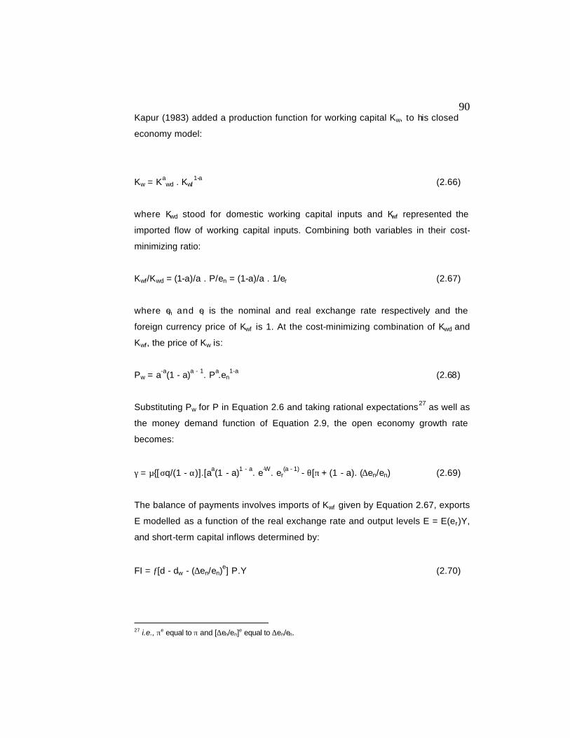
90Kapur (1983) added a production function for working capital Kw, to his closed

economy model:

Kw = Kawd . Kwf

1-a (2.66)

where Kwd stood for domestic working capital inputs and Kwf represented the

imported flow of working capital inputs. Combining both variables in their cost-

minimizing ratio:

Kwf/Kwd = (1-a)/a . P/en = (1-a)/a . 1/er (2.67)

where en and er is the nominal and real exchange rate respectively and the

foreign currency price of Kwf is 1. At the cost-minimizing combination of Kwd and

Kwf, the price of Kw is:

Pw = a-a(1 - a)a - 1. Pa.en1-a (2.68)

Substituting Pw for P in Equation 2.6 and taking rational expectations27 as well as

the money demand function of Equation 2.9, the open economy growth rate

becomes:

γ = µ{[σq/(1 - α)].[aa(1 - a)1 - a. e-W. er(a - 1) - θ[π + (1 - a). (∆en/en) (2.69)

The balance of payments involves imports of Kwf given by Equation 2.67, exports

E modelled as a function of the real exchange rate and output levels E = E(er)Y,

and short-term capital inflows determined by:

FI = ƒ[d - dw - (∆en/en)e] P.Y (2.70)

27 i.e., πe equal to π and [∆en/en]e equal to ∆en/en.

91where dw represents the world nominal interest rate. The complete balance of

payments equality could now be written:

∆R = P.E - enKwf + FI (2.71)

where ∆R is the nominal change in net foreign assets.

Domestic cash C, net foreign assets R and loans L support money. C remains a

transfer payment, controlled to manage monetary expansion: L/M = q, (C + R)/M

= 1 - q, and (∆C + ∆R)/(C + R) = ∆M/M = µ. This monetary control assumption is

clearly at odds with reality in many developing countries. Fry (1988) therefore

employed an alternative money supply process in his model, although admittedly,

the problem of monetary control in practice is still a critically unresolved issue in

this field.

Kapur's (1983) open economy model thus has three target variables - er, W and

π - together with three policy instruments for achieving them - d, µ and υ [where υ

is ∆log(er)]. The government has three objectives, to create a nonnegative trade

balance, to lower inflation and to raise economic growth rates. The economy is

assumed to start from a situation of trade deficit, high inflation and low growth.

The transition process to minimize the loss function G:

G = �0∞ e-ρt [m1(W -Wt)2 + m2(π - πt)2] dt (2.72)

where ρ, the discount rate, involves discrete and continuous changes in d, µ and

υ.

The main policy implication from this model is that the real exchange rate

(nominal rate adjusted for relative inflation at home and abroad) may have to be

depreciated during the transition from repression to liberalisation. Although, it

may not necessarily be optimal to value the rate, at first, by the full extent

required for steady state trade balance. Such a devaluation could produce

excessive short-term capital inflows, a problem Korea faced in the 1960s and

Chile in the 1970s. On the one hand, Equation 2.69 shows that a high real rate of

92depreciation υ during transition will reduce γ. On the other, a high value for υ

allows a high value for d, as the real exchange rate would start well below its

target value and the rate of return on working capital r*, is inversely related to re:

r* = [P.Y - PwKw]/PwKw

= [σ/(1 - α)].[aa(1 - a)1 - a. era - 1 - 1] (2.73)

Under certain initial conditions, the optimal value of υ lies somewhere between

an arbitrarily imposed lower bound of zero and an upper bound where capital

flight is induced. In that case, a positive value for υ supports strong deflationary

measures at some cost to growth foregone.

Mathieson (1979a) also extended his earlier closed model for the open economy

and at the same time did away with the assumption of a low fixed-interest loan

portfolio that encumbered it. In addition to balance-of-payments considerations

his later model contained a Phillips curve:

π = φlog(Q/Y) (2.74)

where Q is aggregate demand and Y aggregate supply in real terms. The rational

expectations he adopts28 is the sole source of dynamic adjustment in his model.

Here π refers to the rate of change in the price of domestic goods. Aggregate

demand for domestic output is a function of domestic income Y, foreign income

Yf , expected inflation πe and the relative price of domestic (P) to foreign goods

(Pf ) converted through the exchange rate en into domestic currency units:

log(Q) = r0 - r1log(P/enPf ) + r2log(Y) + r3πe + r4log(Y f ) (2.75)

where r1, r2, r3 and r4 are all positive.

The general price level in this model is then defined as:

Pg = Pε(enPf )1 - ε (2.76)

28 πe = π and xe = x, where x is the rate of change in the nominal exchange rate.

93where ε is the weight attached to the domestic goods price.

Equation 2.16 still gives loan demand and the rate of capital accumulation is also

unchanged from Equation 2.17. Equation 2.20, which gave the deposit demand,

changes as a substitute financial asset in the form of foreign deposits with a yield

dw is introduced:

D/Pg = ƒ(d - πge, dw + xe - πg

e)Y (2.77)

All money is held as deposits and the ratio of deposits to high-powered money H

is fixed: D = (1 - q)H. Similarly to Kapur's open economy model, high powered

money equals C + R. In fact, Mathieson (1979a) confusingly defines H to equal

domestic credit DC plus reserves, although DC is not credit since it is not added

to L. It seems that Mathieson created DC as a transfer payment in much the

same way that Kapur created C. In contrast with The Kapurian alternative,

however, government here can control µ or x but not both. If x is the chosen

policy instrument then D is demand determined and C affects the overall balance

of payments position only.

If purchasing power parity were imposed then the Mathiesonian model would

collapse, making it interesting that µ and x cannot be used as independent policy

instruments. The technical explanation being that the disequilibrium in

Mathieson's money market does not affect the price level directly (Equations 2.74

and 2.75). The only equilibrating mechanism being a change in en, which affects

Q, which has a knock-on effect on π. Thus, if en is the policy instrument chosen,

money market equilibrium can only be achieved through corresponding changes

in H.

Mathieson's (1979a) open economy model has no equilibrating mechanism.

Moreover balance-of-payments equilibrium can only be achieved through C

policy (the simplest monetary approach to balance of payments), despite the

substitutability between domestic and foreign goods and financial assets being

less than perfect. This is because of a requirement that C + R must equal the

94demand determined D/(1 - q). The absence of any behavioural determinants

of the balance-of-payments position is also a disturbing lacuna.

The lack of any equilibrating money market mechanism is perhaps the most

serious flaw in the Mathiesonian framework. By simply allowing money market

disequilibrium to spill over directly into the domestic goods market, which seems

quite reasonable for any developing economy, independent monetary and

exchange rate policies could be permitted. Rather, because the model assumes

the monetary authority adjusts the deposit rate to prevent disequilibrium at all

times no spillover effects can occur. Under these circumstances it is unnecessary

to model any equilibrating mechanism. Why a model, in which interest rates are

constrained to take their market clearing values, would be built to analyze the

transition from repression to liberalisation therefore seems anomalous. To be fair

the model itself does not purport to describe the financially repressed economy

but rather a developing economy under the benign influence of equilibrating

financial policies.

Under rational expectations, imposing equilibrium in money and credit markets

as a requirement for an optimal stabilization program requires:

µ - επ - (1 - ε)x = γ (2.78)

since D/Pg equals θ(K/q) and πg equals επ + (1 - ε)x, velocity of circulation has to

be kept constant.

Logarithmic differentiation of Equation 2.77 with respect to time yields:

µ - επ - (1 - ε)x = (f1/f) [∆d - ε∆π - (1 - ε)∆x] + (f2/f) [∆x - ε∆π - (1 - ε)∆x] + γ (2.79)

when dw is constant. The nominal deposit interest rate needs to be changed to:

∆d = ε(1 + η) ∆π + [1 - ε(1 + η)]∆x (2.80)

where η equals f2/f1, required to maintain constant velocity.

95Mathieson (1979a: 458) demonstrates a dynamic solution to his model by

assuming the economy starts from a position of "rapid inflation, low or zero

growth and a balance of payment deficit". He then uses Equation 2.74 to show

that price stability could be approached through an initial discrete increase in d

and l, an overdepreciation of en and a decline in the growth rate of C. The

instantaneous effect is an upward jump in γ as a result of the liberalisation. After

these discrete changes, the economy could approach its steady state through a

gradually appreciating exchange rate, gradual reductions in d and l as well as a

gradual increase in C at a rate lower than µ. During this transition γ may

gradually decline to its steady state value, inflation should fall and the balance of

payments return to equilibrium after capital inflows generated by appropriate

control over C have occurred during the transition.

Exchange rate policy provides the reason economic growth would be above its

steady-state value during transition. Initially overdepreciating the domestic

currency should produce expectations of subsequent appreciation in er. A decline

in the expected nominal depreciation, given levels of d and dw, would, according

to Equation 2.77, raise deposit demand. Ceteris paribus the more er is expected

to appreciate, the less en will be expected to depreciate. Thus the greater the

initial overdepreciation, the lower the value for d - πge required to generate a

given demand for deposits would be. In turn, a lower real deposit rate would

allow a lower real loan rate l - πge which would encourage faster capital

accumulation and thus a higher economic growth rate. Overdepreciation would

also deter capital flight by reducing the attractiveness of foreign financial assets.

Equations 2.74 and 2.75 also suggest that the greater the overdepreciation, the

higher the domestic inflation rate, brought on by a greater demand for domestic

goods, will be. By increasing the spread between d and l, due to the inflation tax

being levied through noninterest-bearing bank reserves, this higher inflation

would reduce growth. Thus, there is an optimal extent of overdepreciation at

which a lower value of xe on d exactly offsets the effect of a higher πe on both d

and l, such that l -πge is minimized.

96At a nominal loan rate l, (equal to r* + πe in the Kapurian framework) demand

for loans is infinitely elastic. This means that depositors alone bear the inflation

tax levied through bank reserves. In the Mathiesonian framework demand for

loans is not infinitely elastic, that's why a higher l - πge value would reduce capital

accumulation and thereby economic growth. Still, the equilibrium deposit rate is

invariant to the rate of economic growth, needing to be set at a level that

generates a deposit/income ratio equal to θ/σq29 . So the higher the required

reserve ratio 1 - q, the higher the market equilibrating value of d will be. In this

case the inflation tax is borne wholly be borrowers. Far from being growth raising,

as in the Kapurian framework, in Mathieson's model, inflation always reduces

growth, as expectations in both these models are rational.

Mathieson's (1979a) open economy model needs a number of comments. First, if

πe deserves a place in the demand for goods function (Equation 3.75) then by the

same logic do d, dw, and xe. As with πe, the signs of their coefficients are

ambiguous in theory and empirical evidence suggests that higher real deposit

rates reduce aggregate demand in several countries (c.f., Boskin, 1978; Fry,

1978c; 1979a). Including d in Equation 3.75 could produce a sharp deflationary

impact at the start of the stabilization programme, which might more than

counteract the inflationary impulse of devaluation.

Second, logic and consistency also dictate that dw and xe be included in the

investment/saving function. Rather than just investing domestically entrepreneurs

could also buy foreign bonds30. (As already stated Kapur specified neither a

saving nor an investment function). In an inside money economy in which money

itself enables decisions to save to be taken independently from decisions to

invest, separate saving and investment functions are a necessity.

29 Since L/Pg = θK, D/Pg = f.Y = f.σK, and L=qD. 30 Although the problem here is probably the lack of separate saving and investment functions, a defect stemming from McKinnon's (1973) self-finance model.

97Finally, overdepreciating a currency during transition to obtain a rate of

economic growth above equilibrium is repeatable. It is quite plausible that a

series of discrete devaluations followed by gradual appreciation would always

make foreign assets less attractive to domestic deposit holders, keeping growth

perpetually above its steady state. Of course, this happy scenario would only be

possible if depositors irrationally failed to anticipate future devaluations. They

must therefore rationally anticipate irrational government policy until a rational

stabilization programme is initiated as a complete surprise. Simply, they must not

anticipate a large devaluation. From then on, government policy is expected to

aim toward bringing the economy to a steady state.

Regarding devaluation strategy, Mathieson's (1979a) model leads to conclusions

contrary to those derived from Kapur. Mathieson has argued that an initial

overdepreciation of the real exchange rate followed by a gradual appreciation

would maintain economic growth rates above their steady state values during

transition. This as the real deposit rate required to generate any given demand

for real money balances is reduced because a real term appreciation of the

domestic currency is expected. The resulting lower real deposit rate allows a

lower real loan rate that encourages faster capital accumulation and thus higher

economic growth rates. The initial overdepreciation deters capital flight by

reducing foreign financial asset attractiveness.

The fundamental difference between the exchange rate polices advocated by the

Kapur and Mathieson schools come from several places. First, in the Kapurian

framework the real rate of return on working capital r* is negatively related to the

real exchange rate. A higher r* permits a higher d - πe, which is both deflationary

as well as growth accelerating. Second, returns from foreign financial assets,

adjusted for changes in the exchange rate, do not affect money demand. Thus in

the Kapurian framework faster depreciation during transition does not reduce real

money demand. In sharp contrast, the Mathiesonian framework has the

exchange rate adjusted returns from foreign assets affect money demand.

Investment and growth from this perspective is raised by the lower real loan rate

98together with the lower deposit rate, an appreciation of the real exchange rate

during transition, makes possible.

Fry's (1987) open economy extension simply brings in export and import

functions and endogenizes both the exchange rate as well as terms of trade. As

an open developing country faces an infinitely elastic supply of imports, its import

volume is determined solely by its own demand. The prices of exports, imports

and nontradable goods affect this demand. Its income elasticity may be unitary

but the composition of GDP affects imports. Particularly, investment is more

import -intensive than consumption and thus the ratio of imports to GDP is

determined, in part, by the ratio of investment to GDP I/Y. Finally, adjustment to

the desired import level may be limited by the availability of foreign exchange that

exporters earn. In many developing countries quantitative restrictions on imports

of consumer goods are imposed. Typically, licenses to import them are rationed

out not on the basis of foreign exchange availability but rather on the availability

of nonborrowed foreign exchange or foreign exchange earned by exporters. The

import demand equation IM/Y, when expressed as a ratio of imports to GDP

(both at constant prices) takes the form:

IM/Y = ƒ(REX, TTI, I/Y, XP/PY, IM/Yt - 1) (2.81)

where the real exchange rate REX is used to proxy the relative price of

nontraded goods to imports, TTI is a ratio of export to import prices (or the gross

barter terms of trade) and XP/PY is the ratio of nominal exports to GDP.

Schadler (1986) and Sundararajan (1986b) agree that the volume of exports is

both demand and supply driven. Export supply is determined by the prices of

exports and nontraded goods, with its supply function Xs/Y expressed as the ratio

of exports to GDP (again both at constant prices):

Xs/Y = ƒ(REX, X/Yt - 1) (2.82)

99Demand for developing country exports is determined both by export and

import prices as well as by income growth in the member countries of the

Organization for Economic Co-operation and Development (OECD). The export

demand function is thus written:

Xd/Y = ƒ(TTI, γw, X/Yt - 1) (2.83)

where γw is income growth in OECD countries.

These three additional equations are used to determine the real exchange rate,

the terms of trade and the volume of exports or imports. The volume of imports

can be derived from the current account balance given by the difference between

national saving and domestic investment, assuming that exports are determined

by this block. In other words, IM = X - CA, where CA is the current account

surplus and CA = Sn -I or IM = X + Sf and Sf = I - Sn. Given this foreign trade

block, Fry's (1987) model could be used to simulate export promotion and import

compression policies. Such simulations would show the changes in real

exchange rates as well as the terms of trade produced by these policies and their

growth rate implications.

2.5 Effects on Saving, Investment and Growth

Financial restriction quickly turned to repression over the worldwide inflation of

the 1970s, or worsened the lot of those industrial and developing economies that

had adopted repressive regimes. Controlled and competitive interest rate gaps

widened and institutional interest rates (both deposit and loan) became negative

in real terms almost everywhere. Cole & Patrick (1986) and Galbis (1979b)

showed that the result was disintermediation into direct financial claims where

these existed or into inflation hedges.

Long (1983) enumerated the following as effects of these negative real

institutional rates: reduced national saving, more capital flight, worse

misallocation of resources, excessive lending to prime borrowers, resurgence of

noninstitutional money markets, increased foreign financial institution use and

100increased problems of monetary control. Cheng (1986) and Cole & Patrick

(1986) found that in response a large number of countries adopted policies for

deregulation and liberalisation. In industrial as well as a number of developing

countries this moved interest rates from negative to historically high positive

levels.

This section examines that postwar period to determine the empirical effects of

liberalisation. It surveys the available quantitative empirical evidence on the

effects of financial conditions, particularly on the volume of saving, efficiency of

investment as well as the rate of economic growth. The quantitative measures

considered being the real deposit rate of interest, rural population per rural bank

branch as well as a ratio of financial intermediation. Only these three measures

of financial conditions in developing countries, received attention in the pre-1990

literature, simply because of a lack of other data. They must then be accepted as

proxies for the general state of an economy's financial conditions. It is

intellectually acceptable based on the argument that if real deposit rates were

negative over a substantial time period without efforts being made to extend

branches of depository institutions into rural areas, financial conditions would

unlikely be conducive to domestic resource mobilization. However, raising real

deposit interest rates and proliferating bank branches in rural areas do not, by

themselves, constitute a general programme of financial development. More

comprehensive financial reform and development would be required to produce

effects on saving and investment efficiency than these variables by themselves

yield. This important caveat should be kept in mind as the survey of financial

conditions is made.

Section 2.5.1 presents evidence from a pooled time series analysis of 14 Asian

developing economies as well as surveys pre-1990 studies on the effects of

financial conditions on national saving rates. Then Section 2.5.2 analyses the

quantity and quality of investment, as well as reports tests on McKinnon's

complementarity hypothesis. Finally Section 2.5.3 examines the reduced-form

101evidence on the short to medium run impact of financial conditions on

economic growth rates.

2.5.1 Saving Rates

The investment rate (that proportion of GDP allocated to capital formation) is a

key determinant of sustained economic growth. While domestic investment can

be financed from both national and foreign saving, in all countries it is national

savings that provide the bulk of resources for investment. Saving behaviour is

therefore a crucial element of the economic growth process.

National saving may be routed to domestic investment via one of three channels

- government appropriation, self-finance and, financial intermediation (both

formal and informal). The relative importance of each channel, depending, in the

main, on economic development levels as well as the roles ascribed to the public

and private sectors of the economy. Countries, for instance, that rely more

heavily on government appropriation typically place less emphasis on financial

intermediation for investment financing.

Over time a number of developing countries have assigned a larger role to the

private sector in their development process. The role of financial intermediation in

the saving-investment process, in the face of contracting net inflows of external

finance and a greater reliance on the private sector, has become increasingly

important for economic development. [This issue will be taken up again in

Section 3.2 of this study]. In their influential paper Mikesell & Zinser (1973 : 17)

conclude that "it seems likely that interest rates are more significant in

determining the channels into which savings will flow in the developed and

developing countries than in altering saving propensities". But it must be borne in

mind that most of the empirical studies published by that date had given scant if

any attention to modelling the formation of inflation rate expectations. Also, real

interest rates had not varied much in industrial countries. Except for the work on

Taiwan and Korea, few empirical studies on the effect of financial conditions on

saving in developing countries had been conducted.

102The interest sensitivity of saving in developing and developed countries is

still an unsettled question, with debates often drawing more heat than light.

Modigliani (1986 :304) wrote that "despite a hot debate, no convincing general

evidence either way has been produced, which leads me to the provisional view

that s [the saving rate] is largely independent of the interest rate" (emphasis

added). Conversely, Olson & Bailey (1981) claimed that "the case for positive

time preference is absolutely compelling, unless there is an infinite time horizon

with the expectation of unending technological advance combined with what we

call 'drastically diminishing marginal utility'. This finding holds both in the positive

and normative senses. A corollary is that savings are interest elastic” (emphasis

added).

A significantly positive interest rate coefficient in the saving functions for both the

United States (Boskin, 1978) as well as a sample of 14 Asian developing

countries, Portugal and Turkey (Fry, 1988) has been found. This empirical work

has been subject to much criticism, with investigators looking for interest

sensitivity finding it and those expecting no influence finding such. All the

investigators have been able to agree on is that if the effect does exist it must be

relatively small.

Disagreement over empirical findings on the interest elasticity of savings often

comes from the use of different measures of saving and real interest rates. The

first estimate of the variable rate-of-growth effect in the life-cycle model reported

by Fry & Mason (1982) included the foreign saving rate (measured as the

balance of payments deficit on the current account) as an explanatory variable, in

addition to the variables discussed in Subsection 2.3.4. One would not expect the

timing of household consumption or earning to be effected by the foreign saving

rate Sf/Y. While foreign capital inflows may indirectly affect timing by its impact

on the real rate of return from domestic financial assets, this effect would already

be captured by the inclusion of the real deposit interest rate d - π as an

independent explanatory variable in the saving function. If the foreign saving

arose as a transfer (gift or heavily subsidized loan) to recipient countries, it would

103constitute a real wealth increase not captured by GDP, and should therefore

produce an increase in the level of consumption L. Estimating a saving function

first for seven Asian countries (Burma, 1962-1969; India 1962-1972; Korea,

1962-1972; Malaysia 1963-1972; Philippines, 1962-1972; Singapore, 1965-1972

and Taiwan, 1962-1972) using two stage least squares with dummy variables

whose coefficients are not reported here yielded:

Sn/Y = 1.535(~γ) -8.157(DEP) -0.344(Sf/y) -54.0001(DEP).~γ +4.197(d - πe).~γ

(2.018) (-2.281) (-3.333) (-1.605) (3.142)

R2 = 0.836 (2.84)

where d is the nominal 12-month time deposit interest rate expressed as a

continuously compounded proportional rather than percentage rate of change, πe

is the expected inflation rate estimated by applying polynomial distributed lags to

current and past inflation rates, and ~γ the endogenous growth rate in real GDP.

The population dependency ratio DEP used here was a linear transformation of

DR, the population under age 15 divided by the population aged 15 to 64.

Following Mason (1981) this rescaling would make DEP zero for zero population

growth and 0.03 for a three percent growth rate in the long-run demographic

equilibrium. The Equation was then estimated for 14 Asian countries

(Bangladesh, Hong Kong, Indonesia, Nepal, Pakistan, Sri Lanka and Thailand

being the additional seven) over the complete period 1961-1983 yielding:

Sn/Y = 1.134(~γ) -9.188(DEP) - 0.459(Sf/Y) -25967(DEP).~γ + 1.609 (d - πe).~γ

(3.781) (-8.086) (-7.996) (-1.940) (4.449)

R2 = 0.842 (2.85)

Since the mid 1970s many developing countries have borrowed extensively on

market terms from the international banking system, and so treating foreign

saving as exogenous is therefore no longer valid for most of the countries in the

sample. In addition as terms-of-trade changes become more pronounced growth

in real GDP becomes a poor proxy for income growth. Thus the saving function

104had to be estimated by leaving out Sf/Y and including TTG, as the income

growth attributable to changes in terms of trade:

Sn/Y = 1.144 (~γ) + 0.266 (TTG) + 0.122 (d - πe) - 6.013(DEP) - 25.967(DEP).~γ

(4.440) (4.375) (7.105) (-6.162) (-2.869)

R2 = 0.828 (2.86)

Fry (1986) also reported a saving function for the same country sample, 1961-

1983 including the lagged dependent variable but excluding the variable rate-of-

growth effect:

Sn/Y = 0.375(~γ) + 0.188(TTG) + 0.041(d - πe) - 2.489(DEP) + 0.664(Sn/Y)t - 1

(7.174) (4.386) (3.182) (-5.341) (18.148)

R2 = 0.913 (2.87)

The national savings rate increased by about 0.1 percentage point for each 1

percentage point rise in the real deposit interest rate, on average. While this

effect is statistically significant, its magnitude is not large enough to warrant

much policy significance. The real deposit interest rate, as a device for increasing

saving, is subject to an upper bound at its competitive market equilibrium level.

This implies that only in countries where the real deposit rate is negative by a

considerable margin would there be scope for increasing saving directly by

increasing the deposit rate.

Equations 2.84 to 2.87 show that a 1 percentage point increase in the growth

rate raises the national savings rate, on average, in the 14 Asian countries under

examination, by about a percentage point. This effect is reduced by high

population dependency ratios (in Bangladesh and Pakistan for instance) as the

high DEP.~γ in Equations 2.84 to 2.86. Equations 2.86 and 2.87 show that

national savings are increased, by improved terms of trade. An increase in the

terms of trade raises the rate of growth in income about that in output.

105Fry's (1988) second financial variable was the proximity or accessibility of

depository institutions' branches in rural areas as proxied by the rural population

per bank branch, the variable RPB being its logarithm. The time series least

squares pooled time-series estimates for this group of Asian developing

countries for 1961-1981 is:

Sn/Y = 0.134(d - πe) + 0.114(TTIN) - 9.682(DEP) - 0.016(RPB) + 0.204(~γ)

(2.065) (6.395) (-12.982) (-5.839) (1.961)

R2 = 0.885 (2.88)

where TTIN is the logarithm of the terms of trade index. Here a 10 percent

reduction in rural population per bank branch increases the national savings rate

on average by 0.16 of a percentage. Equation 2.88 suggests that over the period

1961-1981 branch proximity raised national saving rates as follows: (India, 4.7%;

Korea, 4.1%; Nepal, 4.1%; Sri Lanka, 8.6%; Taiwan, 1.7%; Thailand, 0.8%).

Over the period under review, increased proximity of depository institution

branches seems to have exerted a substantial influence on national saving rates,

most notably in Sri Lanka.

As a device for raising saving rates in the future, the efficacy of branch

proliferation needs to be qualified as experience shows indiscriminate branching

is no panacea. Expected profitability within the medium term must still be the

primary criterion for extending networks. Viability then needs to be judged by the

per capita incomes in the proposed area as well as branch attributes such as:

convenience, ease of depositing and withdrawing funds, reliable bookkeeping,

local labour suitability and sufficient autonomy to extend (under what may be

quite different circumstances), at least some categories of loans, without

recourse to head or regional office.

Provided branch employees do not earn substantially higher salaries than the

average income of the catchment area, an efficiently run branch could be viable

in a location with as few as 10 000 inhabitants. This would suggest that additional

106profitable branch expansions could raise the savings rate, in most sample

countries, by at least several percentage points.

2.5.2 Investment (Quantity and Quality)

As discussed in Subsection 2.3.4 the real deposit interest rate, when held below

its equilibrium level may affect the investment rate through the credit availability

mechanism. This flows from McKinnon's complementarity process discussed in

Subsection 2.2.3. Empirical results reported by Fry (1981b) for 12 Asian

developing countries are consistent with this credit availability effect. The

ordinary least squares pooled time-series estimates of domestic credit equations

for the period 1961-1977 are:

DC/PY = 0.049 (d - πe) + 0.053 log(y/n) + 0.781(DC/PY)t - 1

(3.149) (3.923) (17.052)

R2 = 0.95 (2.89)

DCp/DC = 0.486(d - πe);

(3.236) R2 = 0.85 (2.90)

DCp/PY = 0.036(d - πe) + 0.952(DCp/PY)t - 1

(3.204) (47.627) R2 = 0.97 (2.91)

where DC is domestic credit, PY is nominal GNP and log(y/n) is the natural

logarithm of per capita real GDP expressed in 1970 dollars. Fry (1981a) has also

reported similar results for seven Pacific Basin developing countries.

The investment rate is positively related to the availability of domestic credit as

measured by the ratio of domestic credit to GDP or the change in real domestic

credit divided by GDP (Fry, 1980a; 1984b; 1986; Leff & Sato, 1980). If the real

deposit interest rate is held below its competitive level, the effective (albeit

unobservable) real loan rate would decline with a rise in real deposits. The lower

the real deposit rate, the smaller the volume of investment and hence the higher

the market clearing loan interest rate. In such a case, Blejer & Khan (1984)

107suggest that the real deposit rate acts as a proxy for the real loan rate thus

having a positive impact on the investment rate. This is indeed the case for a

sample of 14 Asian developing countries (Fry, 1984b; 1986).

McKinnon's complementarity hypothesis has a rise in disequilibrium real deposit

rates toward their competitive levels increasing investment, by reducing the

burden of accumulating the necessary money balances prior to making lumpy

investment expenditures. In a pooled time-series estimate for 10 Asian

developing countries over 1962-1972, Fry (1978c) produces a significantly

negative coefficient of the domestic savings rate in his money demand function,

the TSLS estimate being:

log(m) = - 2.129 - 0.752(Sn/Y) + 0.664log(y/n)e + 1.883(d - πe) + 0.726log(m)t - 1

(-4.930) (-2.112) (5.331) (8.821) (14.230)

R2 = 0.995 (2.94)

where m is per capita real money stock (M2), Sn/Y is the national saving rate,

(y/n)e is per capita real expected income estimated by polynomial distributed lags

on past and current levels of per capita real income, d is the 12-month deposit

rate of interest and πe is expected inflation (also estimated by polynomial

distributed lags). The negative saving rate coefficient is inconsistent with the

complementarity hypothesis.

Other authors have taken the finance motive as referring to the build-up of

money balances in advance of investment expenditures. Thus they included the

change in the following year's investment expenditure as an explanatory variable

in their money demand functions. Laumas (1980) reported a significantly positive

correlelation on the logarithm of the change in investment between 1964 and

1965, using as a dependent variable, the logarithm of money balances held by

individual firms in 1964. In contrast, Ram (1982) using annual data for 1961-1974

found significantly positive coefficients for investment change using both linear

and logarithmic functions in less than half of his estimates.

108Yet another group, Fischer (1981), Jao (1976), Min (1976), Vogel & Buser

(1976) and Yoo (1977) tested the complementarity hypothesis by including real

money balances in investment or saving functions. Given that money balances

and investment rates are both strongly correlated with per capita income, these

tests are probably less than satisfactory. Moreover, real money balances can

hardly be treated as exogenous and only Min addressed this issue specifically,

using two-stage least squares to account for the endogeneity of real money

balances. All of these investigators (except Min) found significantly positive

coefficients on their chosen monetary variable. Min (1976 : 22) in his study of

Korea between 1955-1972 found a significantly negative coefficient on the

logarithm of real per capita money balances in its saving function. Taking the

econometric problems associated with the investment function approach into

account and the correspondingly conflicting results of money demand estimates,

one could conclude that the empirical support for McKinnon's complementarity

hypothesis and Keynes's finance motive is tenuous at best.

Still, even if financial conditions have no effect on the volume of investment

through the finance motive, they could still affect investment through a saving

response, as Figure 2.4 shows. Also influencing the average efficiency of

investment in the ways Galbis (1977), McKinnon (1973) and Shaw (1973) have

suggested. If average investment efficiency is monotonically related to the

incremental output/capital ratio σ, a positive association between the ratio and

equilibrium deposit rates would support the efficiency analysis presented in

Sections 2.2 and 2.3. Several authors (Asian Development Bank, 1985; Fry,

1979a; 1981b; 1984c) have found such an association in a sample of 11

developing Asian countries and Turkey. The Asian Development Bank's result of

their OLS pooled time series covering India, Korea, Malaysia, Napal, Pakistan,

Singapore, Taiwan and Thailand is:

σ = 0.303 + 0.645 (d - πe)

(7.512) (2.385) R2 = 0.772 (2.95)

109For Turkey, Fry (1979) used the incremental capital/output ratio as the

dependent variable:

1/σ = 2.528 - 24.870 (d - πe)

(5.842) (-3.096) R2 = 0.253 (2.96)

In both estimates, an increase in the real deposit interest rate was associated

with an increase in the incremental output/capital ratio.

Sines (1979) tested the McKinnon choice of technique model illustrated in Figure

2.5 by examining a sample of Venezuelan food-processing plants. One group

consisted of incorporated firms with access to institutional credit, while the other

was made up of unincorporated firms without access. The study found that total

factor productivity was significantly higher for the group of incorporated firms,

leading to the conclusion that a lack of access to institutional credit prevents

unincorporated firms from adopting modern technologies. Tybout (1983)

sampling Columbian manufacturing firms also found that large firms that could

obtain cheap institutional credit and small-firms that were liquidity constrained

had significantly different responses. The implication from both these studies

being that financial liberalisation would raise average investment efficiency.

2.5.3 The Rate of Economic Growth

According to economists of almost all persuasions, financial conditions may

affect economic growth rates in both short and medium runs. While being silent

on short-run effects, Tobin's (1965) monetary growth model predicted a negative

impact of higher real returns from money holdings in the medium run. The M-S

camp expects financial liberalisation (institutional interest rates rising toward their

free-market equilibrium levels) to exert a positive effect on the rate of economic

growth in both the short and medium terms. Neo-structuralists on the other hand,

predict a stagflationary (accelerating inflation and lower growth) outcome from

liberalisation in the short-run. Although they concede that in the medium-run a

possibility that saving rates would increase by enough to outweigh the negative

110effects of portfolio adjustments does exist. Still in practice, with the exception

of Buffie (1984), they view a dominant saving effect as unlikely.

Lanyi & Saracoglu (1983b) provided a comprehensive study of the association

between interest rate policies and economic growth rates, Table 2.4 reproducing

the results of their classifications. The authors gave a value of one to countries

with positive real interest rates, zero to countries with moderately negative real

interest rates and -1 to countries with severely negative interest rates.

Table 2.5: Economic Growth and Interest Rates in 22 Developing

Countries, 1971-1980

Positive Real Interest Rates

Moderately Negative Real Interest Rates

Severely Negative Real Interest Rates

Country Real GDP

Growth

Country Real GDP

Growth

Country Real GDP Growth

Taiwan 9.2 Thailand 6.9 Turkey 5.1

Singapore 9.1 Columbia 5.8 Peru 3.4

Korea 8.6 Kenya 5.7 Zaire 0.1

Malaysia 8.0 Morocco 5.5 Ghana -0.1

Philippines 6.2 Pakistan 5.4 Jamaica -0.7

Sri Lanka 4.7 Greece 4.7

Nepal 2.0 Portugal 4.7

Burma 4.3

South Africa 3.7

Zambia 0.8

Source: Lanyi & Saracoglu (1983b : 27)

Lanyi & Saracoglu (1983b) reported a regression of the rates of growth in GDP γ

on interest rate policies r, of:

111

γ = 4.451 + 2.592(r)

(9.474) (4.074) R2 = 0.426 (2.97)

This lead them to conclude that, in the longer run, positive real interest rates

contribute to the growth of output. The principal effect of positive real interest

rates being to raise the quality of investment, thereby increasing first the growth

rate of output and hence that of saving. Or, alternatively, the principal line of

causation could be as suggested by the M-S school from interest rates to

financial savings to growth of output. Either way a relationship between interest

rate policy and growth is evident.

The effect of financial liberalisation on economic growth rates in the medium run

can be calculated indirectly from the estimated effects of disequilibrium real

deposit rates on saving rates reported in Subsection 2.5.1 and on investment

efficiency reported in Subsection 2.5.2. Fry (1978c) reports an OLS estimate for

seven Asian countries between 1961-1972 as:

γ = 0.033 + 0.405 (d - πe)

(4.761) (3.733) R2 = 0.158 (2.98)

In a later study (Fry, 1984c) he reported another OLS estimate, this time for 14

Asian countries between 1961-1982 as:

γ = 0.044(d - πe)

(2.305) R2 = 0.774 (2.99)

On average the empirical results reported in Fry (1978a; 1978c; 1979; 1981b;

1984c) suggest that a one percentage rise in the real deposit interest rate toward

its equilibrium level is associated with a rise of about half a percent in economic

growth. Jao (1976) analyzed the relationship between the rates of economic

growth, growth in per capita real money supply and the ratio of money to GDP.

He interpreted the positive coefficients of the rate of growth in money stock, and

112the ratio of money to GDP in the growth equations as being consistent with

financial deepening on economic growth. Inferring causality in this situation is

hindered by the standard money demand function implying per capita income

growth affects both the rate of growth in the real per capita money stock as well

as the ratio of money to GDP. Provided, of course, that the income elasticity of

demand exceeds one, as it invariably does for broad definitions of money (such

as M2). Hence, it should be no surprise that Tun-Wai (1980) in examining the

relationship between real GDP and the supply of domestic credit found a positive

relationship.

Granger-type causality tests to analyze the relationship between financial

development and economic growth were first attempted by Jung (1986). He

selected 56 countries with a minimum of 15 annual observations each and found

that causation runs from financial development to economic growth for seven out

of eight high growth developing countries. As the M-S school anticipates the

medium run impact of liberalisation on economic growth is substantially higher

than its short-run impact. Even the neo-structuralists recognize this possibility

(Buffie, 1984) although they dismiss the empirical evidence produced by the M-S

schools, believing that "the working capital channel is the one that matters in the

short run in developing economies" (Taylor, 1983: 122). The relationship

between economic growth and disequilibrium real institutional rats has also been

analyzed using non-econometric methods. Ortiz & Solis (1979) for example,

concluded that the slowdown in Mexico's economic growth rate was caused in

part by financial disintermediation, which followed falling real deposit interest

rates. Hanson (1979) argued rather, that the reduced rate of economic growth in

Columbia over 1950-1967, was caused by the reduced savings rate which

subsequently reduced the incremental output/capital ratio. Horiuchi (1984)

dismissed the myth that high Japanese economic growth over 1953-1972 was

supported by low interest rate policies, by showing that both nominal and real

discount, deposit and money market rates were higher in Japan than in Britain,

Germany or the United States. After 1972, nominal and real interest rates in

Japan fell as did its rate of economic growth.

1132.6 Institutions, Instruments and Markets

The neoclassical model holds only when transaction costs are zero (Coase,

1960), in which case institutions become irrelevant. When transaction costs are

positive, however, institutions are very important. North (1987) argued that "the

costs of transacting are the key to the performance of economies" and that

industrial countries successfully developed the elaborate institutional structures

needed for complex and impersonal exchanges to occur at minimum cost.

Economic growth would have been stunted without this institutional framework, of

which financial systems constitute one such arrangement for minimizing

transaction costs.

This section examines some microeconomic and institutional aspects of financial

systems. Subsection 2.6.1 presents the basic principles of financial

intermediation, while subsection 2.6.2 outlines the problems of defining and

measuring efficiency in the context of financial sector activities. Subsection 2.6.3

provides the Gurley-Shaw analytical description of financial development while

examining financial development in industrial countries and the pre-1990

experiences of financial reform in developing countries. Finally, subsection 2.6.4

focuses in particular on the forces affecting bond and equity market

development.

2.6.1 Financial Intermediation

Intermediaries perform two major economic functions. They create money and

administer the payments mechanism as well as bring surplus units (savers and

lenders) and deficit units (investors and borrowers) together. Financial

intermediation can be thought of as that activity of obtaining funds from surplus

units and passing these on to deficit units. They are distinguished from other

business enterprises as their assets consist primarily of financial claims. They

buy direct financial claims (such as treasury bills, mortgages and commercial

notes) from borrowers, while offering their own indirect financial claims to

lenders. Banks for instance offer deposits that represent claims against the bank

while other intermediaries may offer insurance, stocks or bonds. In many cases

114these claims may be contingent on special conditions such as death or

accident in the case of insurance or reaching retirement age in the case of

pension funds.

Financial intermediaries must compete successfully with other borrowers to

attract surplus units if they are to survive. Then once these funds are obtained

they must compete with other lenders to buy direct claims. Thus their indirect

claims must in some way be as attractive as or better than the direct claims,

while simultaneously compete with lenders to buy direct claims. They achieve

this through specialization, by economies of scale in financial transactions and

through information gathering and portfolio management. If lenders had to seek

out borrowers and borrowers seek out lenders by themselves, the net return to

lending would be substantially lower than the gross cost of borrowing. This as

lenders subtract their search costs and risk premia due to uncertainty about the

borrower's credit worthiness as well as any illiquidity factor from interest

payments they receive in calculating their net returns. Borrowers, to find the

gross cost of borrowing, would add these. Brokers may be able to reduce the

wedge between gross borrowing and net lending rates by reducing total search

costs. Financial intermediaries perform such functions through specialization and

scale economies. In addition to engaging in denomination and maturity

intermediation to reduce uncertainty for the lender.

Consider a situation where there are no financial intermediaries. The supply

curve in Figure 2.9 is a function of the net return on savings 31. For example, from

a 10 percent yield on direct claims, lenders might subtract a two percent search

cost, a three percent risk premium and a percent for illiquidity, giving an adjusted

yield of four percent. The demand curve in the Figure, is a function of the gross

borrowing cost. Borrowers might add a four percent transaction cost of selling

their direct claims to the 10 percent interest cost. This creates a wedge of 10

percentage points between the gross cost of borrowing and the net return on

31 The net return being the market interest rate adjusted for risk and illiquidity.

115lending. Under these circumstances the volume of lending and borrowing

becomes I0.

Fig. 2.9: Effects of Financial Intermediaries on Borrowing & Lending

Source: Fry (1988)

The wedge between gross borrowing costs and net lending returns can be

reduced through financial institutions. By the provision of information, as well as

denomination and maturity intermediation, these institutions could cut lenders

search cost, risk and illiquidity premia from six percent to just one percent.

Similarly the transaction costs for borrowers would be reduced from four to just

two percent. To cover their own costs, these intermediaries could offer loans at

10 percent and deposits at seven percent. The wedge effectively being reduced

from ten to six percentage points. This would cause both borrowing and lending

to rise, borrowing as a result of a reduction in gross cost from 14 to 12 percent

116and lending because of an increase in return from four to six percent. Figure

2.9 shows the volume of borrowing and lending moving from I0 to I1.

Not only do these higher returns and lower costs increase lending and borrowing

it also raises saving and investment. Figure 2.9 can be reinterpreted as a

saving/investment diagram, in which saving rises as the net real return on

lending does, and investing increases with a decline in the gross real cost of

borrowing. The more efficiently the financial sector carries out its intermediation

role, the greater the volume of investment will be. As the empirical evidence of

Section 2.5 has shown, more efficient financial intermediation may also increase

the average productivity of investment. Following the M-S school, if the market

interest rate is set below its equilibrium level, lending and saving as well as

investment would decline.

2.6.2 Measuring Efficiency

There are at least four separate concepts of efficiency by which the financial

system can be measured: informational arbitrage, fundamental valuation, full

insurance and functional efficiency (Tobin, 1984). Information arbitrage efficiency

shows the extent to which it is possible to gain on average from trading on the

basis of generally available information. Complete efficiency here would mean

that it is not possible to gain from such trading. Fundamental valuation efficiency

measures the degree to which market values of financial assets reflect their

theoretically determined values (such as the present value of the stream of future

payments associated with holding that asset). Full insurance efficiency reflects

the degree to which the financial system offers ways of hedging (insuring)

against all possible future contingencies (or states of the world).

Functional efficiency stems from the two main economic roles of the financial

sector, administering the payments mechanism and intermediating between

surplus and deficit units. It involves administering the payments mechanism,

mobilizing saving for investment, general insurance, risk pooling as well as

resource allocation. As Tobin (1984 :11), in writing about the United States,

117offers "very little of the work done by the securities industry, as gauged by

the volume of market activity, has to do with the financing of real investment in

any very direct way".

Functional efficiency is introduced in this subsection, while Section 3.2 will further

develop its implications for stock market expansion. Traditionally the main areas

assessed for functional efficiency include the (Long, 1983):

• soundness of appraisals (perhaps measured by the level of non performing

loans);

• resource cost of specific operations;

• quality and speed of service delivery and;

• amount of red tape involved in a routine financial transaction (such as

making a deposit).

The first of the two roles performed by financial intermediaries, that of creating

money and administering the payments mechanism, is carried out, in most

economies, by a central bank or monetary authority, who issue currency.

Depository institutions, on the other hand, supply deposit money. The country's

payments mechanism is administered by the provision of currency notes of

desired denominations when and where they are wanted and by transferring

deposits upon instructions (such as by order of a cheque).

The primary function of money is to act as a medium of exchange, as well as act

as a unit of account, store of value and a standard of deferred or future payment.

Money emerged only when its use could reduce transaction costs by more than

its adoption cost and the benefits of money over barter transactions are well

known. Less obvious perhaps is that different monies perform their functions

more or less efficiently. A money whose value remains stable over time and

which provides an efficient payments mechanism, reduces transaction costs the

most. Several of money's attributes are eroded by inflation. Money becomes a

less efficient means of payment than it could be if, for instance, there is

insufficient small change, if notes are so worn out that they disintegrate easily, if

118counterfeit notes abound or if deposits cannot be transferred accurately and

speedily from one party to another. Many of the richer developing countries still

do not possess national cheque clearing systems and deposit transfers from one

part of the country to another is an expensive, slow and somewhat unreliable

procedure. A financial system does not administer its country's payments system

efficiently if it has failed to develop a cheap, quick and safe method for both

international and inter-regional payments.

Of course, supplying money and administering the payments mechanism has

costs and efficiency must always be balanced in terms of a cost/benefit ratio. The

resource cost of a commodity or full-bodied money equals the total value of the

money supply, while the costs of producing and maintaining fiat paper money

rarely exceeds five percent annually of the value of notes outstanding. Primarily

these costs go toward replacing worn out notes, adding additional notes and

preventing forgery, while the costs of supplying and maintaining deposit money

are normally far lower.

The resource cost of administering the payments mechanism include the value of

resources consumed in the currency provision process as well as effecting

deposit transfers. In the United States, the Federal Reserve System incurs

resource costs greater than the GDP of several small developing countries in

running its national cheque clearing system. Legal and regulatory constraints

there impeded the introduction of a nationwide electronic funds transfer system,

which has proven to be much more of an efficient system for transferring

deposits than clearing cheques.

Measured by the highest attainable benefit/cost ratio, a country may still not

possess the most efficient money and payments transfer system for a variety of

reasons:

• the government may be using money issue as a stopgap, inefficient source

of revenue;

119• legal or regulatory constraints may prevent the adoption of technological

innovations such as electronic funds transfer;

• national security issues may mean that a country chooses to produce its

currency notes domestically, despite lower costs of printing notes abroad;

• foreign banks, (despite the technical know-how they could bring in at very

low marginal cost, competition they could stimulate or foreign capital inflows

they could facilitate), may be excluded in favour of domestic enterprises

(Grubel, 1977).

Such nationalistic, dependency or infant industry arguments are often used to

justify the deliberate choice of less than maximum economic efficiency.

Still, inefficiency could be and often is unintended. For instance, when, perhaps

as a result of economies of scale, the supply and maintenance of deposit money

are never as efficient as they could be, with the deposit industry behaving

uncompetitively. In a small economy, the banking system may be a natural

monopoly or collude to form a cartel that encourages uncompetitive behaviour.

There are two major determinants of functional efficiency: market structure and

the regulatory framework under which the financial sector operates. Within this

context, market structure consists of the degree of competition, concentration

and interlocking control between financial institutions and business enterprises,

as well as its level of sophistication. The internal organization and management

of the intermediaries influence this. Which, in turn is affected by the degree of

government ownership and control. The regulatory framework is made up of

regulation for both monetary policy as well as prudential purposes. It also

includes the legal environment, the comprehensiveness of commercial law and

the efficiency with which the judicial system makes and enforces its decisions,

with a clear independence between market structure and government

intervention existing. Cameron (1972) suggests that the two major determinants

of banking structure are the demand for financial services as well as government

policy. In the subsection below financial sector development in theory and

practice will be discussed.

1202.6.3 Financial Sector Development

Khatkhate & Riechel (1980) say that the stage of financial development in a

country can refer to the evolution of its financial system, its structural form, its

mode of operations or the type of claims it offers. Financial conditions include

accessibility of branches, variety of products, information collection and

dissemination by financial institutions, risk taking, yield and liquidity of indirect

claims as well as population per bank branch and real deposit interest rates.

Gurley & Shaw (1960) have provided an analytical description of the process of

financial development. In the first stage, outside money, commodity money or

money supported entirely by government debt appears. Such primitive finance

constrains the process of economic development. "With no financial asset other

than money there are restraints on saving, on capital accumulation and on the

efficient allocation of saving to investment that depress the rate of growth in

output and income" (Gurley & Shaw, 1960: 13). In the second stage, direct

claims and inside money (money supported by private debt) is introduced.

Although both England and the United States were the first to use direct claims

such as bonds and equities during the industrial revolution, indirect claims

(liabilities, especially deposit liabilities, issued by financial institutions) were the

predominant source of investible funds for both continental Europe and many

developing countries. The third stage involves a proliferation of different financial

claims by different financial and non-financial institutions, both borrowers and

lenders finding advantages in differentiation and diversification. As a result a

wide variety of both specialized and general-purpose financial institutions emerge

(United Nations, 1984). "There are two principal types of financial techniques.

Distributive techniques [information collection and dissemination, including

brokerage services] increase the efficiency of markets on which ultimate

borrowers sell and ultimate lenders buy primary securities. Intermediary

techniques bring financial institutions into the bidding for primary securities in the

portfolio of ultimate lenders. Both techniques play a major role in determining the

structure of primary securities" (Gurley & Shaw, 1960: 123).

121The way in which modern financial systems have developed in industrial

countries differs vastly from how they are developing in emerging markets.

Industrial countries have exhibited two distinct patterns of financial development.

In the Anglo-Saxon countries commercial banks that supplied short-term finance

for trade developed, guided by the principles of self-liquidating paper and arms-

length relations with enterprises. By contrast, the universal or multipurpose banks

that developed in the Germanic countries supplied both short-term and long-term

finance and had close relations with their borrowers (United Nations, 1984).

Although banking and entrepreneurship had always been regarded as the key

agents in economic development (Schumpeter, 1934; 1939), Gerschenkron

(1962; 1968) was more specific. He suggested that the more backward the

country, the greater the need for banking to supply both capital and

entrepreneurship. To support this he pointed to the key role the banking system

played at certain stages in European industrialization. Following this argument

Cameron (1972) pointed out that where banks are established by and for

industrialists they were more responsive to business demands for medium and

long term funds. Khatkhate & Riechel (1980) and Patrick (1984) took this thesis

up again in the form of universal or multipurpose banking advocacy for

developing countries. World Bank reports (c.f., World Bank, 1980) have often

favoured deregulation and the adoption of universal banking, particularly

recommending it for developing countries.

Many policy advisors have asserted that financial institutions under industrial

conglomerate control tend to worsen resource allocation. In developing countries

such conglomeration is often motivated by the desire to avoid interest rate

ceilings and other regulations on lending, such as credit ceilings. An important

parallel between nineteenth century Europe and many post war developing

countries lies in the bank's involvement in public finance. Nineteenth century

Austrian banks focused their attentions on financing the government's perennial

deficits, the same as happened in Italy, Serbia and Spain. Cameron (1972: 21)

wrote that in Serbia "the privileged position of government in the capital market,

122and its penchant for unproductive expenditures ... made it more difficult for

the banking system to contribute to industrial development". Banks in Austria,

Italy and Spain took the easy path of lending to finance large government

deficits. These examples from nineteenth century Europe have more than a

passing resemblance for many developing countries today. Government policy

and structure has a large role to play in modelling the financial systems and

architecture of all developing countries.

Japan's financial development provides a number of interesting lessons. The

initial creation and spread of modern financial institutions throughout Japan took

place between 1868 and 1910 in an environment characterized by easy entry,

general government encouragement and no interest rate controls. As inflation

was kept under control, macroeconomic policy was conducive to rapid financial

development. From 1910 to 1936, Japan's financial system grew and diversified

in a relatively free-market environment. Although government kept considerable

influence over its structure through entry requirements, charter type, degree of

competition, interest rate regulations and the establishment of government

institutions (Patrick, 1984). In particular the government sponsored institutions to

finance housing and agriculture, foreign trade as well as longer-term industrial

projects. Considerable financial dualism existed between 1868 and 1936, with

large interest rate differentials between the traditional and modern financial

institutions. The efficiency of the modern financial institutions gradually overtook

the traditional financial sector and by the start of the post-war period the latter

was insignificant (Patrick, 1984).

Then in 1937 the government abandoned its competitive, market-oriented

philosophy and engaged in highly inflationary deficit finance throughout World

War II. The number of banks was reduced from 377 in 1937 to 61 in 1945 and

Japan emerged from the war with a vastly reduced, highly concentrated banking

system. Worse still, these banks had substantial direct credit allocations to

government and were subject to a low controlled interest rate policy. Low real

yields on financial assets throughout the post-war period meant financial growth

123in relation to economic growth was slow. By the 1980s it was clear that some

degree of financial liberalisation was required.

When comparing the financial systems of developing countries with those in

developed ones the following differences should be borne in mind, Fry (1988):

• financial markets in most developing countries are oligopolistic in nature,

while they are competitive in most industrialized countries;

• although detailed regulations concerning financial transactions exist in all

countries, they are generally more consistently enforced and effectively

policed in developed rather than developing countries (the same regulations

on paper may be quite different in practice);

• disintermediation in developed countries implies substitution from indirect to

direct financial claims, while in most developing countries it implies

substitution from deposits into tangible assets used as inflation hedges. Thus

national saving rates may be unaffected by deposit rate ceilings in developed

countries but be affected by them in developing ones;

• the driving force behind financial innovations and reforms in developed

countries are normally inflation driven market forces, while the ideas of the

M-S school have probably a greater impact in developing countries due to

the policy recommendations of the International Financial Institutions.

2.6.4 Underdeveloped Primary Markets

The 35 securities markets that existed in the developing world until the mid-

1980s had played only very minor roles in domestic resource mobilization. van

Agtmael (1984) believes that part of the reason for this was that "the need for

equity as a cushion against adverse developments was often overlooked".

McKinnon (1986) stresses that the absence of open security markets in

developing countries threw too much risk on bank based capital markets, even

though a lack of direct financial markets may have caused higher intermediation

costs. Watson et. al. (1986: 10) concluded from capital market liberalisation and

innovation in the OECD countries that "intermediation costs have been sharply

124reduced by the substitution for bank credits of direct transactions in

securities, by reduced commissions and by increased competition".

High inflation is often blamed for both the inadequate provision of term finance

and the failure of direct financial markets to evolve in many developing countries

(Long, 1983). For instance in Turkey as inflation accelerated between 1978 and

1981 the debt/equity ratios of a sample of large business corporations rose from

3.2 to 5.7 as the equity market dried up. Shaw (1973; 1975) and Tun-Wai &

Patrick (1973) make the same point.

Low interest rate policies, often pursued to keep the cost of government

borrowing down, ensured that direct financial markets could not develop (Tun-

Wai & Patrick, 1973). For instance, no bonds were issued in Indonesia pre-1990

for the simple reason that many bank loan rates were set below the

corresponding deposit interest rate. Under these conditions, business firms could

borrow from banks at rates lower than those at which they could sell any bonds.

Wellons et. al. (1986) identified, for Turkey, five bottlenecks to capital market

development: weak accounting and auditing; interlocking ownership and control

of banks and business corporations; lack of nonbank intermediaries to support

capital market activities; an inadequate secondary market, and; inadequate

supervisory mechanisms.

Regulatory problems were also been identified by Drake (1986), who wrote that

"legislation and regulatory practices have not been adequate to ensure clean

markets in most countries of the Asian region". In Greece (Molho 1986b) equity

markets remained shallow pre-1990 because dividends were so low. The

principal owners extracting most of the profits through exorbitant director's

salaries before dividends could be proposed.

Subsidizing indirect markets also hindered the development of direct markets.

The inverted deposit and loan rates that existed in Indonesia during the 1970s for

priority borrowers, for instance, removed any incentive to issue bonds (Drake,

1251986). Morris (1985) pointed out that in India the cost of issuing equity was at

least seven percent of the sum raised and that fiscal policy was biased against

equity finance. Veneroso (1986) suggested that government intervention by itself

encouraged debt rather than equity deepening and offered that a way of

reversing this would be for governments to reduce their propensity to make good

private losses.

Legarda (1986) and van Agtmael (1984) have argued that many developing

countries discriminated against direct financial markets through tax policies that

favoured deposit interest income over dividends and that effectively taxed equity

income twice, first as business profit and then as personal income. Taxation or

the threat thereof may have also discouraged corporations from opening their

books. Government funded national insurance and social security schemes

discouraged private insurance and pension funds, which would otherwise have

developed to invest in equities.

Another reason why primary markets remained undeveloped pre-1990 could very

well be financial liberalisation and deregulation itself (Gill, 1986). Liberalisation

that strengthened banks by, for example, permitting universal banking could have

weakened equity markets, as bankers have greater resources with which to

lobby for political support than do stockbrokers. Oligopolistic banking systems

would also have a strong incentive to stifle potential competition from bond and

equity markets. In response Drake (1986) pointed out that liberalisation was

"most likely to foster the floatation and trading of both corporate and government

securities". Of course, financial liberalisation in the form of the abolition of interest

rate ceilings is a prerequisite for security market development, but where this

resulted in greater monopoly power for banks, such development may well have

been impeded.

It was only in the mid-1980's that the perils of overleverage were recognized

(Wellons et. al., 1986). Legarda (1986) framed it well when he wrote that: "until

recently, risk capital, financial markets and non-bank financial institutions were

126largely ignored because they were supposed to be irrelevant in the savings

mobilization process. The emphasis was on intermediation, with scant attention

(if any) to the possibility of over-intermediation i.e., excessive debt relative to

equity".

That emphasis did change in the 1990s and dramatically so as shall be

discussed in Chapter 3.

2.7 New Generation Growth Models

Many developing country governments find it, in practice, virtually impossible to

satisfy their inter-temporal budget constraints with just conventional tax revenue.

Thus they rely on revenue from the inflation tax while at the same time reduce

their interest costs through financial repression (Brock, 1989; Giovannini & de

Melo, 1993; Agènor & Montiel, 1996; Fry, 1997). To finalize this Chapter, the role

of repression as a particularly damaging quazi-tax from an economic growth

perspective will be examined.

An important stylized fact about developing country financial systems is that they

are dominated by commercial banks (Fry, 1988; Rojas-Suarez & Weisbrod,

1995). Insurance and pension fund assets are minuscule in most developing

countries and, compared with commercial banks, even development finance

institutions such as agricultural and development banks are small as well.

Commercial bond markets are typically thin and government bonds often held

only by captive buyers obliged to hold them to satisfy liquidity ratio requirements

or bid for government contracts. Although South Africa is not the only developing

county with a sizable equity market, their role in the financial intermediation

process between households and the business sector remains small. The

relatively large Taiwanese equity market, for example, produces a resource

transfer from the business sector to households in the form of dividends that

exceeds the transfer from households to businesses in the form of new issue

purchases. Rojas-Suàrez & Weisbrod (1995) have shown that the net flow

through most Latin American stock exchanges is also relatively small. Singh

127(1997) offers that at best stock markets play a minor role, more often

resembling casinos that actually impede developing country growth. That thesis

will be examined in more detail toward the end of Chapter 3. For now, this

section focuses deliberately on commercial banks as the key institutions involved

in the saving-investment intermediation process affected by financial

liberalisation. Following the two-round approach to the literature on liberalisation

Subsection 2.7.1 examines the theoretical advances that have occurred over the

past decade and especially the Diamond-Dybvig growth model. Subsection 2.7.2

examines the new economic approaches in the light of endogenous growth

literature that has also arisen since the M-S approach was introduced. While, in

the interests of a balanced presentation Subsection 2.7.3 examines the latest

critiques to the advocacy of liberalisation. Finally, Section 2.7.4 updates the

empirical evidence that has been presented thus far.

2.7.1 The Diamond-Dybvig Model

Over the past ten years a second generation of financial growth models

incorporating both endogenous growth and endogenous financial institutions has

appeared. Typically, intermediation is modelled explicitly rather than taken for

granted or treated in simple deterministic terms as it was in the Kapurian,

Mathiesonian and early Fry writings. Various techniques, among them

externalities and quality ladders are used to model endogenous growth. Still,

because the precise cause of endogenous growth does not affect the role of

finance, it is possible to select alternative financial models for use with alternative

endogenous (and even non-endogenous) growth models.

Finance and financial institutions become relevant in a world of positive

information, transaction and monitoring costs. If these monitoring costs are high,

a simple debt instrument could still dominate a more complicated state-

contingent contract that resembled equity. However, all contingencies ignored,

debt may lead to insolvency, a situation where the borrowers net worth is no

longer positive. Default risk may be reduced if the lender considers the potential

128borrower's balance sheet, took collateral, rationed the borrower by providing

less than what was requested or restricting loan maturity.

Diamond & Dybvig (1983) construct a model in which individuals can choose

between investing in unproductive assets (consumer goods or commodity

money) or an investment in a firm, in order to show how intermediaries can offer

higher expected returns. The investment in the firm is illiquid as it takes time to

become productive, although over two periods the expected return from the firm

is greater than the return from an inventory of consumer goods or currency.

Uncertainty may lead some investors to liquidating or abandoning their

investments in the firm after just the first period, making them worse off than they

would have been had they invested solely in the consumer goods or currency

(Bencivenga & Smith, 1991; 1992; Levine, 1993; Greenwood & Smith, 1997).

Investors may also be deterred from investing in a firm due to productivity risk,

with some firms (even in the same industry) doing better than others (King &

Levine, 1993b).

In the absence of banks, individuals must allocate their portfolios between capital

and currency to maximize their expected utility. As they know the probability of

an event which could make their productive investments worthless, their choice

will also be affected by the degree of risk they are willing to assume. Those with

greater risk aversions will choose a higher proportion of currency than those with

less risk aversion, all productive investment bearing some risk of becoming

worthless.

Bencivenga & Smith (1991; 1992), Greenwood & Smith (1997) and Levine (1993)

embed this Diamond-Dybvig financial intermediation model into their overlapping

generation's models with production and capital accumulation. Introducing banks,

individuals can hold deposits, which the banks then invest in currency and

capital. By exploiting the law of large numbers, banks ensure that they never

have to liquidate capital prematurely. Banks rely on this law to estimate deposit

withdrawals which while being individually unpredictable, can be estimated for

129the economy as a whole. Thus banks avoid the uncertainty that causes

resource misallocation for individuals when they act alone. By ensuring that

capital is never wasted, intermediation produces higher capital/labour ratios and

higher rates of economic growth. Through the process of maturity intermediation,

financial institutions offer liquidity to surplus units while simultaneously offering

longer-term funds to deficit units. By this they stimulate productive investment by

persuading savers to switch from unproductive investment in tangible assets to

productive investment in firms.

2.7.2 Information for Investment

Those not making use of the Diamond-Dybvig model of financial intermediation,

offer other ways in which banks may stimulate endogenous growth. Greenwood

& Jovanovic (1990) stress the role financial intermediaries' play in pooling funds

and acquiring information, which enable them to allocate capital to its highest

valued use and thus raise the average return of capital. Specifically, these

authors allow capital to be invested in safe, low-yielding investments or risky,

high-yielding ones, risk being created by both aggregate and project-specific

shocks, between which individuals, on their own, cannot differentiate.

Given large portfolio holdings, financial intermediaries however, can experiment

with a small sample of high-yielding projects to determine the state of the world.

With this expenditure on the collection and analysis of information, they

determine their investment strategies in the face of the aggregate shock of the

current period. Were a negative shock to make the high-risk investments less

profitable than low-risk investments, the intermediaries would invest only in the

low-risk projects. Provided the cost of information collection and analysis were

sufficiently small, the ability to choose the appropriate set of projects in the face

of a given aggregate shock raises the expected return on the intermediaries’

portfolios above that for individuals. The latter having to choose between one and

the other project without knowledge about aggregate shocks.

130King & Levine (1993b) suggest that financial institutions play a key role in

screening prospective entrepreneurs and funding the most promising ones

"Better financial systems improve the probability of successful innovation and

thereby accelerate economic growth" (King & Levine, 1993b: 513). Following

Schumpeter (1934), they emphasize that "financial institutions play an active role

in evaluating, managing and funding the entrepreneurial activity that leads to

productivity growth. Indeed, we believe that our mechanism is the channel by

which finance must have its dominant effect, due to the central role of

productivity growth in development" (King & Levine, 1993b: 515).

The central feature of endogenous growth models is that a broadly defined

concept of an economy's capital stock does not suffer from diminishing returns,

thus growth becomes a positive function of the investment ratio. Growth rate

comparisons between economies with and without banks for any endogenous

model may be made. "Relative to the situation in the absence of banks (financial

autarky), banks reduce liquid reserve holdings by the economy as a whole and

also reduce the liquidation of productive capital. Then, with an externality in

production ... higher equilibrium growth rates will be observed in economies with

an active intermediary sector" (Bencivenga & Smith, 1991: 196).

The effects of financial conditions are magnified and prolonged by endogenous

growth in all these models. And in all of them, financial repression, in the form of

discriminatory taxes on financial intermediation, reduces the growth rate.

Financial sector taxes are the equivalent to taxes on innovative activity, since

they reduce the net returns intermediaries gain from financing successful

entrepreneurs. While financial development improves overall productivity,

discriminatory taxation of commercial banks, investment houses, mutual funds

and stock exchanges through high reserve requirements, interest and credit

ceilings, directed credit programmes and inflation reduce the growth rate by

impeding financial development. Generally stated, "financial repression ...

reduces the services provided by the financial system to savers, entrepreneurs

and producers; it thereby impedes innovative activity and slows economic

131growth" (King & Levine, 1993b: 517). In fact, the mere existence of

externalities implies that welfare may be improved through some public subsidy

of financial intermediation.

Admittedly however, several interest-rate liberalisation experiments have failed to

produce the results the M-S analysis has promised. The key problem being in the

negative reaction to higher interest rates by insolvent (or non-profit motivated)

economic agents -be they governments, firms or individuals. Insolvent agents (by

definition, those whose liabilities exceed their assets) or distressed borrowers are

unable to repay loans, which is not the same group as those who are deterred

from borrowing at higher costs. The former simply continue, if they can, to borrow

whatever they need to finance loses. These inevitably increase with interest rate

increases that drive up the agent's debt servicing costs. Thus such agents have

loan demand functions that are positively correlated with interest rates.

A poorly functioning financial system is one with pathologically high positive

interest rates, possibly stemming from fiscal instability. Inadequate prudential

supervision and regulation enable distressed borrowing to crowd out borrowing

for investment purposes by solvent firms, thus producing an epidemic effect

(Stiglitz & Weiss, 1981; McKinnon, 1993; Fy, 1988; Rojas-Suàrez & Weisbrod,

1995). Funds continue to be supplied due to explicit or implicit deposit insurance,

finally resulting in financial and economic paralysis.

The international experience over the past three decades indicates that there are

five prerequisites to successful financial liberalisation:

• adequate prudential regulation and supervision of commercial banks,

requiring some minimal level of accounting and legal infrastructure;

• a reasonable degree of price stability;

• fiscal discipline taking the form of a sustainable government borrowing

requirement that avoids inflationary expansion of reserve money by the

central bank either through domestic borrowing by the government or

through the indirect effect of government borrowing that produces surges of

132capital inflows requiring large foreign-exchange purchases to prevent

exchange rate appreciation;

• profit maximizing, competitive commercial bank behaviour;

• a tax system that does not impose discriminatory explicit or implicit taxes on

financial intermediation.

2.7.3 The Stiglitz Controversy

In a series of papers (e.g., Stiglitz, 1994), Stiglitz criticizes financial liberalisation

on the grounds that financial markets are prone to market failure. He suggests

that "there exist forms of government intervention that will not only make these

markets function better but will also improve the performance of the economy"

(Stiglitz, 1994: 20). Specifically he advocates government intervention to keep

interest rates below their market equilibrium levels.

Collecting, processing and conveying information for allocating funds and

monitoring their use is an essential function of financial markets, and, costly

information creates market failures. As monitoring is essentially a public good it

may particularly cause a market failure. If one individual conducts research to

determine the solvency of a financial institution and then acts upon that

information, others can benefit from simply copying his actions. As information

about the management and solvency of financial institutions is a public good,

there is sub-optimal expenditure on its monitoring. Within this context, financial

institutions have incentives to take greater risks with their deposits. Costly

information produces other externalities. For instance, when several banks fail,

depositors may assume that an increased probability exists for other banks to fail

as well. Their reaction (withdrawing their deposits) may be self-fulfilling.

Externalities may also be transmitted across markets. For instance, having a

bank loan makes it easier for companies to raise equity capital as the bank

provides a signal that the firm is sound and equity participants will be expecting

the bank to strongly monitor the firm into which they will be investing. Financial

institutions, however, are rarely concerned about these externalities causing

private interest to diverge from that of the public's.

133

Under these conditions of information imperfection, Stiglitz (1994) argues that

financial repression can improve the efficiency with which capital is allocated.

First, lowering the interest rate would improve the average quality of the pool of

loan applicants, simply by widening it. Second, repression lowers the cost of

capital and thus increases firm equity. Third, repression could be used together

with another alternative allocative mechanism (such as export performance) to

accelerate economic growth. Fourth, directed credit programmes can encourage

lending to sectors with high technological spillovers.

The importance of information imperfections and the role of government in the

area of prudential regulation and supervision may be accepted without requiring

Stiglitz's argument for repression be accepted as well. First, lowering interest

rates would not necessarily increase the average efficiency of investment as the

bidding pool could comprise entrepreneurs with lower-yielding projects. Second,

repression would not necessarily lower the marginal cost of capital if rationing

forces borrowers into the curb market. Third, using past performance as a

criterion for allocating credit discriminates against new entrants and perpetuates

monopoly power. Fourth, directed credit programmes have invariable raised

delinquency and default rates, thus increasing the fragility of the financial system,

while financial institutions are forced to raise their risk profiles without

compensating returns.

The major problem with implementing the kind of repression Stiglitz advocates is

that the range of real interest rates over which such a policy could be appropriate

is so narrow, if at all. He claims that government should not reduce real deposit

rates below zero and as an upper bound, real loan rates over 10 percent are

likely to indicate distress borrowing and pathological bank behaviour. With bank

operating cost ratios in developing countries being typically at least twice those in

the OECD countries, this would leave a maximum deposit rate of between four

and five percent if banks are to remain solvent.

134Real deposit rates, in the 85 developing countries over the period 1971-1995

for which any data exist, ranged from -458 to +234 percent, the standard

deviation of these 1 329 annual observations being 32 percent. Thus discussion

over the desirability of manipulating real interest rates by a percentage or two is

"akin to the debate over the number of angels that can stand on a pinhead" (Fry,

1997: 760). Establishing and maintaining an environment under which real

deposit rates are likely to move in the zero to five percent range is as much as

one can realistically hope to achieve.

[Moreover Stiglitz has amazing faith in government, portraying it in his papers as

exemplary: disciplined, knowledgeable, long-sighted and objective. It pursues

economic objectives without deviating into the many side alleys of patronage,

corruption and sleaze. Having lived most of my life in developing countries, I

have serious reservations that once governments are given an intellectual

justification for intervention, they will use it for purposes that would horrify the

initial proponents themselves32. In this sense I agree entirely with Arestis &

Demetriades (1997: 796) that "market failure does not necessarily imply

government success"].

2.7.4 Liberalisation: More Recent Empirical Evidence

This subsection picks up from where the initial study of Lanyi & Saracoglu

(1983), reported in Subsection 2.5.3 left off. Using the same methodology as

Lanyi & Saracoglu, the World Bank (1989) sampled 34 developing countries. It

showed first, in tabular form, that economic growth in countries with strongly

negative real deposit rates (lower than -10 percent over 1974-1985) was

substantially lower than in countries with positive real interest rates. Although, the

investment ratio was only 17 percent higher in the countries with positive real

interest rates, the average productivity of investment, as measured by the

incremental output/capital ratio was almost four times higher. Reconfirming that

repression exerts its main effects on the quality rather than the quantity of

investment. This study also detected very little, if any, direct effect on saving. In

32 I have exactly the same concern about the misuse of strategic trade theory.

135the same report, the World Bank (1989) reported a regression showing a

positive and significant cross-section relationship between average growth and

average real interest rates over 1965-1985.

Following on Fry's empirical work on the real deposit rate of interest regressed on

real economic growth also reported in Subsection 2.5.3, the World Bank (1989)

estimated coefficients of 0.18 - 0.27 when regressing the average annual growth

rate in real GDP on the median interest rate for 40 developing countries. For 53

countries over the period 1960-1985, Roubini & Sal-i-Martin (1992) also found

that countries with real interest rates less than -5 percent in the 1970s

experienced growth rates that averaged 1.4 percentage points less than growth

rates in countries with positive real interest rates 33. The global evidence suggests

that Asian developing countries may be more sensitive to real interest rate

changes than other developing countries.

More recent empirical work has tended to use far larger data sets than used in

studies before 1990. Ghani (1992) estimated growth equations for a sample of 50

developing countries following the approach used by Barro (1991). The initial

levels of human capital (as measured by years of schooling) and financial

development (measured by the ratio of total assets of the financial system to

GDP or the ratio of private sector credit to GDP) in 1965 yielded significantly

positive coefficients, while the initial level of per capita real GDP produced a

negative coefficient in an equation explaining average growth rates over the

period 1965-1989 (Ghani, 1992). Using Barro's data set, De Gregorio & Guidotti

(1995) produced similar results for middle and low income countries.

King & Levine (1993a; 1993b; 1995) examined links between finance and growth

in a cross-section of 77 developing countries over 1960-1989. They constructed

four financial indicators: liquid liabilities divided by GDP (usually M2 divided by

GDP); domestic assets in deposit money banks divided by domestic assets of

both deposit money banks and the central bank; domestic credit to the private

33 A difference of approximately 10 percentage points would imply an interest rate coefficient of 0.14

136sector divided by aggregate domestic credit; domestic credit to the private

sector divided by GDP. They also used four growth indicators: average rate of

growth in per capita real GDP; average rate of growth in the capital stock; as a

proxy for productivity investments - the residual between the first and 33 per cent

of the second indicator, and; gross domestic investment divided by GDP. Th ey

showed that each financial indicator is positively correlated with each growth

indicator at the one percent significance level. The same positive relationship

being illustrated by dividing the 77 countries into four groups with respect to the

growth indicators. Countries were divided into those with average per capita

income growth above three percent, greater than two but less than three, greater

than 0,5 but less than two and less than 0,5 percent - about 20 countries in each

group. In each case the average value of the financial indicator declined with a

move from a higher to a lower growth group. Multivariate analysis produced

much the same picture (King & Levine, 1995).

De Gregorio & Guidotti (1995) claimed that real interest rates were not a good

indicator of financial repression or distortion. Rather, they suggested that the

relationship between real interest rates and economic growth might resemble an

inverted U curve: "Very low (and negative) real interest rates tend to cause

financial disintermediation and hence to reduce growth, as implied by the

McKinnon-Shaw hypothesis ... On the other hand, very high real interest rates

that do not reflect improved efficiency of investment but rather a lack of credibility

of economic policy or various forms of country risk, are likely to result in a lower

level of investment as well as a concentration in excessively risky projects" (De

Gregorio & Guidotti, 1995: 437)34. The case De Gregorio & Guidotti make held up

well when compared with data from 85 developing counties for 1971-1995 (Fry,

1997a). In this latter paper the relationship between the annual rate of economic

growth YG, and the real interest rate RR, were estimated in equations of the

basic form YG = β0 + β1(RR + β2) (RR + β2). As the parameter β2 was not

significantly different from zero (although a negative value for it did imply that

34 This criticism is based on the work of Calvo & Coricelli (1992).

137growth is maximized at some positive real interest rate), it was dropped from

the estimate. A pooled time-series fixed effect estimate including both the

squared real interest rate and the absolute value of the cubed real interest rate

gave the following result (1 296 observations):

YG = - 0.033 RR2 + 0.008RR3

(-3.949) (3.598) R2 = 0.163 (2.100)

No intercept was reported as the fixed-effect model estimates separate constants

for each country, there were therefore 85 intercepts. The effect of a rising real

interest rate on growth produced by Equation 2.100 is illustrated in Figure 2.10

Fry (1997b) extended the empirical work on financial repression by estimating a

simultaneous equation system in which saving and investment ratios as well as

export and output growth rates are affected by financial conditions. He also

examined the effects of excessively high real interest rates that have been

experienced after several financial liberalisation experiments. These financial

conditions seemed to be just as debilitating as repression. Both the real deposit

interest rate RR and the black market exchange rate premium BLACK were used

as proxies for financial distortions. Negative real interest rates generally reflect

some government imposed distortion in domestic financial markets (Giovannini &

de Melo, 1993). Black market exchange rate premia also provide an indicator of

repression as governments using repression as a source of revenue attempt to

prevent capital outflows that would erode their tax base.

138Fig. 2.10: Annual Growth and Real Interest Rates, 1971-95

Source: Fry (1997b)

It appears that growth is maximized when the real interest rate lies within a

normal or non-pathological range of -5 to +15 percent.

The De Gregorio-Guidotti (1995) effect could also apply to saving behaviour.

Increased risk and uncertainty leading to very high real interest rates could

reduce measured national saving, especially if the increased domestic risk

encourages savers to remove their saving abroad through under and

overinvoicing. The problem that both very low and very high real interest rates

could deter saving is resolved not by abandoning real interest rates but rather by

using the square of the real deposit rate. This ensures that large positive and

large negative values exert the same, presumably negative effect on the saving

ratio.

For this empirical work, Fry (1997b) used data from a sample of 16 developing

countries - Argentina, Brazil, Chile, Egypt, India, Indonesia, Korea, Malaysia,

Mexico, Nigeria, Pakistan, Philippines, Sri Lanka, Thailand, Turkey and

Venezuela for 1970-1988. He made use of Johnston's (1984) iterative three-

139stage least square approach which is, asymptotically, full information

maximum likelihood. This required that he estimate the 16 individual country

equations for saving, investment, export growth and output growth as systems of

equations with cross-equation equality restrictions on all coefficients except the

intercept. Thus, the estimates apply to a representative member of this sample of

developing countries. The estimation technique corrects for heteroscedasticity

across country equations and exploits contemporaneously correlated

disturbances.

Table 2.6: A System of Financial Distortions

SNY = 0.289 YG - 0.038BLACK - 0.006RR2 - 0.198(YG BLACK) (123.359) (-39.816) (-3.981) (-12.487)

-0.205 (YG RR2) + 0.812SNY t - 1 (-5.696) (748.272)

R2 = 0.861 IY = 0.251YG -1.628RR2 +0.692IY t - 1

(32.671) (-11.661) (43.998) R2 = 0.794

XKG = 0.364YG + 0.179IY +0.496SIY -0.224BLACK2 (5.797) (3.756) (11.941) (-2.846)

R2 = 0.153 YG = 0.226IKY -0.999 (IKY BLACK) -0.354(IKY RR2) +0.098XKG

(16.850) (-9.786) (-11.389) (19.691) R2 = 0.202

Endogenous Variables Exogenous Variables SNY = National saving / GDP (current prices)

RR = Real deposit interest rate (interest minus inflation rate, continuously compounded)

IY = Domestic investment / GDP (current prices)

BLACK = Black market foreign exchange rate premium

SIY = SNY – IY YG = Growth rate in GDP (current prices, continuously compounded)

IKY = Domestic investment / GDP (constant prices)

XKG = Growth rate in exports (current prices, continuously compounded)

Source: Fry (1997b)

In the equations presented in Table 2.6, financial distortions as measured by the

real interest rate squared and the black market exchange rate premium reduce

the investment ratios and export growth. These in turn reduce output growth

140rates. Financial distortions also directly reduce output growth, probably

through its impact on investment efficiency. As savings ratios are greatly

determined by output growth rates, financial distortions through their effects on

investment ratios, export growth and output growth, substantially (albeit

indirectly) influence them.

The four equations in Table 2.5 may be used to examine both direct short-run

and overall long run effects of financial distortions on saving and output growth.

This is done by comparing the estimated variations in the saving ratio and output

growth rate caused by changes in the financial distortion variables in the first and

fourth equation with the estimated variations caused by changes in the financial

distortions variables in the system of equations as a whole. Keep in mind that the

simulated changes in the financial distortion variables need to be confined to the

observed range recorded for this country sample only.

Figure 2.11 shows both the direct effect from the first equation and the overall

effect from the joint system of equations of a rising real interest rate on the

national saving ratio. The simultaneous-equation model used to estimate the

overall effect also comprises identities defining the saving-investment gap and

the equivalence of the nominal and real investment ratio. Figure 2.11 is produced

using the mean values of all the explanatory variables with the exception of the

real deposit interest rate. The mean value of the real deposit rate for the entire

country sample was zero with a standard deviation of 23 percent (it had a

maximum value at 221 percent and a minimum value at -83 percent). Figure 2.11

shows that the relationship between real interest rate and national savings ratio

resembles an inverted U. Both very low and very high real interest rates reduce

national saving mainly though the effects of these interest rates on output growth.

141Fig. 2.11: Effects of Real Interest Rates on National Savings

Ratios

Source: Fry (1997b)

The line Pn denotes two standard deviations below the mean of all negative

interest rates in the five Pacific Asian countries (Indonesia, Korea, Malaysia,

Philippines and Thailand). Cn is drawn two standard deviations below the mean

of all negative interest rates in the remaining 11 countries (which constituted the

control group). Similarly Pp denotes two standard deviations above the mean of

all zero or positive interest rates in the Pacific Asian countries, while Cp is drawn

two standard deviations above the mean of all zero or positive interest rates in

the control group countries. It is apparent that real interest rates deviated from

their saving-maximizing level far more in the control group countries than they did

142in Pacific Asia. When direct and overall effects of both real interest rates on

output growth and black market exchange rate premia on saving and growth are

simulated, similar findings emerge.

Over the period 1970-1988, the national saving ratio in the five Pacific Asian

countries averaged 23.8 percent compared with 16 percent in the 11 control

group countries, while the continuously compounded output growth rate in the

Pacific Asian countries averaged 6.2 percent compared with 3.9 percent in the

control group. The black market exchange rate premium averaged 6.2 percent in

the Pacific Asian countries compared with 42.6 percent in the control group, over

the same period. Finally, the square of the real interest rate was 10 times greater

in the control group than it was in Pacific Asia.

Simulating the system of equations together with identities defining the saving-

investment gap and the equivalence of the nominal and real investment ratios,

enables the overall effects of both financial distortion variables to be estimated.

These simulations show that the differences in the average values of the financial

distortion variables in each country group account for 3.7 of the 7.8 percentage

point difference in the national saving ratios between the Pacific Asian and

control group countries. As well as for 1.7 of the 2.3 percentage point difference

in their output growth rates. Taken together these two financial distortion

variables explain about 50 percent of the difference in saving ratios and 75

percent of the difference in output growth rates between the two country groups.

The above average economic performance of the Pacific Asian developing

market economies can be explained, in large part, by their economic policies.

These ensured negligible levels of financial distortions, as measured by both the

real interest rate and the black market exchange rate premium. The policies both

prevented seriously distorted financial and foreign exchange markets and

stimulated investment and economic growth. High investment and rapid export

growth accelerating output growth. Which in turn (in the absence of serious

distortions) raised both saving and investment ratios. The evidence presented

143suggests that conducive financial conditions brought about by government

policies played an important part in producing the virtuous circles of high saving,

investment, output growth and export growth found in Pacific Asia.

2.8 Summary

In this chapter the M-S argument that, financial repression, (indiscriminate

distortions of financial prices including interest rates and foreign-exchange rates),

reduces the real rate of growth and the real size of the financial system relative to

non-financial magnitudes, has been examined. Shaw (1973) has clearly offered

that in all cases such strategies have stopped or gravely retarded the

development process. The essential components of the M-S model are:

• a saving function that responds positively to both the real rate of deposit

interest as well as the real rate of output growth;

• an investment function that responds negatively to the effective real loan

interest rate and positively to the growth rate;

• an administratively fixed nominal interest rate that holds the real rate below

its equilibrium level, and;

• inefficient non-price rationing of loanable funds.

In that model, banks allocate credit not according to the expected productivity of

funded projects but according to transaction costs and perceived default risk.

Quality of collateral, political pressures, 'name', loan size and covert benefits to

loan officers may also influence allocation. Even if the allocation were random,

the average efficiency of investment would still be reduced because the loan rate

ceiling is lowered as investments with lower returns become profitable.

Entrepreneurs, previously deterred from requesting bank loans, enter the market

and adverse selection from the perspective of social welfare occurs when interest

rates are set too low and a disequilibrium credit rationing effect is produced.

Interest rate ceilings distort the economy in a number of ways:

• low interest produces a bias in favour of current over future consumption,

thus saving may be reduced below socially optimum levels;

144• potential lenders may engage in relatively low-yielding direct investment

instead of lending by way of bank deposits;

• bank borrowers who obtain all the funds they want at low rates will choose to

invest in relatively capital intensive projects, and;

• the pool of potential borrowers contain entrepreneurs with low-yielding

projects who would not wish to borrow at the higher market clearing interest

rates. To the extent that bank's selection process contains an element of

randomness, some projects that are financed will have yields below the

threshold that would be self-imposed with market -clearing interest rates.

Raising the interest rate ceiling toward its competitive market equilibrium level

would increase both saving and investment. Changes in the real interest rate

follow the saving function in situations of disequilibrium. Raising the interest rate

ceiling would also deter entrepreneurs from undertaking all low-yielding

investments that would no longer be profitable at the higher real interest rate.

Thus, the average return to or efficiency of aggregate investment would increase

and with it, output growth rates so increasing saving further. Hence, the real rate

of interest, as the return to savers, is key to a higher investment level and, as a

rationing device, to greater investment efficiency. The increased quantity and

quality of investment interact positively on the output growth rate. Thus growth in

a repressed economy is constrained by saving although investment opportunities

may be plentiful. The M-S policy prescription for such a repressed economy

would be to raise institutional interest rates or reduce inflation.

Altogether abolishing interest rate ceilings would, however, still not produce the

optimal result of maximizing investment and raising the average efficiency of

investment. This is because of endogenous constraints to efficient credit

allocation. In the presence of information costs about borrower riskiness, equity

finance is needed to ensure optimal allocation of investible funds. Financial

liberalisation, therefore, requires the establishment and expansion of stock

markets in developing countries if the allocative efficiency of investible funds is to

be maximized. This argument will be the starting point of Chapter 3.

Chapter 2 Repression and Liberalisation

Documents

Transcript of Chapter 2 Repression and Liberalisation