95

Chapter 2. Model Problems That Form Important Starting Points

The model problems discussed in this Chapter form the basis for chemists’

understanding of the electronic states of atoms, molecules, nano-clusters, and solids as

well as the rotational and vibrational motions and energy levels of molecules.

2.1 Free Electron Model of Polyenes

The particle-in-a-box type problems provide important models for several relevant

chemical situations

The particle-in-a-box model for motion in one or two dimensions discussed earlier

can obviously be extended to three dimensions. For two and three dimensions, it provides

a crude but useful picture for electronic states on surfaces (i.e., when the electron can

move freely on the surface but cannot escape to the vacuum or penetrate deeply into the

solid) or in metallic crystals, respectively. I say metallic crystals because it is in such

systems that the outermost valence electrons are reasonably well treated as moving freely

rather than being tightly bound to a valence orbital on one of the constituent atoms or

within chemical bonds localized to neighboring atoms.

Free motion within a spherical volume such as we discussed in Chapter 1 gives rise

to eigenfunctions that are also used in nuclear physics to describe the motions of neutrons

and protons in nuclei. In the so-called shell model of nuclei, the neutrons and protons fill

separate s, p, d, etc. orbitals (refer back to Chapter 1 to recall how these orbitals are

expressed in terms of spherical Bessel functions and what their energies are) with each

type of nucleon forced to obey the Pauli principle (i.e., to have no more than two

nucleons in each orbital because protons and neutrons are Fermions). For example, 4He

has two protons in 1s orbitals and 2 neutrons in 1s orbitals, whereas 3He has two 1s

protons and one 1s neutron. To remind you, I display in Fig. 2. 1 the angular shapes that

characterize s, p, and d orbitals.

96

Figure 2.1. The angular shapes of s, p, and d functions

This same spherical box model has also been used to describe the valence electrons

in quasi-spherical nano-clusters of metal atoms such as Csn, Cun, Nan, Aun, Agn, and their

positive and negative ions. Because of the metallic nature of these species, their valence

electrons are essentially free to roam over the entire spherical volume of the cluster,

which renders this simple model rather effective. In this model, one thinks of each

valence electron being free to roam within a sphere of radius R (i.e., having a potential

that is uniform within the sphere and infinite outside the sphere).

The orbitals that solve the Schrödinger equation inside such a spherical box are not

the same in their radial shapes as the s, p, d, etc. orbitals of atoms because, in atoms, there

97

is an additional attractive Coulomb radial potential V(r) = -Ze2/r present. In Chapter 1,

we showed how the particle-in-a-sphere radial functions can be expressed in terms of

spherical Bessel functions. In addition, the pattern of energy levels, which was shown in

Chapter 1 to be related to the values of x at which the spherical Bessel functions jL(x)

vanish, are not the same as in atoms, again because the radial potentials differ. However,

the angular shapes of the spherical box problem are the same as in atomic structure

because, in both cases, the potential is independent of θ and φ. As the orbital plots shown

above indicate, the angular shapes of s, p, and d orbitals display varying number of nodal

surfaces. The s orbitals have none, p orbitals have one, and d orbitals have two.

Analogous to how the number of nodes related to the total energy of the particle

constrained to the x, y plane, the number of nodes in the angular wave functions indicates

the amount of angular or orbital rotational energy. Orbitals of s shape have no angular

energy, those of p shape have less then do d orbitals, etc.

It turns out that the pattern of energy levels derived from this particle-in-a-spherical-

box model can offer reasonably accurate descriptions of what is observed experimentally.

In particular, when a cluster (or cluster ion) has a closed-shell electronic configuration in

which, for a given radial quantum number n, all of the s, p, d orbitals associated with that

n are doubly occupied, nanoscopic metal clusters are observed to display special stability

(e.g., lack of chemical reactivity, large electron detachment energy). Clusters that

produce such closed-shell electronic configurations are sometimes said to have magic-

number sizes. The energy level expression given in Chapter 1

EL,n = V0 + (zL,n)2

€

2/2mR2

for an electron moving inside a sphere of radius R (and having a potential relative to the

vacuum of V0) can be used to model the energies of electron within metallic nano-

clusters. Each electron occupies an orbital having quantum numbers n, L, and M, with the

energies of the orbitals given above in terms of the zeros {zL,n} of the spherical Bessel

functions. Spectral features of the nano-clusters are then determined by the energy gap

between the highest occupied and lowest unoccupied orbital and can be tuned by

98

changing the radius (R) of the cluster or the charge (i.e., number of electrons) of the

cluster.

Another very useful application of the model problems treated in Chapter 1 is the

one-dimensional particle-in-a-box, which provides a qualitatively correct picture for π-

electron motion along the pπ orbitals of delocalized polyenes. The one Cartesian

dimension corresponds to motion along the delocalized chain. In such a model, the box

length L is related to the carbon-carbon bond length R and the number N of carbon

centers involved in the delocalized network L=(N-1) R. In Fig. 2.2, such a conjugated

network involving nine centers is depicted. In this example, the box length would be

eight times the C-C bond length.

Figure 2.2. The π atomic orbitals of a conjugated chain of nine carbon atoms, so the box

length L is eight times the C-C bond length.

The eigenstates ψn(x) and their energies En represent orbitals into which electrons are

placed. In the example case, if nine π electrons are present (e.g., as in the 1,3,5,7-

nonatetraene radical), the ground electronic state would be represented by a total wave

function consisting of a product in which the lowest four ψ's are doubly occupied and the

fifth ψ is singly occupied:

Ψ = ψ1αψ1βψ2αψ2βψ3αψ3βψ4αψ4βψ5α.

99

The z-component spin angular momentum states of the electrons are labeled α and β as

discussed earlier.

We write the total wave function above as a product wave function because the total

Hamiltonian involves the kinetic plus potential energies of nine electrons. To the extent

that this total energy can be represented as the sum of nine separate energies, one for each

electron, the Hamiltonian allows a separation of variables

H ≅ Σj=1,9 H(j)

in which each H(j) describes the kinetic and potential energy of an individual electron. Of

course, the full Hamiltonian contains electron-electron Coulomb interaction potentials

e2/ri,j that can not be written in this additive form. However, as we will treat in detail in

Chapter 6, it is often possible to approximate these electron-electron interactions in a

form that is additive.

Recall that when a partial differential equation has no operators that couple its

different independent variables (i.e., when it is separable), one can use separation of

variables methods to decompose its solutions into products. Thus, the (approximate)

additivity of H implies that solutions of H ψ = E ψ are products of solutions to

H (j) ψ(rj) = Ej ψ(rj).

The two lowest ππ∗ excited states would correspond to states of the form

ψ* = ψ1α ψ1β ψ2α ψ2β ψ3α ψ3β ψ4α ψ5β ψ5α , and

ψ'* = ψ1α ψ1β ψ2α ψ2β ψ3α ψ3β ψ4α ψ4β ψ6α ,

where the spin-orbitals (orbitals multiplied by α or β) appearing in the above products

depend on the coordinates of the various electrons. For example,

100

ψ1α ψ1β ψ2α ψ2β ψ3α ψ3β ψ4α ψ5β ψ5α

denotes

ψ1α(r1) ψ1β (r2) ψ2α (r3) ψ2β (r4) ψ3α (r5) ψ3β (r6) ψ4α (r7)ψ5β (r8) ψ5α (r9).

The electronic excitation energies from the ground state to each of the above excited

states within this model would be

ΔE* = π2 h2/2m [ 52/L2 - 42/L2] and

ΔE'* = π2 h2/2m [ 62/L2 - 52/L2].

It turns out that this simple model of π-electron energies provides a qualitatively correct

picture of such excitation energies. Its simplicity allows one, for example, to easily

suggest how a molecule’s color (as reflected in the complementary color of the light the

molecule absorbs) varies as the conjugation length L of the molecule varies. That is,

longer conjugated molecules have lower-energy orbitals because L2 appears in the

denominator of the energy expression. As a result, longer conjugated molecules absorb

light of lower energy than do shorter molecules.

This simple particle-in-a-box model does not yield orbital energies that relate to

ionization energies unless the potential inside the box is specified. Choosing the value of

this potential V0 that exists within the box such that V0 + π2 h2/2m [ 52/L2] is equal to

minus the lowest ionization energy of the 1,3,5,7-nonatetraene radical, gives energy

levels (as E = V0 + π2 h2/2m [ n2/L2]), which can then be used as approximations to

ionization energies.

The individual π-molecular orbitals

ψn = (2/L)1/2 sin(nπx/L)

101

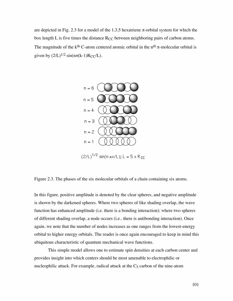
are depicted in Fig. 2.3 for a model of the 1,3,5 hexatriene π-orbital system for which the

box length L is five times the distance RCC between neighboring pairs of carbon atoms.

The magnitude of the kth C-atom centered atomic orbital in the nth π-molecular orbital is

given by (2/L)1/2 sin(nπ(k-1)RCC/L).

Figure 2.3. The phases of the six molecular orbitals of a chain containing six atoms.

In this figure, positive amplitude is denoted by the clear spheres, and negative amplitude

is shown by the darkened spheres. Where two spheres of like shading overlap, the wave

function has enhanced amplitude (i.e. there is a bonding interaction); where two spheres

of different shading overlap, a node occurs (i.e., there is antibonding interaction). Once

again, we note that the number of nodes increases as one ranges from the lowest-energy

orbital to higher energy orbitals. The reader is once again encouraged to keep in mind this

ubiquitous characteristic of quantum mechanical wave functions.

This simple model allows one to estimate spin densities at each carbon center and

provides insight into which centers should be most amenable to electrophilic or

nucleophilic attack. For example, radical attack at the C5 carbon of the nine-atom

102

nonatetraene system described earlier would be more facile for the ground state ψ than

for either ψ* or ψ'*. In the former, the unpaired spin density resides in ψ5 (which varies

as sin(5πx/8RCC) so is non-zero at x = L/2), which has non-zero amplitude at the C5 site

x= L/2 = 4RCC. In ψ* and ψ'*, the unpaired density is in ψ4 and ψ6, respectively, both of

which have zero density at C5 (because sin(nπx/8RCC) vanishes for n = 4 or 6 at x =

4RCC). Plots of the wave functions for n ranging from 1 to 7 are shown in another format

in Fig. 2.4 where the nodal pattern is emphasized.

Figure 2.4. The nodal pattern for a chain containing seven atoms

I hope that by now the student is not tempted to ask how the electron gets from one

region of high amplitude, through a node, to another high-amplitude region. Remember,

such questions are cast in classical Newtonian language and are not appropriate when

103

addressing the wave-like properties of quantum mechanics.

2.2 Bands of Orbitals in Solids

Not only does the particle-in-a-box model offer a useful conceptual representation

of electrons moving in polyenes, but it also is the zeroth-order model of band structures

in solids. Let us consider a simple one-dimensional crystal consisting of a large number

of atoms or molecules, each with a single orbital (the blue spheres shown below) that it

contributes to the bonding. Let us arrange these building blocks in a regular lattice as

shown in the Fig. 2.5.

Figure 2.5. The energy levels arising from 1, 2, 3, 5, and an infinite number of orbitals

In the top four rows of this figure we show the case with 1, 2, 3, and 5 building blocks.

To the left of each row, we display the energy splitting pattern into which the building

blocks’ orbitals evolve as they overlap and form delocalized molecular orbitals. Not

surprisingly, for n = 2, one finds a bonding and an antibonding orbital. For n = 3, one has

a bonding, one non-bonding, and one antibonding orbital. Finally, in the bottom row, we

attempt to show what happens for an infinitely long chain. The key point is that the

discrete number of molecular orbitals appearing in the 1-5 orbital cases evolves into a

continuum of orbitals called a band as the number of building blocks becomes large. This

104

band of orbital energies ranges from its bottom (whose orbital consists of a fully in-phase

bonding combination of the building block orbitals) to its top (whose orbital is a fully

out-of-phase antibonding combination).

In Fig. 2.6 we illustrate these fully bonding and fully antibonding band orbitals

for two cases- the bottom involving s-type building block orbitals, and the top involving

pσ-type orbitals. Notice that when the energy gap between the building block s and pσ

orbitals is larger than is the dispersion (spread) in energy within the band of s or band of

pσ orbitals, a band gap occurs between the highest member of the s band and the lowest

member of the pσ band. The splitting between the s and pσ orbitals is a property of the

individual atoms comprising the solid and varies among the elements of the periodic

table. For example, we teach students that the 2s-2p energy gap in C is smaller than the

3s-3p gap in Si, which is smaller than the 4s-4p gap in Ge. The dispersion in energies that

a given band of orbitals is split into as these atomic orbitals combine to form a band is

determined by how strongly the orbitals on neighboring atoms overlap. Small overlap

produces small dispersion, and large overlap yields a broad band. So, the band structure

of any particular system can vary from one in which narrow bands (weak overlap) do not

span the energy gap between the energies of their constituent atomic orbitals to bands that

overlap strongly (large overlap).

105

Figure 2.6. The bonding through antibonding energies and band orbitals arising from s

and from pσ atomic orbitals.

Depending on how many valence electrons each building block contributes, the

various bands formed by overlapping the building-block orbitals of the constituent atoms

will be filled to various levels. For example, if each building block orbital shown above

has a single valence electron in an s-orbital (e.g., as in the case of the alkali metals), the s-

band will be half filled in the ground state with α and β -paired electrons. Such systems

produce very good conductors because their partially filled s bands allow electrons to

move with very little (e.g., only thermal) excitation among other orbitals in this same

band. On the other hand, for alkaline earth systems with two s electrons per atom, the s-

band will be completely filled. In such cases, conduction requires excitation to the lowest

members of the nearby p-orbital band. Finally, if each building block were an Al (3s2 3p1)

106

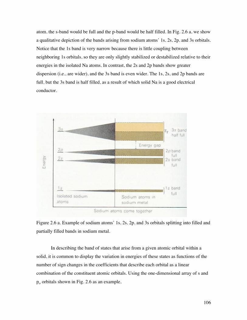
atom, the s-band would be full and the p-band would be half filled. In Fig. 2.6 a, we show

a qualitative depiction of the bands arising from sodium atoms’ 1s, 2s, 2p, and 3s orbitals.

Notice that the 1s band is very narrow because there is little coupling between

neighboring 1s orbitals, so they are only slightly stabilized or destabilized relative to their

energies in the isolated Na atoms. In contrast, the 2s and 2p bands show greater

dispersion (i.e., are wider), and the 3s band is even wider. The 1s, 2s, and 2p bands are

full, but the 3s band is half filled, as a result of which solid Na is a good electrical

conductor.

Figure 2.6 a. Example of sodium atoms’ 1s, 2s, 2p, and 3s orbitals splitting into filled and

partially filled bands in sodium metal.

In describing the band of states that arise from a given atomic orbital within a

solid, it is common to display the variation in energies of these states as functions of the

number of sign changes in the coefficients that describe each orbital as a linear

combination of the constituent atomic orbitals. Using the one-dimensional array of s and

pσ orbitals shown in Fig. 2.6 as an example,

107

(1) the lowest member of the band deriving from the s orbitals

€

φ0 = s(1) + s(2) + s(3) + s(4) + ...+ s(N)

is a totally bonding combination of all of the constituent s orbitals on the N sites of the

lattice.

(2) The highest-energy orbital in this band

€

φN = s(1) − s(2) + s(3) − s(4) + ...+ s(N −1) − s(N)

is a totally anti-bonding combination of the constituent s orbitals.

(3) Each of the intervening orbitals in this band has expansion coefficients that allow the

orbital to be written as

€

φn = cos(n( j −1)πN

)j=1

N

∑ s( j)

Clearly, for small values of n, the series of expansion coefficients

€

cos(n( j −1)πN

)has few

sign changes as the index j runs over the sites of the one-dimensional lattice. For larger n,

there are more sign changes. Thus, thinking of the quantum number n as labeling the

number of sign changes and plotting the energies of the orbitals (on the vertical axis)

versus n (on the horizontal axis), we would obtain a plot that increases from n = 0 to n

=N. In fact, such plots tend to display quadratic variation of the energy with n. This

observation can be understood by drawing an analogy between the pattern of sign

changes belonging to a particular value of n and the number of nodes in the one-

dimensional particle-in-a-box wave function, which also is used to model electronic

states delocalized along a linear chain. As we saw in Chapter 1, the energies for this

model system varied as

108

€

E =j 2π 22

2mL2

with j being the quantum number ranging from 1 to ∞. The lowest-energy state, with j =

1, has no nodes; the state with j = 2 has one node, and that with j = n has (n-1) nodes. So,

if we replace j by (n-1) and replace the box length L by (NR), where R is the inter-atom

spacing and N is the number of atoms in the chain, we obtain

€

E =(n −1)2π 2

2

2mN 2R2

from which on can see why the energy can be expected to vary as (n/N)2.

(4) In contrast for the pσ orbitals, the lowest-energy orbital is

€

φ0 = pσ (1) − pσ (2) + pσ (3) − pσ (4) + ...− pσ (N −1) + pσ (N)

because this alternation in signs allows each

€

pσ orbital on one site to overlap in a bonding

fashion with the

€

pσ orbitals on neighboring sites.

(5) Therefore, the highest-energy orbital in the

€

pσ band is

€

φN = pσ (1) + pσ (2) + pσ (3) + pσ (4) + ...+ pσ (N −1) + pσ (N)

and is totally anti-bonding.

(6) The intervening members of this band have orbitals given by

€

φN−n = cos(n( j −1)πN

)j=1

N

∑ s( j)

with low n corresponding to high-energy orbitals (having few inter-atom sign changes but

anti-bonding character) and high n to low-energy orbitals (having many inter-atom sign

changes). So, in contrast to the case for the s-band orbitals, plotting the energies of the

109

orbitals (on the vertical axis) versus n (on the horizontal axis), we would obtain a plot

that decreases from n = 0 to n =N.

For bands comprised of pπ orbitals, the energies vary with the n quantum number

in a manner analogous to how the s band varies because the orbital with no inter-atom

sign changes is fully bonding. For two- and three-dimensional lattices comprised of s, p,

and d orbitals on the constituent atoms, the behavior of the bands derived from these

orbitals follows analogous trends. It is common to describe the sign alternations arising

from site to site in terms of a so-called k vector. In the one-dimensional case discussed

above, this vector has only one component with elements labeled by the ratio (n/N)

whose value characterizes the number of inter-atom sign changes. For lattices containing

many atoms, N is very large, so n ranges from zero to a very large number. Thus, the

ratio (n/N) ranges from zero to unity in small fractional steps, so it is common to think of

these ratios as describing a continuous parameter varying from zero to one. Moreover, it

is convention to allow the n index to range from –N to +N, so the argument n π /N in the

cosine function introduced above varies from – π to +π.

In two- or three-dimensions the k vector has two or three elements and can be

written in terms of its two or three index ratios, respectively, as

€

k2 = ( nN, mM)

€

k3 = ( nN, mM, lL) .

Here, N, M, and L would describe the number of unit cells along the three principal axes

of the three-dimensional crystal; N and M do likewise in the two-dimensional lattice case.

In such two- and three- dimensional crystal cases, the energies of orbitals within

bands derived from s, p, d, etc. atomic orbitals display variations that also reflect the

number of inter-atom sign changes. However, now there are variations as functions of the

(n/N), (n/M) and (l/L) indices, and these variations can display rather complicated shapes

depending on the symmetry of the atoms within the underlying crystal lattice. That is, as

110

one moves within the three-dimensional space by specifying values of the indices (n/N),

(n/M) and (l/L), one can move throughout the lattice in different symmetry directions. It

is convention in the solid-state literature to plot the energies of these bands as these three

indices vary from site to site along various symmetry elements of the crystal and to

assign a letter to label this symmetry element. The band that has no inter-atom sign

changes is labeled as Γ (sometimes G) in such plots of band structures. In much of our

discussion below, we will analyze the behavior of various bands in the neighborhood of

the Γ point because this is where there are the fewest inter-atom nodes and thus the wave

function is easiest to visualize.

Let’s consider a few examples to help clarify these issues. In Fig. 2.6 b, where we

see the band structure of graphene, you can see the quadratic variations of the energies

with k as one moves away from the k = 0 point labeled Γ, with some bands increasing

with k and others decreasing with k.

Figure 2.6 b Band structure plot for graphene.

The band having an energy of ca. -17 eV at the Γ point originates from bonding

interactions involving 2s orbitals on the carbon atoms, while those having energies near 0

eV at the Γ point derive from carbon 2pσ bonding interactions. The parabolic increase

111

with k for the 2s-based and decrease with k for the 2pσ-based orbitals is clear and is

expected based on our earlier discussion of how s and pσ bands vary with k. The band

having energy near -4 eV at the Γ point involves 2pπ orbitals involved in bonding

interactions, and this band shows a parabolic increase with k as expected as we move

away from the Γ point. These are the delocalized π orbitals of the graphene sheet. The

anti-bonding 2pπ band decreases quadratically with k and has an energy of ca. 15 eV at

the Γ point. Because there are two atoms per unit cell in this case, there are a total of

eight valence electrons (four from each carbon atom) to be accommodated in these bands.

The eight carbon valence electrons fill the bonding 2s and two 2pσ bands fully as well as

the bonding 2pπ band. Only along the direction labeled P in Fig. 2.6 b do the bonding and

anti-bonding 2pπ bands become degenerate (near 2.5 eV); the approach of these two

bands is what allows graphene to be semi-metallic (i.e., to conduct at modest

temperatures- high enough to promote excitations from the bonding 2pπ to the anti-

bonding 2pπ band).

It is interesting to contrast the band structure of graphene with that of diamond,

which is shown in Fig. 2. 6 c.

Figure 2.6 c Band structure of diamond carbon.

112

The band having an energy of ca. – 22 eV at the Γ point derives from 2s bonding

interactions, and the three bands near 0 eV at the Γ point come from 2pσ bonding

interactions. Again, each of these bands displays the expected parabolic behavior as

functions of k. In diamond’s two interpenetrating face centered cubic structure, there are

two carbon atoms per unit cell, so we have a total of eight valence electrons to fill the

four bonding bands. Notice that along no direction in k-space do these filled bonding

bands become degenerate with or are crossed by any of the other bands. The other bands

remain at higher energy along all k-directions, and thus there is a gap between the

bonding bands and the others is large (ca. 5 eV or more along any direction in k-space).

This is why diamond is an insulator; the band gap is very large.

Finally, let’s compare the graphene and diamond cases with a metallic case such

as shown in Fig. 2. 6 d for Al and for Ag.

Figure 2. 6 d Band structures of Al and Ag.

113

For Al and Ag, there is one atom per unit cell, so we have three valence electrons

(3s23p1) and eleven valence electrons (3d10 4s1), respectively, to fill the bands shown in

Fig. 2. 6 d. Focusing on the Γ points in the Al and Ag band structure plots, we can say the

following:

1. For Al, the 3s-based band near -11 eV is filled and the three 3p-based bands near 11

eV have an occupancy of 1/6 (i.e., on average there is one electron in one of these three

bands each of which can hold two electrons).

2. The 3s and 3p bands are parabolic with positive and negative curvature, respectively.

3. Along several directions (e.g. K, W, X, W, L) there are crossings among the bands;

these crossings allow electrons to be promoted from occupied to previously unoccupied

bands. The partial occupancy of the 3p bands and the multiple crossings of bands are

what allow Al to show metallic behavior.

4. For Ag, there are six bands between -4 eV and -8 eV. Five of these bands change little

with k, and one shows somewhat parabolic dependence on k. The former five derive from

4d atomic orbitals that are contracted enough to not allow them to overlap much, and the

latter is based on 5s bonding orbital interaction.

5. Ten of the valence electrons fill the five 4d bands, and the eleventh resides in the 5s-

based bonding band.

6. If the five 4d-based bands are ignored, the remainder of the Ag band structure looks a

lot like that for Al. There are numerous band crossings that include, in particular, the

half-filled 5s band. These crossings and the partial occupancy of the 5s band cause Ag to

have metallic character.

One more feature of band structures that is often displayed is called the band

density of states. An example of such a plot is shown in Fig. 2. 6 e for the TiN crystal.

114

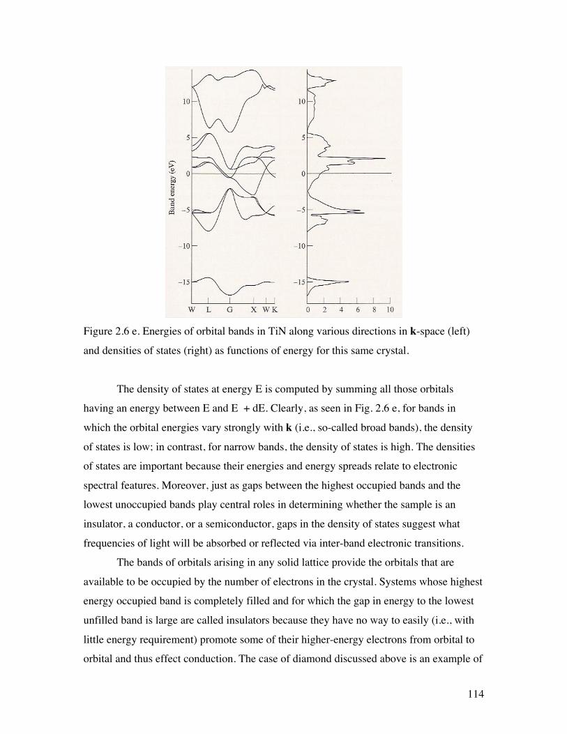
Figure 2.6 e. Energies of orbital bands in TiN along various directions in k-space (left)

and densities of states (right) as functions of energy for this same crystal.

The density of states at energy E is computed by summing all those orbitals

having an energy between E and E + dE. Clearly, as seen in Fig. 2.6 e, for bands in

which the orbital energies vary strongly with k (i.e., so-called broad bands), the density

of states is low; in contrast, for narrow bands, the density of states is high. The densities

of states are important because their energies and energy spreads relate to electronic

spectral features. Moreover, just as gaps between the highest occupied bands and the

lowest unoccupied bands play central roles in determining whether the sample is an

insulator, a conductor, or a semiconductor, gaps in the density of states suggest what

frequencies of light will be absorbed or reflected via inter-band electronic transitions.

The bands of orbitals arising in any solid lattice provide the orbitals that are

available to be occupied by the number of electrons in the crystal. Systems whose highest

energy occupied band is completely filled and for which the gap in energy to the lowest

unfilled band is large are called insulators because they have no way to easily (i.e., with

little energy requirement) promote some of their higher-energy electrons from orbital to

orbital and thus effect conduction. The case of diamond discussed above is an example of

115

an insulator. If the band gap between a filled band and an unfilled band is small, it may

be possible for thermal excitation (i.e., collisions with neighboring atoms or molecules)

to cause excitation of electrons from the former to the latter thereby inducing conductive

behavior. The band structures of Al and Ag discussed above offer examples of this case.

A simple depiction of how thermal excitations can induce conduction is illustrated in Fig.

2.7.

Figure 2.7. The valence and conduction bands and the band gap with a small enough gap

to allow thermal excitation to excite electrons and create holes in a previously filled band.

Systems whose highest-energy occupied band is partially filled are also conductors

because they have little spacing among their occupied and unoccupied orbitals so

electrons can flow easily from one to another. Al and Ag are good examples.

116

To form a semiconductor, one starts with an insulator whose lower band is filled

and whose upper band is empty as shown by the broad bands in Fig.2.8.

Figure 2.8. The filled and empty bands, the band gap, and empty acceptor or filled donor

bands.

If this insulator material is synthesized with a small amount of “dopant” whose valence

orbitals have energies between the filled and empty bands of the insulator, one can

generate a semiconductor. If the dopant species has no valence electrons (i.e., has an

empty valence orbital), it gives rise to an empty band lying between the filled and empty

bands of the insulator as shown below in case a of Fig. 2.8. In this case, the dopant band

can act as an electron acceptor for electrons excited (either thermally or by light) from the

filled band of the insulator into the dopant’s empty band. Once electrons enter the dopant

band, charge can flow (because the insulator’s lower band is no longer filled) and the

system thus becomes a conductor. Another case is illustrated in the b part of Fig. 2.8.

Here, the dopant has a filled band that lies close in energy to the empty band of the

insulator. Excitation of electrons from this dopant band to the insulator’s empty band can

117

induce current to flow (because now the insulator’s upper band is no longer empty).

2.3 Densities of States in 1, 2, and 3 dimensions.

When a large number of neighboring orbitals overlap, bands are formed.

However, the natures of these bands, their energy patterns, and their densities of states

are very different in different dimensions.

Before leaving our discussion of bands of orbitals and orbital energies in solids, I

want to address a bit more the issue of the density of electronic states and what

determines the energy range into which orbitals of a given band will split. First, let’s

recall the energy expression for the 1 and 2- dimensional electron in a box case, and let’s

generalize it to three dimensions. The general result is

E = Σj nj2 π2 h2/(2mLj

2)

where the sum over j runs over the number of dimensions (1, 2, or 3), and Lj is the length

of the box along the jth direction. For one dimension, one observes a pattern of energy

levels that grows with increasing n, and whose spacing between neighboring energy

levels also grows as a result of which the state density decreases with increasing n.

However, in 2 and 3 dimensions, the pattern of energy level spacing displays a

qualitatively different character, especially at high quantum number.

Consider first the 3-dimensional case and, for simplicity, let’s use a box that has

equal length sides L. In this case, the total energy E is (h2π2/2mL2) times (nx2 + ny

2 + nz2).

The latter quantity can be thought of as the square of the length of a vector R having three

components nx, ny, nz. Now think of three Cartesian axes labeled nx, ny, and nz and view a

sphere of radius R in this space. The volume of the 1/8 th sphere having positive values of

nx, ny, and nz and having radius R is 1/8 (4/3 πR3). Because each cube having unit length

along the nx, ny, and nz axes corresponds to a single quantum wave function and its

energy, the total number Ntot(E) of quantum states with positive nx, ny, and nz and with

energy between zero and E = (h2π2/2mL2)R2 is

118

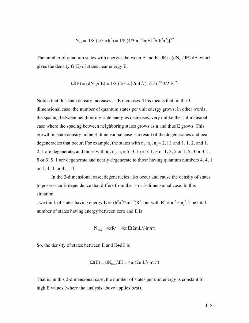
Ntot = 1/8 (4/3 πR3) = 1/8 (4/3 π [2mEL2/( h2π2)]3/2

The number of quantum states with energies between E and E+dE is (dNtot/dE) dE, which

gives the density Ω(E) of states near energy E:

Ω(E) = (dNtot/dE) = 1/8 (4/3 π [2mL2/( h2π2)]3/2 3/2 E1/2.

Notice that this state density increases as E increases. This means that, in the 3-

dimensional case, the number of quantum states per unit energy grows; in other words,

the spacing between neighboring state energies decreases, very unlike the 1-dimensioal

case where the spacing between neighboring states grows as n and thus E grows. This

growth in state density in the 3-dimensional case is a result of the degeneracies and near-

degeneracies that occur. For example, the states with nx, ny, nz = 2,1,1 and 1, 1, 2, and 1,

2, 1 are degenerate, and those with nx, ny, nz = 5, 3, 1 or 5, 1, 3 or 1, 3, 5 or 1, 5, 3 or 3, 1,

5 or 3, 5, 1 are degenerate and nearly degenerate to those having quantum numbers 4, 4, 1

or 1, 4, 4, or 4, 1, 4.

In the 2-dimensional case, degeneracies also occur and cause the density of states

to possess an E-dependence that differs from the 1- or 3-dimensional case. In this

situation

, we think of states having energy E = (h2π2/2mL2)R2, but with R2 = nx2 + ny

2. The total

number of states having energy between zero and E is

Ntotal= 4πR2 = 4π E(2mL2/ h2π2)

So, the density of states between E and E+dE is

Ω(E) = dNtotal/dE = 4π (2mL2/ h2π2)

That is, in this 2-dimensional case, the number of states per unit energy is constant for

high E values (where the analysis above applies best).

119

This kind of analysis for the 1-dimensional case gives

Ntotal= R = (2mEL2/ h2π2)1/2

so, the state density between E and E+ dE is:

Ω(E) = 1/2 (2mL2/ h2π2)1/2 E-1/2,

which clearly shows the widening spacing, and thus lower state density, as one goes to

higher energies.

These findings about densities of states in 1-, 2-, and 3- dimensions are important

because, in various problems one encounters in studying electronic states of extended

systems such as solids, chains, and surfaces, one needs to know how the number of states

available at a given total energy E varies with E. A similar situation occurs when

describing the translational states of an electron or a photo ejected from an atom or

molecule into the vacuum; here the 3-dimensional density of states applies. Clearly, the

state density depends upon the dimensionality of the problem, and this fact is what I want

the students reading this text to keep in mind.

Before closing this Section, it is useful to overview how the various particle-in-

box models can be used as qualitative descriptions for various chemical systems.

1a. The one-dimensional box model is most commonly used to model electronic orbitals

in delocalized linear polyenes.

1b. The electron-on-a-circle model is used to describe orbitals in a conjugated cyclic ring

such as in benzene.

2a. The rectangular box model can be used to model electrons moving within thin layers

of metal deposited on a substrate or to model electrons in aromatic sheets such as

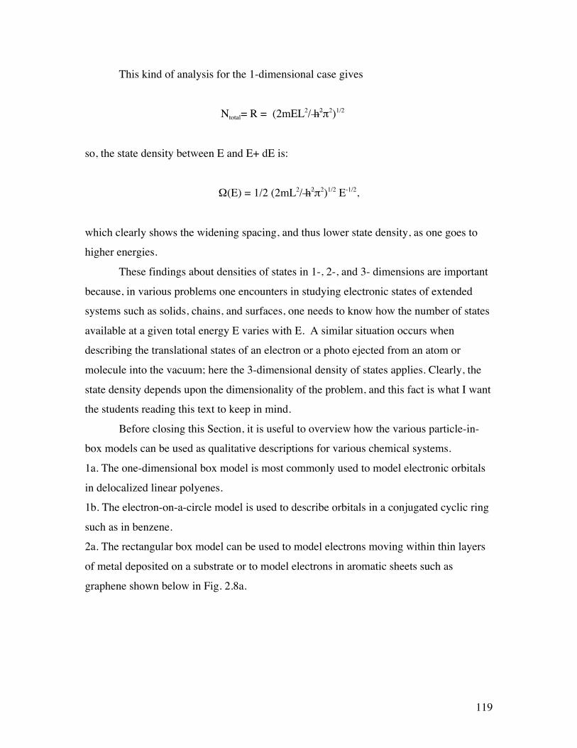
graphene shown below in Fig. 2.8a.

120

Figure 2.8a Depiction of the aromatic rings of graphene extending in two dimensions.

2b. The particle-within-a-circle model can describe states of electrons (or other light

particles requiring quantum treatment) constrained within a circular corral.

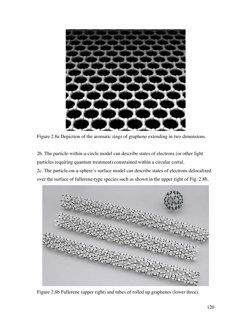
2c. The particle-on-a-sphere’s surface model can describe states of electrons delocalized

over the surface of fullerene-type species such as shown in the upper right of Fig. 2.8b.

Figure 2.8b Fullerene (upper right) and tubes of rolled up graphenes (lower three).

121

3a. The particle-in-a-sphere model, as discussed earlier, is often used to treat electronic

orbitals of quasi-spherical nano-clusters composed of metallic atoms.

3b. The particle-in-a-cube model is often used to describe the bands of electronic orbitals

that arise in three-dimensional crystals constructed from metallic atoms.

In all of these models, the potential V0, which is constant in the region where the electron

is confined, controls the energies of all the quantum states relative to that of a free

electron (i.e., an electron in vacuum with no kinetic energy).

For some dimensionalities and geometries, it may be necessary to invoke more

than one of these models to qualitatively describe the quantum states of systems for

which the valence electrons are highly delocalized (e.g., metallic clusters and conjugated

organics). For example, for electrons residing on the surface of any of the three graphene

tubes shown in Fig. 2.8b, one expects quantum states (i) labeled with an angular

momentum quantum number and characterizing the electrons’ angular motions about the

long axis of the tube, but also (ii) labeled by a long-axis quantum number characterizing

the electron’s energy component along the tube’s long axis. For a three-dimensional tube-

shaped nanoparticle composed of metallic atoms, one expects the quantum states to be (i)

labeled with an angular momentum quantum number and a radial quantum number

characterizing the electrons’ angular motions about the long axis of the tube and its radial

(Bessel function) character, but again also (ii) labeled by a long-axis quantum number

characterizing the electron’s energy component along the tube’s long axis.

2.4 The Most Elementary Model of Orbital Energy Splittings: Hückel or Tight

Binding Theory

Now, let’s examine what determines the energy range into which orbitals (e.g., pπ

orbitals in polyenes, metal, semi-conductor, or insulator; s or pσ orbitals in a solid; or σ or

π atomic orbitals in a molecule) split. I know that, in our earlier discussion, we talked

about the degree of overlap between orbitals on neighboring atoms relating to the energy

splitting, but now it is time to make this concept more quantitative. To begin, consider

two orbitals, one on an atom labeled A and another on a neighboring atom labeled B;

122

these orbitals could be, for example, the 1s orbitals of two hydrogen atoms, such as

Figure 2.9 illustrates.

Figure 2.9. Two 1s orbitals combine to produce a σ bonding and a σ* antibonding

molecular orbital

However, the two orbitals could instead be two pπ orbitals on neighboring carbon atoms

such as are shown in Fig. 2.10 as they form π bonding and π* anti-bonding orbitals.

Figure 2.10. Two atomic pπ orbitals form a bonding π and antibonding π* molecular

orbital.

123

In both of these cases, we think of forming the molecular orbitals (MOs) φk as linear

combinations of the atomic orbitals (AOs) χa on the constituent atoms, and we express

this mathematically as follows:

φK = Σa CK,a χa,

where the CK,a are called linear combination of atomic orbital to form molecular orbital

(LCAO-MO) coefficients. The MOs are supposed to be solutions to the Schrödinger

equation in which the Hamiltonian H involves the kinetic energy of the electron as well

as the potentials VL and VR detailing its attraction to the left and right atomic centers (this

one-electron Hamiltonian is only an approximation for describing molecular orbitals;

more rigorous N-electron treatments will be discussed in Chapter 6):

H = - h2/2m ∇2 + VL + VR.

In contrast, the AOs centered on the left atom A are supposed to be solutions of the

Schrödinger equation whose Hamiltonian is H = - h2/2m ∇2 + VL , and the AOs on the

right atom B have H = - h2/2m ∇2 + VR. Substituting φK = Σa CK,a χa into the MO’s

Schrödinger equation

HφK = εK φK

and then multiplying on the left by the complex conjugate of χb and integrating over the

r, θ and φ coordinates of the electron produces

Σa <χb| - h2/2m ∇2 + VL + VR |χa> CK,a = εK Σa <χb|χa> CK,a

Recall that the Dirac notation <a|b> denotes the integral of a* and b, and <a| op| b>

denotes the integral of a* and the operator op acting on b.

In what is known as the Hückel model in chemistry or the tight-binding model in

124

solid-state theory, one approximates the integrals entering into the above set of linear

equations as follows:

i. The diagonal integral <χb| - h2/2m ∇2 + VL + VR |χb> involving the AO centered on the

right atom and labeled χb is assumed to be equivalent to <χb| - h2/2m ∇2 + VR |χb>, which

means that net attraction of this orbital to the left atomic center is neglected. Moreover,

this integral is approximated in terms of the binding energy (denoted α, not to be

confused with the electron spin function α) for an electron that occupies the χb orbital:

<χb| - h2/2m ∇2 + VR |χb> = αb. The physical meaning of αb is the kinetic energy of the

electron in χb plus the attraction of this electron to the right atomic center while it resides

in χb. Of course, an analogous approximation is made for the diagonal integral involving

χa; <χa| - h2/2m ∇2 + VL |χa> = αa . These α values are negative quantities because, as is

convention in electronic structure theory, energies are measured relative to the energy of

the electron when it is removed from the orbital and possesses zero kinetic energy.

ii. The off-diagonal integrals <χb| - h2/2m ∇2 + VL + VR |χa> are expressed in terms of a

parameter βa,b which relates to the kinetic and potential energy of the electron while it

resides in the “overlap region” in which both χa and χb are non-vanishing. This region is

shown pictorially above as the region where the left and right orbitals touch or overlap.

The magnitude of β is assumed to be proportional to the overlap Sa,b between the two

AOs : Sa,b = <χa|χb>. It turns out that β is usually a negative quantity, which can be seen

by writing it as <χb| - h2/2m ∇2 + VR |χa> + <χb| VL |χa>. Since χa is an eigenfunction of -

h2/2m ∇2 + VR having the eigenvalue αa, the first term is equal to αa (a negative quantity)

times <χb|χa>, the overlap S. The second quantity <χb| VL |χa> is equal to the integral of

the overlap density χb(r) χa(r) multiplied by the (negative) Coulomb potential for

attractive interaction of the electron with the left atomic center. So, whenever χb(r) and

χa(r) have positive overlap, β will turn out negative.

iii. Finally, in the most elementary Hückel or tight-binding model, the off-diagonal

overlap integrals <χa|χb> = Sa,b are neglected and set equal to zero on the right side of the

matrix eigenvalue equation. However, in some Hückel models, overlap between

neighboring orbitals is explicitly treated, so, in some of the discussion below we will

retain Sa,b.

125

With these Hückel approximations, the set of equations that determine the orbital

energies εK and the corresponding LCAO-MO coefficients CK,a are written for the two-

orbital case at hand as in the first 2x2 matrix equations shown below

which is sometimes written as

These equations reduce with the assumption of zero overlap to

The α parameters are identical if the two AOs χa and χb are identical, as would be

the case for bonding between the two 1s orbitals of two H atoms or two 2pπ orbitals of

two C atoms or two 3s orbitals of two Na atoms. If the left and right orbitals were not

identical (e.g., for bonding in HeH+ or for the π bonding in a C-O group), their α values

would be different and the Hückel matrix problem would look like:

To find the MO energies that result from combining the AOs, one must find the

values of ε for which the above equations are valid. Taking the 2x2 matrix consisting of ε

126

times the overlap matrix to the left hand side, the above set of equations reduces to the

third set displayed earlier. It is known from matrix algebra that such a set of linear

homogeneous equations (i.e., having zeros on the right hand sides) can have non-trivial

solutions (i.e., values of C that are not simply zero) only if the determinant of the matrix

on the left side vanishes. Setting this determinant equal to zero gives a quadratic equation

in which the ε values are the unknowns:

(α-ε)2 – (β-εS)2 = 0.

This quadratic equation can be factored into a product

(α - β - ε +εS) (α + β - ε -εS) = 0

which has two solutions

ε = (α + β)/(1 + S), and ε = (α -β)/(1 – S).

As discussed earlier, it turns out that the β values are usually negative, so the

lowest energy such solution is the ε = (α + β)/(1 + S) solution, which gives the energy of

the bonding MO. Notice that the energies of the bonding and anti-bonding MOs are not

symmetrically displaced from the value α within this version of the Hückel model that

retains orbital overlap. In fact, the bonding orbital lies less than β below α, and the

antibonding MO lies more than β above α because of the 1+S and 1-S factors in the

respective denominators. This asymmetric lowering and raising of the MOs relative to the

energies of the constituent AOs is commonly observed in chemical bonds; that is, the

antibonding orbital is more antibonding than the bonding orbital is bonding. This is

another important thing to keep in mind because its effects pervade chemical bonding and

spectroscopy.

Having noted the effect of inclusion of AO overlap effects in the Hückel model, I

should admit that it is far more common to utilize the simplified version of the Hückel

model in which the S factors are ignored. In so doing, one obtains patterns of MO orbital

127

energies that do not reflect the asymmetric splitting in bonding and antibonding orbitals

noted above. However, this simplified approach is easier to use and offers qualitatively

correct MO energy orderings. So, let’s proceed with our discussion of the Hückel model

in its simplified version.

To obtain the LCAO-MO coefficients corresponding to the bonding and

antibonding MOs, one substitutes the corresponding α values into the linear equations

and solves for the Ca coefficients (actually, one can solve for all but one Ca, and then use

normalization of the MO to determine the final Ca). For example, for the bonding MO,

we substitute ε = α + β into the above matrix equation and obtain two equations for CL

and CR:

− β CL + β CR = 0

β CL - β CR = 0.

These two equations are clearly not independent; either one can be solved for one C in

terms of the other C to give:

CL = CR,

which means that the bonding MO is

φ = CL (χL + χR).

The final unknown, CL, is obtained by noting that φ is supposed to be a normalized

function <φ|φ> = 1. Within this version of the Hückel model, in which the overlap S is

neglected, the normalization of φ leads to the following condition:

128

1 = <φ|φ> = CL2 (<χL|χL> + <χRχR>) = 2 CL

2

with the final result depending on assuming that each χ is itself also normalized. So,

finally, we know that CL = (1/2)1/2, and hence the bonding MO is:

φ = (1/2)1/2 (χL + χR).

Actually, the solution of 1 = 2 CL2 could also have yielded CL = - (1/2)1/2 and then, we

would have

φ = - (1/2)1/2 (χL + χR).

These two solutions are not independent (one is just –1 times the other), so only one

should be included in the list of MOs. However, either one is just as good as the other

because, as shown very early in this text, all of the physical properties that one computes

from a wave function depend not on ψ but on ψ*ψ. So, two wave functions that differ

from one another by an overall sign factor as we have here have exactly the same ψ*ψ

and thus are equivalent.

In like fashion, we can substitute ε = α - β into the matrix equation and solve for

the CL can CR values that are appropriate for the antibonding MO. Doing so, gives us:

φ* = (1/2)1/2 (χL - χR)

or, alternatively,

φ* = (1/2)1/2 (χR - χL).

Again, the fact that either expression for φ* is acceptable shows a property of all

solutions to any Schrödinger equations; any multiple of a solution is also a solution. In

the above example, the two answers for φ* differ by a multiplicative factor of (-1).

129

Let’s try another example to practice using Hückel or tight-binding theory. In

particular, I’d like you to imagine two possible structures for a cluster of three Na atoms

(i.e., pretend that someone came to you and asked what geometry you think such a cluster

would assume in its ground electronic state), one linear and one an equilateral triangle.

Further, assume that the Na-Na distances in both such clusters are equal (i.e., that the

person asking for your theoretical help is willing to assume that variations in bond

lengths are not the crucial factor in determining which structure is favored). In Fig. 2.11,

I shown the two candidate clusters and their 3s orbitals.

Figure 2.11. Linear and equilateral triangle structures of sodium trimer.

Numbering the three Na atoms’ valence 3s orbitals χ1, χ2, and χ3, we then set up

the 3x3 Hückel matrix appropriate to the two candidate structures:

for the linear structure (n.b., the zeros arise because χ1 and χ3 do not overlap and thus

have no β coupling matrix element). Alternatively, for the triangular structure, we find

130

as the Hückel matrix. Each of these 3x3 matrices will have three eigenvalues that we

obtain by subtracting ε from their diagonals and setting the determinants of the resulting

matrices to zero. For the linear case, doing so generates

(α-ε)3 – 2 β2 (α-ε) = 0,

and for the triangle case it produces

(α-ε)3 –3 β2 (α-ε) + 2 β2 = 0.

The first cubic equation has three solutions that give the MO energies:

ε = α + (2)1/2 β, ε = α, and ε = α - (2)1/2 β,

for the bonding, non-bonding and antibonding MOs, respectively. The second cubic

equation also has three solutions

ε = α + 2β, ε = α - β , and ε = α - β.

So, for the linear and triangular structures, the MO energy patterns are as shown in Fig.

2.12.

131

Figure 2.12. Energy orderings of molecular orbitals of linear and triangular sodium

trimer.

For the neutral Na3 cluster about which you were asked, you have three valence

electrons to distribute among the lowest available orbitals. In the linear case, we place

two electrons into the lowest orbital and one into the second orbital. Doing so produces a

3-electron state with a total energy of E= 2(α+21/2 β) + α = 3α +2 21/2β. Alternatively, for

the triangular species, we put two electrons into the lowest MO and one into either of the

degenerate MOs resulting in a 3-electron state with total energy E = 3 α + 3β. Because β

is a negative quantity, the total energy of the triangular structure is lower than that of the

linear structure since 3 > 2 21/2.

The above example illustrates how we can use Hückel or tight-binding theory to

make qualitative predictions (e.g., which of two shapes is likely to be of lower energy).

Notice that all one needs to know to apply such a model to any set of atomic orbitals that

overlap to form MOs is

(i) the individual AO energies α (which relate to the electronegativity of the AOs),

(ii) the degree to which the AOs couple (the β parameters which relate to AO overlaps),

(iii) an assumed geometrical structure whose energy one wants to estimate.

This example and the earlier example pertinent to H2 or the π bond in ethylene

also introduce the idea of symmetry. Knowing, for example, that H2, ethylene, and linear

Na3 have a left-right plane of symmetry allows us to solve the Hückel problem in terms

of symmetry-adapted atomic orbitals rather than in terms of primitive atomic orbitals as

we did earlier. For example, for linear Na3, we could use the following symmetry-adapted

functions:

χ2 and (1/2)1/2 {χ1 + χ3}

both of which are even under reflection through the symmetry plane and

(1/2)1/2 {χ1 - χ3}

which is odd under reflection. The 3x3 Hückel matrix would then have the form

132

For example, H1,2 and H2,3 are evaluated as follows

H1,2 = <(1/2)1/2 {χ1 + χ3}|H|χ2> = 2(1/2)1/2 β

Η2,3 = <(1/2)1/2 {χ1 + χ3}|H|<(1/2)1/2 {χ1 - χ3}> = ½{ α + β - β - α} = 0.

The three eigenvalues of the above Hückel matrix are easily seen to be α, α +

€

2β , and

α -

€

2β , exactly as we found earlier. So, it is not necessary to go through the process of

forming symmetry-adapted functions; the primitive Hückel matrix will give the correct

answers even if you do not. However, using symmetry allows us to break the full (3x3 in

this case) Hückel problem into separate Hückel problems for each symmetry component

(one odd function and two even functions in this case, so a 1x1 and a 2x2 sub-matrix).

While we are discussing the issue of symmetry, let me briefly explain the concept

of approximate symmetry again using the above Hückel problem as it applies to ethylene

as an illustrative example.

Figure 2.12a Ethylene molecule’s π and π* orbitals showing the σX,Y reflection plane that

is a symmetry property of this molecule.

€

α 2β 02β α 00 0 α

133

Clearly, as illustrated in Fig. 2.12a, at its equilibrium geometry the ethylene molecule has

a plane of symmetry (denoted σX,Y) that maps nuclei and electrons from its left to its right

and vice versa. This is the symmetry element that could used to decompose the 2x2

Hückel matrix describing the π and π* orbitals into two 1x1 matrices. However, if any of

the four C-H bond lengths or HCH angles is displaced from its equilibrium value in a

manner that destroys the perfect symmetry of this molecule, or if one of the C-H units

were replaced by a C-CH3 unit, it might appear that symmetry would no longer be a

useful tool in analyzing the properties of this molecule’s molecular orbitals. Fortunately,

this is not the case.

Even if there is not perfect symmetry in the nuclear framework of this molecule,

the two atomic pπ orbitals will combine to produce a bonding π and antibonding π*

orbital. Moreover, these two molecular orbitals will still possess nodal properties similar

to those shown in Fig. 2.12a even though they will not possess perfect even and odd

character relative to the σX,Y plane. The bonding orbital will still have the same sign to the

left of the σX,Y plane as it does to the right, and the antibonding orbital will have the

opposite sign to the left as it does to the right, but the magnitudes of these two orbitals

will not be left-right equal. This is an example of the concept of approximate symmetry.

It shows that one can use symmetry, even when it is not perfect, to predict the nodal

patterns of molecular orbitals, and it is the nodal patterns that govern the relative energies

of orbitals as we have seen time and again.

Let’s see if you can do some of this on your own. Using the above results, would

you expect the cation Na3+ to be linear or triangular? What about the anion Na3

-? Next, I

want you to substitute the MO energies back into the 3x3 matrix and find the C1, C2, and

C3 coefficients appropriate to each of the 3 MOs of the linear and of the triangular

structure. See if doing so leads you to solutions that can be depicted as shown in Fig.

2.13, and see if you can place each set of MOs in the proper energy ordering.

134

Figure 2.13. The molecular orbitals of linear and triangular sodium trimer (note, they are

not energy ordered in this figure).

Now, I want to show you how to broaden your horizons and use tight-binding

theory to describe all of the bonds in a more complicated molecule such as ethylene

shown in Fig. 2.14. What is different about this kind of molecule when compared with

metallic or conjugated species is that the bonding can be described in terms of several

pairs of valence orbitals that couple to form two-center bonding and antibonding

molecular orbitals. Within the Hückel model described above, each pair of orbitals that

touch or overlap gives rise to a 2x2 matrix. More correctly, all n of the constituent

valence orbitals form an nxn matrix, but this matrix is broken up into 2x2 blocks. Notice

that this did not happen in the triangular Na3 case where each AO touched two other AOs.

For the ethlyene case, the valence orbitals consist of (a) four equivalent C sp2 orbitals that

are directed toward the four H atoms, (b) four H 1s orbitals, (c) two C sp2 orbitals directed

toward one another to form the C-C σ bond, and (d) two C pπ orbitals that will form the

C-C π bond. This total of 12 orbitals generates 6 Hückel matrices as shown below the

ethylene molecule.

135

Figure 2.14 Ethylene molecule with four C-H bonds, one C-C σ bond, and one C-C π

bond.

We obtain one 2x2 matrix for the C-C σ bond of the form

and one 2x2 matrix for the C-C π bond of the form

Finally, we also obtain four identical 2x2 matrices for the C-H bonds:

136

The above matrices produce (a) four identical C-H bonding MOs having energies ε =

1/2 {(αH + αC) –[(αH-αC)2 + 4β2]1/2}, (b) four identical C-H antibonding MOs having

energies ε* = 1/2 {(αH + αC) + [(αH - αC)2 + 4β2]1/2}, (c) one bonding C-C π orbital with

ε = αpπ + β , (d) a partner antibonding C-C orbital with ε* = αpπ - β, (e) a C-C σ bonding

MO with ε = αsp2 + β , and (f) its antibonding partner with ε* = αsp2 - β. In all of these

expressions, the β parameter is supposed to be that appropriate to the specific orbitals that

overlap as shown in the matrices.

If you wish to practice this exercise of breaking a large molecule down into sets

of interacting valence, try to see what Hückel matrices you obtain and what bonding and

antibonding MO energies you obtain for the valence orbitals of methane shown in Fig.

2.15.

Figure 2.15. Methane molecule with four C-H bonds.

Before leaving this discussion of the Hückel/tight-binding model, I need to stress

that it has its flaws (because it is based on approximations and involves neglecting certain

terms in the Schrödinger equation). For example, it predicts (see above) that ethylene has

four energetically identical C-H bonding MOs (and four degenerate C-H antibonding

MOs). However, this is not what is seen when photoelectron spectra are used to probe the

energies of these MOs. Likewise, it suggests that methane has four equivalent C-H

bonding and antibonding orbitals, which, again is not true. It turns out that, in each of

these two cases (ethylene and methane), the experiments indicate a grouping of four

137

nearly iso-energetic bonding MOs and four nearly iso-energetic antibonding MOs.

However, there is some “splitting” among these clusters of four MOs. The splittings can

be interpreted, within the Hückel model, as arising from couplings or interactions among,

for example, one sp2 or sp3 orbital on a given C atom and another such orbital on the

same atom. Such couplings cause the nxn Hückel matrix to not block-partition into

groups of 2x2 sub-matrices because now there exist off-diagonal β factors that couple

one pair of directed valence to another. When such couplings are included in the analysis,

one finds that the clusters of MOs expected to be degenerate are not but are split just as

the photoelectron data suggest.

2.5 Hydrogenic Orbitals

The Hydrogenic atom problem forms the basis of much of our thinking about

atomic structure. To solve the corresponding Schrödinger equation requires separation

of the r, θ, and φ variables.

The Schrödinger equation for a single particle of mass µ moving in a central

potential (one that depends only on the radial coordinate r) can be written as

-

€

2

2µ∂ 2

∂x2+∂ 2

∂y2+∂ 2

∂z2

ψ + V( )x2+y2+z2 ψ = Eψ.

or, introducing the short-hand notation ∇2:

- h2/2µ ∇2 ψ + V ψ = E ψ.

This equation is not separable in Cartesian coordinates (x,y,z) because of the way x,y,

and z appear together in the square root. However, it is separable in spherical coordinates

where it has the form

€

−2

2µr2∂∂rr2 ∂ψ∂r

-

€

2

2µr21Sinθ

∂∂θ

Sinθ ∂ψ∂θ

138

-

€

2

2µr21

Sin2θ∂ 2ψ∂φ 2 + V(r) ψ = - h2/2µ ∇2 ψ + V ψ = Eψ .

Subtracting V(r) ψ from both sides of the equation and multiplying by - 2µr2

h−2 then

moving the derivatives with respect to r to the right-hand side, one obtains

€

1Sinθ

∂∂θ

Sinθ ∂ψ∂θ

+

€

1Sin2θ

∂ 2ψ∂φ 2

= -

€

2µr2

2 E −V(r)( )ψ -

∂∂r

r2 ∂ψ∂r .

Notice that, except for ψ itself, the right-hand side of this equation is a function of r only;

it contains no θ or φ dependence. Let's call the entire right hand side F(r) ψ to emphasize

this fact.

To further separate the θ and φ dependence, we multiply by Sin2θ and subtract the

θ derivative terms from both sides to obtain

€

∂ 2ψ∂φ 2

= F(r)ψSin2θ - Sinθ

€

∂∂θ

Sinθ ∂ψ∂θ

.

Now we have separated the φ dependence from the θ and r dependence. We now

introduce the procedure used to separate variables in differential equations and assume ψ

can be written as a function of φ times a function of r and θ: ψ = Φ(φ) Q(r,θ). Dividing by

Φ Q, we obtain

139

1Φ

€

∂ 2Φ∂φ 2

=

€

1QF(r)Sin2θQ −Sinθ ∂

∂θSinθ ∂Q

∂θ

.

Now all of the φ dependence is isolated on the left hand side; the right hand side contains

only r and θ dependence.

Whenever one has isolated the entire dependence on one variable as we have done

above for the φ dependence, one can easily see that the left and right hand sides of the

equation must equal a constant. For the above example, the left hand side contains no r

or θ dependence and the right hand side contains no φ dependence. Because the two

sides are equal for all values of r, θ, and φ, they both must actually be independent of r, θ,

and φ dependence; that is, they are constant. This again is what is done when one

employs the separations of variables method in partial differential equations.

For the above example, we therefore can set both sides equal to a so-called

separation constant that we call -m2. It will become clear shortly why we have chosen to

express the constant in the form of minus the square of an integer. You may recall that we

studied this same φ - equation earlier and learned how the integer m arises via. the

boundary condition that φ and φ + 2π represent identical geometries.

2.5.1. The Φ Equation

The resulting Φ equation reads (the “ symbol is used to represent second

derivative)

Φ" + m2Φ = 0.

This equation should be familiar because it is the equation that we treated much earlier

when we discussed z-component of angular momentum. So, its further analysis should

also be familiar, but for completeness, I repeat much of it. The above equation has as its

140

most general solution

Φ = Α eimφ + B e-imφ .

Because the wave functions of quantum mechanics represent probability densities, they

must be continuous and single-valued. The latter condition, applied to our Φ function,

means (n.b., we used this in our earlier discussion of z-component of angular momentum)

that

Φ(φ) = Φ(2π + φ) or,

Aeimφ( )1 - e2imπ + Be-imφ( )1 - e-2imπ = 0.

This condition is satisfied only when the separation constant is equal to an integer m = 0,

±1, ± 2, ... . and provides another example of the rule that quantization comes from the

boundary conditions on the wave function. Here m is restricted to certain discrete values

because the wave function must be such that when you rotate through 2π about the z-axis,

you must get back what you started with.

2.5.2. The Θ Equation

Now returning to the equation in which the φ dependence was isolated from the r

and θ dependence and rearranging the θ terms to the left-hand side, we have

€

1Sinθ

∂∂θ

Sinθ ∂Q∂θ

-

€

m2QSin2θ

= F(r)Q.

141

In this equation we have separated the θ and r terms, so we can further decompose the

wave function by introducing Q = Θ(θ) R(r) , which yields

€

1Θ

1Sinθ

∂∂θ

Sinθ ∂Θ∂θ

-

m2

Sin2θ = F(r)R

R = -λ,

where a second separation constant, -λ, has been introduced once the r and θ dependent

terms have been separated onto the right and left hand sides, respectively.

We now can write the θ equation as

€

1Sinθ

∂∂θ

Sinθ ∂Θ∂θ

-

m2ΘSin2θ = -λ Θ,

where m is the integer introduced earlier. To solve this equation for Θ, we make the

substitutions z = Cosθ and P(z) = Θ(θ) , so 1-z2 = Sinθ , and

€

∂∂θ

=

€

∂z∂θ

∂∂z

= - Sinθ

€

∂∂z

.

The range of values for θ was 0 ≤ θ < π , so the range for z is -1 < z < 1. The equation

for Θ, when expressed in terms of P and z, becomes

€

ddz

(1− z2) dPdz

-

m2P1-z2 + λP = 0.

Now we can look for polynomial solutions for P, because z is restricted to be less than

142

unity in magnitude. If m = 0, we first let

P =

€

akzk

k= 0∑ ,

and substitute into the differential equation to obtain

€

(k + 2)(k + 1)ak+2zk

k= 0∑ -

€

(k + 1)k akzk

k= 0∑ + λ

€

akzk

k= 0∑ = 0.

Equating like powers of z gives

ak+2 = ak(k(k+1)-λ)(k+2)(k+1) .

Note that for large values of k

ak+2ak

→ k2

1+1k

k2

1+2k

1+1k

= 1.

Since the coefficients do not decrease with k for large k, this series will diverge for z = ±

1 unless it truncates at finite order. This truncation only happens if the separation

constant λ obeys λ = l(l+1), where l is an integer (you can see this from the recursion

relation giving ak+2 in terms of ak; only for certain values of λ will the numerator vanish ).

So, once again, we see that a boundary condition (i.e., that the wave function not diverge

and thus be normalizable in this case) give rise to quantization. In this case, the values of

λ are restricted to l(l+1); before, we saw that m is restricted to 0, ±1, ± 2, .. .

Since the above recursion relation links every other coefficient, we can choose to

solve for the even and odd functions separately. Choosing a0 and then determining all of

the even ak in terms of this a0, followed by rescaling all of these ak to make the function

143

normalized generates an even solution. Choosing a1 and determining all of the odd ak in

like manner, generates an odd solution.

For l= 0, the series truncates after one term and results in Po(z) = 1. For l= 1 the

same thing applies and P1(z) = z. For l= 2, a2 = -6 ao2 = -3ao, so one obtains P2 = 3z2-1,

and so on. These polynomials are called Legendre polynomials and are denoted Pl(z).

For the more general case where m ≠ 0, one can proceed as above to generate a

polynomial solution for the Θ function. Doing so, results in the following solutions:

€

Plm (z) = (1− z2)|m | / 2 d

|m |Pl (z)dz|m |

These functions are called Associated Legendre polynomials, and they constitute the

solutions to the Θ problem for non-zero m values.

The above P and eimφ functions, when re-expressed in terms of θ and φ, yield the

full angular part of the wave function for any centrosymmetric potential. These solutions

are usually written as

Yl,m(θ,φ)=

€

P lm(cosθ) (2π)-1/2 exp(imφ),

and are called spherical harmonics. They provide the angular solution of the r,θ, φ

Schrödinger equation for any problem in which the potential depends only on the radial

coordinate. Such situations include all one-electron atoms and ions (e.g., H, He+, Li++,

etc.), the rotational motion of a diatomic molecule (where the potential depends only on

bond length r), the motion of a nucleon in a spherically symmetrical box (as occurs in the

shell model of nuclei), and the scattering of two atoms (where the potential depends only

on interatomic distance).

The Yl,m functions possess varying number of angular nodes, which, as noted

144

earlier, give clear signatures of the angular or rotational energy content of the wave

function. These angular nodes originate in the oscillatory nature of the Legendre and

associated Legendre polynomials Plm

(cosθ); the higher l is, the more sign changes occur

within the polynomial.

2.5.3. The R Equation

Let us now turn our attention to the radial equation, which is the only place that

the explicit form of the potential appears. Using our earlier results for the equation

obeyed by the R(r) function and specifying V(r) to be the Coulomb potential appropriate

for an electron in the field of a nucleus of charge +Ze, yields:

€

1r2ddr

r2 dRdr

+

€

2µ2 E +

Ze2

r

−

L(L + 1)r2

R = 0.

We can simplify things considerably if we choose rescaled length and energy units

because doing so removes the factors that depend on µ, h− , and e. We introduce a new

radial coordinate ρ and a quantity σ as follows:

€

ρ = r −8µE2

1/ 2

and σ =

€

µZe2

−2µE.

Notice that if E is negative, as it will be for bound states (i.e., those states with energy

below that of a free electron infinitely far from the nucleus and with zero kinetic energy),

ρ and σ are real. On the other hand, if E is positive, as it will be for states that lie in the

continuum, ρ and σ will be imaginary. These two cases will give rise to qualitatively

different behavior in the solutions of the radial equation developed below.

We now define a function S such that S(ρ) = R(r) and substitute S for R to obtain:

145

€

1ρ2ddρ

ρ2dSdρ

+

€

−14−L(L + 1)ρ2

+σρ

S = 0.

The differential operator terms can be recast in several ways using

€

1ρ2ddρ

ρ2 dSdρ

=

€

d2Sdρ2

+

€

2ρdSdρ

=

€

1ρd2

dρ2(ρS) .

The strategy that we now follow is characteristic of solving second order differential

equations. We will examine the equation for S at large and small ρ values. Having

found solutions at these limits, we will use a power series in ρ to interpolate between

these two limits.

Let us begin by examining the solution of the above equation at small values of ρ

to see how the radial functions behave at small r. As ρ→0, the term -L(L+1)/ρ 2 will

dominate over -1/4 +σ/ρ. Neglecting these other two terms, we find that, for small values

of ρ (or r), the solution should behave like ρL and because the function must be

normalizable, we must have L ≥ 0. Since l can be any non-negative integer, this suggests

the following more general form for S(ρ) :

S(ρ) ≈ ρL e-aρ.

This form will insure that the function is normalizable since S(ρ) → 0 as r → ∞ for all L,

as long as ρ is a real quantity. If ρ is imaginary, such a form may not be normalized (see

below for further consequences).

Turning now to the behavior of S for large ρ, we make the substitution of S(ρ)

into the above equation and keep only the terms with the largest power of ρ (i.e., the -1/4

term) and we allow the derivatives in the above differential equation to act on ≈ ρL e-aρ.

Upon so doing, we obtain the equation

146

a2ρLe-aρ = 14 ρLe-aρ ,

which leads us to conclude that the exponent in the large-ρ behavior of S is a = 12 .

Having found the small-ρ and large-ρ behaviors of S(ρ), we can take S to have the

following form to interpolate between large and small ρ-values:

S(ρ) = ρLe-ρ2 P(ρ),

where the function P is expanded in an infinite power series in ρ as P(ρ) = ∑ak ρk .

Again substituting this expression for S into the above equation we obtain

P"ρ + P'(2L+2-ρ) + P(σ-L-l) = 0,

and then substituting the power series expansion of P and solving for the ak's we arrive at

a recursion relation for the ak coefficients:

ak+1 =

€

(k −σ + L + l)ak(k + 1)(k + 2L + 2)

.

For large k, the ratio of expansion coefficients reaches the limit ak+1ak

= 1k , which, when

substituted into ∑ak ρk , gives the same behavior as the power series expansion of eρ.

Because the power series expansion of P describes a function that behaves like eρ for

147

large ρ, the resulting S(ρ) function would not be normalizable because the e-ρ2 factor

would be overwhelmed by this eρ dependence. Hence, the series expansion of P must

truncate in order to achieve a normalizable S function. Notice that if ρ is imaginary, as it

will be if E is in the continuum, the argument that the series must truncate to avoid an

exponentially diverging function no longer applies. Thus, we see a key difference

between bound (with ρ real) and continuum (with ρ imaginary) states. In the former

case, the boundary condition of non-divergence arises; in the latter, it does not because

exp(ρ/2) does not diverge if ρ is imaginary.

To truncate at a polynomial of order n', we must have n' - σ + L+ l= 0. This

implies that the quantity σ introduced previously is restricted to σ = n' + L + l, which is

certainly an integer; let us call this integer n. If we label states in order of increasing n =

1,2,3,... , we see that doing so is consistent with specifying a maximum order (n') in the

P(ρ) polynomial n' = 0,1,2,... after which the L-value can run from L = 0, in steps of unity

up to L = n-1.

Substituting the integer n for σ, we find that the energy levels are quantized

because σ is quantized (equal to n):

E = -

€

µZ2e4

22n2

and the scaled distance turns out to be

ρ =

€

Zraon

.

Here, the length ao is the so-called Bohr radius

€

ao =2

µe2

, which turns out to be 0.529

Å; it appears once the above E-expression is substituted into the equation for ρ. Using

the recursion equation to solve for the polynomial's coefficients ak for any choice of n

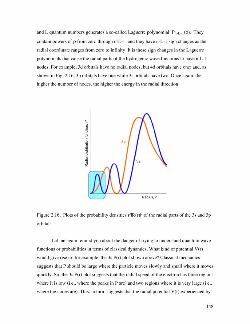
148

and L quantum numbers generates a so-called Laguerre polynomial; Pn-L-1(ρ). They

contain powers of ρ from zero through n-L-1, and they have n-L-1 sign changes as the

radial coordinate ranges from zero to infinity. It is these sign changes in the Laguerre

polynomials that cause the radial parts of the hydrogenic wave functions to have n-L-1

nodes. For example, 3d orbitals have no radial nodes, but 4d orbitals have one; and, as

shown in Fig. 2.16, 3p orbitals have one while 3s orbitals have two. Once again, the

higher the number of nodes, the higher the energy in the radial direction.

Figure 2.16. Plots of the probability densities r2|R(r)|2 of the radial parts of the 3s and 3p

orbitals

Let me again remind you about the danger of trying to understand quantum wave

functions or probabilities in terms of classical dynamics. What kind of potential V(r)

would give rise to, for example, the 3s P(r) plot shown above? Classical mechanics

suggests that P should be large where the particle moves slowly and small where it moves

quickly. So, the 3s P(r) plot suggests that the radial speed of the electron has three regions

where it is low (i.e., where the peaks in P are) and two regions where it is very large (i.e.,

where the nodes are). This, in turn, suggests that the radial potential V(r) experienced by

149

the 3s electron is high in three regions (near peaks in P) and low in two regions. Of

course, this conclusion about the form of V(r) is nonsense and again illustrates how one

must not be drawn into trying to think of the classical motion of the particle, especially

for quantum states with small quantum number. In fact, the low quantum number states

of such one-electron atoms and ions have their radial P(r) plots focused in regions of r-

space where the potential –Ze2/r is most attractive (i.e., largest in magnitude).

Finally, we note that the energy quantization does not arise for states lying in the

continuum because the condition that the expansion of P(ρ) terminate does not arise. The

solutions of the radial equation appropriate to these scattering states (which relate to the

scattering motion of an electron in the field of a nucleus of charge Z) are a bit outside the

scope of this text, so we will not treat them further here. For the interested student, they

are treated on p. 90 of the text by Eyring, Walter, and Kimball to which I refer in the

Introductory Remarks to this text.

To review, separation of variables has been used to solve the full r,θ,φ

Schrödinger equation for one electron moving about a nucleus of charge Z. The θ and φ

solutions are the spherical harmonics YL,m (θ,φ). The bound-state radial solutions

Rn,L(r) = S(ρ) = ρLe-ρ2 Pn-L-1(ρ)

depend on the n and L quantum numbers and are given in terms of the Laguerre

polynomials.

2.5.4. Summary

To summarize, the quantum numbers L and m arise through boundary conditions

requiring that ψ(θ) be normalizable (i.e., not diverge) and ψ(φ) = ψ(φ+2π). The radial

equation, which is the only place the potential energy enters, is found to possess both

bound-states (i.e., states whose energies lie below the asymptote at which the potential

vanishes and the kinetic energy is zero) and continuum states lying energetically above

this asymptote. The former states are spatially confined by the potential, but the latter are

not. The resulting hydrogenic wave functions (angular and radial) and energies are

150

summarized on pp. 133-136 in the text by L. Pauling and E. B. Wilson for n up to and

including 6 and L up to 5 (i.e, for s, p, d, f, g, and h orbitals).

There are both bound and continuum solutions to the radial Schrödinger equation

for the attractive coulomb potential because, at energies below the asymptote, the

potential confines the particle between r=0 and an outer classical turning point, whereas

at energies above the asymptote, the particle is no longer confined by an outer turning

point (see Fig. 2.17). This provides yet another example of how quantized states arise

when the potential spatially confines the particle, but continuum states arise when the

particle is not spatially confined.

Figure 2.17. Radial Potential for Hydrogenic Atoms and Bound and Continuum Orbital

Energies.

The solutions of this one-electron problem form the qualitative basis for much of atomic

and molecular orbital theory. For this reason, the reader is encouraged to gain a firmer

understanding of the nature of the radial and angular parts of these wave functions. The

orbitals that result are labeled by n, l, and m quantum numbers for the bound states and

by l and m quantum numbers and the energy E for the continuum states. Much as the

151

particle-in-a-box orbitals are used to qualitatively describe π- electrons in conjugated

polyenes, these so-called hydrogen-like orbitals provide qualitative descriptions of

orbitals of atoms with more than a single electron. By introducing the concept of

screening as a way to represent the repulsive interactions among the electrons of an atom,

an effective nuclear charge Zeff can be used in place of Z in the ψn,l,m and En to generate

approximate atomic orbitals to be filled by electrons in a many-electron atom. For

example, in the crudest approximation of a carbon atom, the two 1s electrons experience

the full nuclear attraction so Zeff = 6 for them, whereas the 2s and 2p electrons are

screened by the two 1s electrons, so Zeff = 4 for them. Within this approximation, one then

occupies two 1s orbitals with Z = 6, two 2s orbitals with Z = 4 and two 2p orbitals with

Z=4 in forming the full six-electron wave function of the lowest-energy state of carbon. It

should be noted that the use of screened nuclear charges as just discussed is different

from the use of a quantum defect parameter δ as discussed regarding Rydberg orbitals in

Chapter 1. The Z = 4 screened charge for carbon’s 2s and 2p orbitals is attempting to

represent the effect of the inner-shell 1s electrons on the 2s and 2p orbitals. The

modification of the principal quantum number made by replacing n by (n- δ) represents

the penetration of the orbital with nominal quantum number n inside its inner-shells.

2.6. Electron Tunneling

Tunneling is a phenomenon of quantum mechanics, not classical mechanics. It is

an extremely important subject that occurs in a wide variety of chemical species

including nano-scale electronic devices and protons moving through water.

As we have seen several times already, solutions to the Schrödinger equation

display several properties that are very different from what one experiences in Newtonian

dynamics. One of the most unusual and important is that the particles one describes using

quantum mechanics can move into regions of space where they would not be allowed to

go if they obeyed classical equations. We call these classically forbidden regions. Let us

consider an example to illustrate this so-called tunneling phenomenon. Specifically, we

think of an electron (a particle that we likely would use quantum mechanics to describe)

moving in a direction we will call R under the influence of a potential that is:

152

a. Infinite for R < 0 (this could, for example, represent a region of space within a solid

material where the electron experiences very repulsive interactions with other electrons);

b. Constant and negative for some range of R between R = 0 and Rmax (this could

represent the attractive interaction of the electrons with those atoms or molecules in a

finite region or surface of a solid);

c. Constant and repulsive (i.e., positive) by an amount δV + De for another finite region

from Rmax to Rmax +δ (this could represent the repulsive interactions between the electrons

and a layer of molecules of thickness δ lying on the surface of the solid at Rmax);

d. Constant and equal to De from Rmaz +δ to infinity (this could represent the electron

being removed from the solid, but with a work function energy cost of De, and moving

freely in the vacuum above the surface and the ad-layer). Such a potential is shown in

Fig. 2.18.

Figure 2.18. One-dimensional potential showing a well, a barrier, and the asymptotic

region.

153

The piecewise nature of this potential allows the one-dimensional Schrödinger equation

to be solved analytically. For energies lying in the range De < E < De +δV, an especially

interesting class of solutions exists. These so-called resonance states occur at energies

that are determined by the condition that the amplitude of the wave function within the

barrier (i.e., for 0 ≤ R ≤ Rmax ) be large. Let us now turn our attention to this specific

energy regime, which also serves to introduce the tunneling phenomenon.

The piecewise solutions to the Schrödinger equation appropriate to the resonance

case are easily written down in terms of sin and cos or exponential functions, using the

following three definitions:

The combination of sin(kR) and cos(kR) that solve the Schrödinger equation in the inner

region and that vanish at R=0 (because the function must vanish within the region where

V is infinite and because it must be continuous, it must vanish at R=0) is:

ψ = Asin(kR) (for 0 ≤ R ≤ Rmax ).

Between Rmax and Rmax +δ, there are two solutions that obey the Schrödiger equation, so

the most general solution is a combination of these two:

ψ = B+ exp(κ'R) + B- exp(-κ'R) (for Rmax ≤ R ≤ Rmax +δ).

Finally, in the region beyond Rmax + δ, we can use a combination of either sin(k’R) and

cos(k’R) or exp(ik’R) and exp(-ik’R) to express the solution. Unlike the region near R=0,

where it was most convenient to use the sin and cos functions because one of them could

be “thrown away” since it could not meet the boundary condition of vanishing at R=0, in

this large-R region, either set is acceptable. We choose to use the exp(ik’R) and

€

k = 2meE /2 ,k'= 2me (E −De ) /

2 ,κ '= 2me (De + δV − E) /2

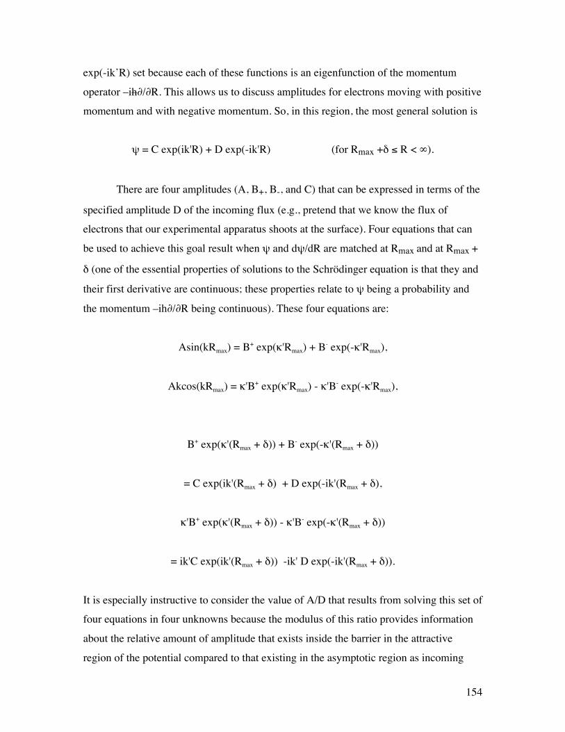
154

exp(-ik’R) set because each of these functions is an eigenfunction of the momentum

operator –ih∂/∂R. This allows us to discuss amplitudes for electrons moving with positive

momentum and with negative momentum. So, in this region, the most general solution is

ψ = C exp(ik'R) + D exp(-ik'R) (for Rmax +δ ≤ R < ∞).

There are four amplitudes (A, B+, B-, and C) that can be expressed in terms of the

specified amplitude D of the incoming flux (e.g., pretend that we know the flux of

electrons that our experimental apparatus shoots at the surface). Four equations that can

be used to achieve this goal result when ψ and dψ/dR are matched at Rmax and at Rmax +

δ (one of the essential properties of solutions to the Schrödinger equation is that they and

their first derivative are continuous; these properties relate to ψ being a probability and

the momentum –ih∂/∂R being continuous). These four equations are:

Asin(kRmax) = B+ exp(κ'Rmax) + B- exp(-κ'Rmax),

Akcos(kRmax) = κ'B+ exp(κ'Rmax) - κ'B- exp(-κ'Rmax),

B+ exp(κ'(Rmax + δ)) + B- exp(-κ'(Rmax + δ))

= C exp(ik'(Rmax + δ) + D exp(-ik'(Rmax + δ),

κ'B+ exp(κ'(Rmax + δ)) - κ'B- exp(-κ'(Rmax + δ))

= ik'C exp(ik'(Rmax + δ)) -ik' D exp(-ik'(Rmax + δ)).

It is especially instructive to consider the value of A/D that results from solving this set of

four equations in four unknowns because the modulus of this ratio provides information

about the relative amount of amplitude that exists inside the barrier in the attractive

region of the potential compared to that existing in the asymptotic region as incoming

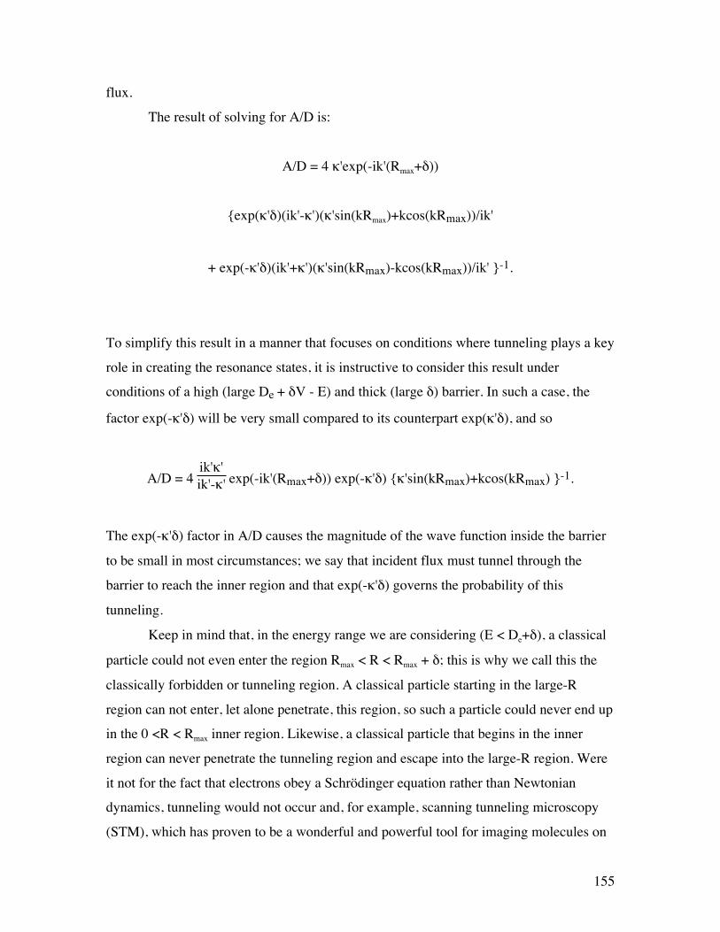
155

flux.

The result of solving for A/D is:

A/D = 4 κ'exp(-ik'(Rmax+δ))

{exp(κ'δ)(ik'-κ')(κ'sin(kRmax)+kcos(kRmax))/ik'

+ exp(-κ'δ)(ik'+κ')(κ'sin(kRmax)-kcos(kRmax))/ik' }-1.

To simplify this result in a manner that focuses on conditions where tunneling plays a key

role in creating the resonance states, it is instructive to consider this result under

conditions of a high (large De + δV - E) and thick (large δ) barrier. In such a case, the

factor exp(-κ'δ) will be very small compared to its counterpart exp(κ'δ), and so

A/D = 4 ik'κ'ik'-κ' exp(-ik'(Rmax+δ)) exp(-κ'δ) {κ'sin(kRmax)+kcos(kRmax) }-1.

The exp(-κ'δ) factor in A/D causes the magnitude of the wave function inside the barrier

to be small in most circumstances; we say that incident flux must tunnel through the

barrier to reach the inner region and that exp(-κ'δ) governs the probability of this

tunneling.

Keep in mind that, in the energy range we are considering (E < De+δ), a classical

particle could not even enter the region Rmax < R < Rmax + δ; this is why we call this the

classically forbidden or tunneling region. A classical particle starting in the large-R

region can not enter, let alone penetrate, this region, so such a particle could never end up

in the 0 <R < Rmax inner region. Likewise, a classical particle that begins in the inner

region can never penetrate the tunneling region and escape into the large-R region. Were

it not for the fact that electrons obey a Schrödinger equation rather than Newtonian

dynamics, tunneling would not occur and, for example, scanning tunneling microscopy

(STM), which has proven to be a wonderful and powerful tool for imaging molecules on

156

and near surfaces, would not exist. Likewise, many of the devices that appear in our

modern electronic tools and games, which depend on currents induced by tunneling

through various junctions, would not be available. But, or course, tunneling does occur

and it can have remarkable effects.

Let us examine an especially important (in chemistry) phenomenon that takes

place because of tunneling and that occurs when the energy E assumes very special

values. The magnitude of the A/D factor in the above solutions of the Schrödinger

equation can become large if the energy E is such that the denominator in the above

expression for A/D approaches zero. This happens when

κ'sin(kRmax)+kcos(kRmax)

or if

tan(kRmax) = - k/κ’.

It can be shown that the above condition is similar to the energy quantization

condition

tan(kRmax) = - k/κ

that arises when bound states of a finite potential well similar to that shown above but

with the barrier between Rmax and Rmax + δ missing and with E below De. There is,

however, a difference. In the bound-state situation, two energy-related parameters occur

k = 2µE/h2

and

κ = 2µ(De - E)/h2 .

157

In the case we are now considering, k is the same, but

κ' = 2µ(De +δV - E)/h2 )

rather than κ occurs, so the two equations involving tan(kRmax) are not identical, but they

are quite similar.

Another observation that is useful to make about the situations in which A/D

becomes very large can be made by considering the case of a very high barrier (so that κ'

is much larger than k). In this case, the denominator that appears in A/D

κ'sin(kRmax)+kcos(kRmax) ≅ κ' sin(kRmax)

can become small at energies satisfying

sin(kRmax) ≅ 0.

This condition is nothing but the energy quantization condition that occurs for the

particle-in-a-box potential shown in Fig. 2.19.

Figure 2.19. One-dimensional potential similar to the tunneling potential but without the

barrier and asymptotic region.

158

This potential is identical to the potential that we were examining for 0 ≤ R ≤ Rmax , but

extends to infinity beyond Rmax ; the barrier and the dissociation asymptote displayed by

our potential are absent.

Let’s consider what this tunneling problem has taught us. First, it showed us that

quantum particles penetrate into classically forbidden regions. It showed that, at certain

so-called resonance energies, tunneling is much more likely than at energies that are off-

resonance. In our model problem, this means that electrons impinging on the surface with

resonance kinetic energies will have a very high probability of tunneling to produce an

electron that is highly localized (i.e., trapped) in the 0 < R < Rmax region. Likewise, it

means that an electron prepared (e.g., perhaps by photo-excitation from a lower-energy

electronic state) within the 0 < R < Rmax region will remain trapped in this region for a

long time (i.e., will have a low probability of tunneling outward).

In the case just mentioned, it would make sense to solve the four equations for the

amplitude C of the outgoing wave in the R > Rmax region in terms of the A amplitude. If

we were to solve for C/A and then examine under what conditions the amplitude of this

ratio would become small (so the electron cannot escape), we would find the same

tan(kRmax) = - k/κ' resonance condition as we found from the other point of view. This

means that the resonance energies tell us for what collision energies the electron will

tunnel inward and produce a trapped electron and, at these same energies, an electron that

is trapped will not escape quickly.

Whenever one has a barrier on a potential energy surface, at energies above the

dissociation asymptote De but below the top of the barrier (De + δV here), one can expect

resonance states to occur at special scattering energies E. As we illustrated with the

model problem, these so-called resonance energies can often be approximated by the

bound-state energies of a potential that is identical to the potential of interest in the inner

region (0 ≤ R ≤ Rmax ) but that extends to infinity beyond the top of the barrier (i.e.,

beyond the barrier, it does not fall back to values below E).

The chemical significance of resonances is great. Highly rotationally excited

molecules may have more than enough total energy to dissociate (De), but this energy

may be stored in the rotational motion, and the vibrational energy may be less than De. In

159

terms of the above model, high rotational angular momentum may produce a significant

centrifugal barrier in the effective potential that characterizes the molecule’s vibration,

but the system's vibrational energy may lie significantly below De. In such a case, and

when viewed in terms of motion on an angular-momentum-modified effective potential

such as I show in Fig. 2.20 , the lifetime of the molecule with respect to dissociation is

determined by the rate of tunneling through the barrier.

Figure 2.20. Radial potential for non-rotating (J = 0) molecule and for rotating molecule.

In this case, one speaks of rotational predissociation of the molecule. The lifetime

τ can be estimated by computing the frequency ν at which flux that exists inside Rmax

strikes the barrier at Rmax

ν = hk

2µRmax (sec-1)

160

and then multiplying by the probability P that flux tunnels through the barrier from Rmax

to Rmax + δ:

P = exp(-2κ'δ).

The result is that

τ -1= hk

2µRmax exp(-2κ'δ)

with the energy E entering into k and κ' being determined by the resonance condition:

(κ'sin(kRmax)+kcos(kRmax)) = minimum. We note that the probability of tunneling exp(-

2κ'δ) falls of exponentially with a factor depending on the width δ of the barrier through

which the particle must tunnel multiplied by κ’, which depends on the height of the

barrier De + δ above the energy E available. This exponential dependence on thickness

and height of the barriers is something you should keep in mind because it appears in all

tunneling rate expressions.

Another important case in which tunneling occurs is in electronically metastable

states of anions. In so-called shape resonance states, the anion’s extra electron

experiences

a. an attractive potential due to its interaction with the underlying neutral molecule’s

dipole, quadrupole, and induced electrostatic moments, as well as

b. a centrifugal potential of the form L(L+1)h2/8π2meR2 whose magnitude depends on

the angular character of the orbital the extra electron occupies.

When combined, the above attractive and centrifugal potentials produce an effective

radial potential of the form shown in Fig. 2.21 for the N2- case in which the added

electron occupies the π* orbital which has L=2 character when viewed from the center of

the N-N bond. Again, tunneling through the barrier in this potential determines the

lifetimes of such shape resonance states.

161

Figure 2.21 Effective radial potential for the excess electron in N2- occupying the π*

orbital which has a dominant L = 2 component.

Although the examples treated above analytically involved piecewise constant

potentials (so the Schrödinger equation and the boundary matching conditions could be

solved exactly), many of the characteristics observed carry over to more chemically

realistic situations. In fact, one can often model chemical reaction processes in terms of

motion along a reaction coordinate (s) from a region characteristic of reactant materials

where the potential surface is positively curved in all direction and all forces (i.e.,

gradients of the potential along all internal coordinates) vanish; to a transition state at

which the potential surface's curvature along s is negative while all other curvatures are

positive and all forces vanish; onward to product materials where again all curvatures are

positive and all forces vanish. A prototypical trace of the energy variation along such a

reaction coordinate is in Fig. 2.22.

162

Figure 2.22. Energy profile along a reaction path showing the barrier through which

tunneling may occur.

Near the transition state at the top of the barrier on this surface, tunneling through the

barrier plays an important role if the masses of the particles moving in this region are

sufficiently light. Specifically, if H or D atoms are involved in the bond breaking and

forming in this region of the energy surface, tunneling must usually be considered in

treating the dynamics.

Within the above reaction path point of view, motion transverse to the reaction

coordinate is often modeled in terms of local harmonic motion although more

sophisticated treatments of the dynamics is possible. This picture leads one to consider

motion along a single degree of freedom, with respect to which much of the above

treatment can be carried over, coupled to transverse motion along all other internal

degrees of freedom taking place under an entirely positively curved potential (which

therefore produces restoring forces to movement away from the streambed traced out by

the reaction path). This point of view constitutes one of the most widely used and

successful models of molecular reaction dynamics and is treated in more detail in

Chapters 3 and 8 of this text.

2.7. Angular Momentum

2.7.1. Orbital Angular Momentum

163

A particle moving with momentum p at a position r relative to some coordinate

origin has so-called orbital angular momentum equal to L = r x p . The three components

of this angular momentum vector in a Cartesian coordinate system located at the origin

mentioned above are given in terms of the Cartesian coordinates of r and p as follows:

Lz = x py - y px ,

Lx = y pz - z py ,

Ly = z px - x pz .

Using the fundamental commutation relations among the Cartesian coordinates and the

Cartesian momenta:

[qk,pj] = qk pj - pj qk = ih δj,k ( j,k = x,y,z) ,

which are proven by considering quantities of the from

€

(xpx − pxx) f = −i[x ∂f∂x

−∂(xf )∂x

] = if ,

it can be shown that the above angular momentum operators obey the following set of

commutation relations:

[Lx, Ly] = ih Lz ,

[Ly, Lz] = ih Lx ,

[Lz, Lx] = ih Ly .

164

Although the components of L do not commute with one another, they can be shown to

commute with the operator L2 defined by

L2 = Lx2 + Ly2 + Lz2 .

This new operator is referred to as the square of the total angular momentum operator.

The commutation properties of the components of L allow us to conclude that

complete sets of functions can be found that are eigenfunctions of L2 and of one, but not

more than one, component of L. It is convention to select this one component as Lz, and

to label the resulting simultaneous eigenstates of L2 and Lz as |l,m> according to the

corresponding eigenvalues:

L2 |l,m> = h2 l(l+1) |l,m>, l = 0,1,2,3,....

Lz |l,m> = h m |l,m>, m = ± l, ±(l-1), ±(l-2), ... ±(l-(l-1)), 0.

These eigenfunctions of L2 and of Lz will not, in general, be eigenfunctions of either Lx

or of Ly. This means that any measurement of Lx or Ly will necessarily change the wave

function if it begins as an eigenfunction of Lz.

The above expressions for Lx, Ly, and Lz can be mapped into quantum

mechanical operators by substituting x, y, and z as the corresponding coordinate

operators and -ih∂/∂x, -ih∂/∂y, and -ih∂/∂z for px, py, and pz, respectively. The resulting

operators can then be transformed into spherical coordinates the results of which are:

Lz =-ih ∂/∂φ ,

Lx = ih {sinφ ∂/∂θ + cotθ cosφ ∂/∂φ} ,

Ly = -ih {cosφ ∂/∂θ - cotθ sinφ ∂/∂φ} ,

165

L2 = - h2 {(1/sinθ) ∂/∂θ (sinθ ∂/∂θ) + (1/sin2θ) ∂2/∂φ2} .

2.7.2. Properties of General Angular Momenta

There are many types of angular momenta that one encounters in chemistry.

Orbital angular momenta, such as that introduced above, arise in electronic motion in

atoms, in atom-atom and electron-atom collisions, and in rotational motion in molecules.

Intrinsic spin angular momentum is present in electrons, H1, H2, C13, and many other

nuclei. In this Section, we will deal with the behavior of any and all angular momenta and

their corresponding eigenfunctions.

At times, an atom or molecule contains more than one type of angular

momentum. The Hamiltonian's interaction potentials present in a particular species may

or may not cause these individual angular momenta to be coupled to an appreciable

extent (i.e., the Hamiltonian may or may not contain terms that refer simultaneously to

two or more of these angular momenta). For example, the NH- ion, which has a 2Π

ground electronic state (its electronic configuration is 1sN22σ23σ22pπx22pπy1) has

electronic spin, electronic orbital, and molecular rotational angular momenta. The full

Hamiltonian H contains terms that couple the electronic spin and orbital angular

momenta, thereby causing them individually to not commute with H.

In such cases, the eigenstates of the system can be labeled rigorously only by

angular momentum quantum numbers j and m belonging to the total angular momentum

operators J2 and Jz. The total angular momentum of a collection of individual angular

momenta is defined, component-by-component, as follows:

Jk = Σi Jk(i),

where k labels x, y, and z, and i labels the constituents whose angular momenta couple to

produce J.

For the remainder of this Section, we will study eigenfunction-eigenvalue

166

relationships that are characteristic of all angular momenta and which are consequences

of the commutation relations among the angular momentum vector's three components.

We will also study how one combines eigenfunctions of two or more angular momenta

{J(i)} to produce eigenfunctions of the total J.

a. Consequences of the Commutation Relations

Any set of three operators that obey

[Jx, Jy] = ih Jz ,

[Jy, Jz] = ih Jx ,

[Jz, Jx] = ih Jy ,

will be taken to define an angular momentum J, whose square J2= Jx2 + Jy2 + Jz2

commutes with all three of its components. It is useful to also introduce two

combinations of the three fundamental operators Jx and Jy:

J± = Jx ± i Jy ,

and to refer to them as raising and lowering operators for reasons that will be made clear

below. These new operators can be shown to obey the following commutation relations:

[J2, J±] = 0,

[Jz, J±] = ± h J± .

Using only the above commutation properties, it is possible to prove important

properties of the eigenfunctions and eigenvalues of J2 and Jz. Let us assume that we have

167

found a set of simultaneous eigenfunctions of J2 and Jz ; the fact that these two operators

commute tells us that this is possible. Let us label the eigenvalues belonging to these

functions:

J2 |j,m> = h2 f(j,m) |j,m>,

Jz |j,m> = h m |j,m>,

in terms of the quantities m and f(j,m). Although we certainly hint that these quantities

must be related to certain j and m quantum numbers, we have not yet proven this,

although we will soon do so. For now, we view f(j,m) and m simply as symbols that

represent the respective eigenvalues. Because both J2 and Jz are Hermitian,

eigenfunctions belonging to different f(j,m) or m quantum numbers must be orthogonal:

<j,m|j',m'> = δm,m' δj,j' .

We now prove several identities that are needed to discover the information about

the eigenvalues and eigenfunctions of general angular momenta that we are after. Later in

this Section, the essential results are summarized.

i. There is a Maximum and a Minimum Eigenvalue for Jz

Because all of the components of J are Hermitian, and because the scalar product

of any function with itself is positive semi-definite, the following identity holds:

<j,m|Jx2 + Jy2|j,m> = <Jx<j,m| Jx|j,m> + <Jy<j,m| Jy|j,m> ≥ 0.

However, Jx2 + Jy2 is equal to J2 - Jz2, so this inequality implies that

<j,m| J2 - Jz2 |j,m> = h2 {f(j,m) - m2} ≥ 0,

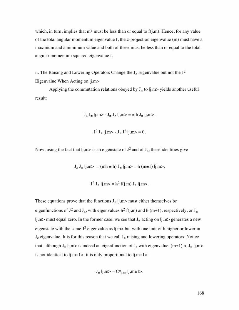
168

which, in turn, implies that m2 must be less than or equal to f(j,m). Hence, for any value

of the total angular momentum eigenvalue f, the z-projection eigenvalue (m) must have a

maximum and a minimum value and both of these must be less than or equal to the total

angular momentum squared eigenvalue f.

ii. The Raising and Lowering Operators Change the Jz Eigenvalue but not the J2

Eigenvalue When Acting on |j,m>

Applying the commutation relations obeyed by J± to |j,m> yields another useful

result:

Jz J± |j,m> - J± Jz |j,m> = ± h J± |j,m>,

J2 J± |j,m> - J± J2 |j,m> = 0.

Now, using the fact that |j,m> is an eigenstate of J2 and of Jz, these identities give

Jz J± |j,m> = (mh ± h) J± |j,m> = h (m±1) |j,m>,

J2 J± |j,m> = h2 f(j,m) J± |j,m>.

These equations prove that the functions J± |j,m> must either themselves be

eigenfunctions of J2 and Jz, with eigenvalues h2 f(j,m) and h (m+1), respectively, or J±

|j,m> must equal zero. In the former case, we see that J± acting on |j,m> generates a new

eigenstate with the same J2 eigenvalue as |j,m> but with one unit of h higher or lower in

Jz eigenvalue. It is for this reason that we call J± raising and lowering operators. Notice

that, although J± |j,m> is indeed an eigenfunction of Jz with eigenvalue (m±1) h, J± |j,m>

is not identical to |j,m±1>; it is only proportional to |j,m±1>:

J± |j,m> = C±j,m |j,m±1>.

169

Explicit expressions for these C±j,m coefficients will be obtained below. Notice also that

because the J± |j,m>, and hence |j,m±1>, have the same J2 eigenvalue as |j,m> (in fact,

sequential application of J± can be used to show that all |j,m'>, for all m', have this same

J2 eigenvalue), the J2 eigenvalue f(j,m) must be independent of m. For this reason, f can

be labeled by one quantum number j.

iii. The J2 Eigenvalues are Related to the Maximum and Minimum Jz Eigenvalues,

Which are Related to One Another

Earlier, we showed that there exists a maximum and a minimum value for m, for

any given total angular momentum. It is when one reaches these limiting cases that J±

|j,m> = 0 applies. In particular,

J+ |j,mmax> = 0,

J- |j,mmin> = 0.

Applying the following identities:

J- J+ = J2 - Jz2 -h Jz ,

J+ J- = J2 - Jz2 +h Jz,

respectively, to |j,mmax> and |j,mmin> gives

h2 { f(j,mmax) - mmax2 - mmax} = 0,

h2 { f(j,mmin) - mmin2 + mmin} = 0,

170

which immediately gives the J2 eigenvalue f(j,mmax) and f(j,mmin) in terms of mmax or

mmin:

f(j,mmax) = mmax (mmax+1),

f(j,mmin) = mmin (mmin-1).

So, we now know the J2 eigenvalues for |j,mmax> and |j,mmin>. However, we earlier

showed that |j,m> and |j,m-1> have the same J2 eigenvalue (when we treated the effect of

J± on |j,m>) and that the J2 eigenvalue is independent of m. If we therefore define the

quantum number j to be mmax , we see that the J2 eigenvalues are given by

J2 |j,m> = h2 j(j+1) |j,m>.

We also see that

f(j,m) = j(j+1) = mmax (mmax+1) = mmin (mmin-1),

from which it follows that

mmin = - mmax .

iv. The j Quantum Number Can Be Integer or Half-Integer

The fact that the m-values run from j to -j in unit steps (because of the property of

the J± operators), there clearly can be only integer or half-integer values for j. In the

former case, the m quantum number runs over -j, -j+1, -j+2, ..., -j+(j-1), 0, 1, 2, ... j;

in the latter, m runs over -j, -j+1, -j+2, ...-j+(j-1/2), 1/2, 3/2, ...j. Only integer and half-

integer values can range from j to -j in steps of unity. Species whose intrinsic angular

171

momenta are integers are known as Bosons and those with half-integer spin are called

Fermions.

v. More on J± |j,m>

Using the above results for the effect of J± acting on |j,m> and the fact that J+ and

J- are adjoints of one another (two operators F and G are adjoints if <ψ|F|χ> = <Gψ|χ>,

for all ψ and all χ) allows us to write:

<j,m| J- J+ |j,m> = <j,m| (J2 - Jz2 -h Jz ) |j,m>

= h2 {j(j+1)-m(m+1)} = <J+<j,m| J+|j,m> = (C+j,m)2,

where C+j,m is the proportionality constant between J+|j,m> and the normalized function

|j,m+1>. Likewise, the effect of J- can be expressed as

<j,m| J+ J- |j,m> = <j,m| (J2 - Jz2 +h Jz) |j,m>

= h2 {j(j+1)-m(m-1)} = <J-<j,m| J-|j,m> = (C-j,m)2,

where C-j,m is the proportionality constant between J- |j,m> and the normalized |j,m-1>.

Thus, we can solve for C±j,m after which the effect of J± on |j,m> is given by:

J± |j,m> = h {j(j+1) –m(m±1)}1/2 |j,m±1>.

2.7.3. Summary

The above results apply to any angular momentum operators. The essential

findings can be summarized as follows:

172

(i) J2 and Jz have complete sets of simultaneous eigenfunctions. We label these

eigenfunctions |j,m>; they are orthonormal in both their m- and j-type indices:

<j,m| j',m'> = δm,m' δj,j' .

(ii) These |j,m> eigenfunctions obey:

J2 |j,m> = h2 j(j+1) |j,m>, { j= integer or half-integer},

Jz |j,m> = h m |j,m>, { m = -j, in steps of 1 to +j}.

(iii) The raising and lowering operators J± act on |j,m> to yield functions that are

eigenfunctions of J2 with the same eigenvalue as |j,m> and eigenfunctions of Jz with

eigenvalue of (m±1) h :

J± |j,m> = h {j(j+1) - m(m±1)}1/2 |j,m±1>.

(iv) When J± acts on the extremal states |j,j> or |j,-j>, respectively, the result is zero.

The results given above are, as stated, general. Any and all angular momenta have

quantum mechanical operators that obey these equations. It is convention to designate

specific kinds of angular momenta by specific letters; however, it should be kept in mind

that no matter what letters are used, there are operators corresponding to J2, Jz, and J±

that obey relations as specified above, and there are eigenfunctions and eigenvalues that

have all of the properties obtained above. For electronic or collisional orbital angular

momenta, it is common to use L2 and Lz ; for electron spin, S2 and Sz are used; for

nuclear spin I2 and Iz are most common; and for molecular rotational angular momentum,

N2 and Nz are most common (although sometimes J2 and Jz may be used). Whenever two

or more angular momenta are combined or coupled to produce a total angular

momentum, the latter is designated by J2 and Jz.

173

2.7.4. Coupling of Angular Momenta

If the Hamiltonian under study contains terms that couple two or more angular

momenta J(i), then only the components of the total angular momentum J = Σi J(i) and

the total J2 will commute with H. It is therefore essential to label the quantum states of

the system by the eigenvalues of Jz and J2 and to construct variational trial or model

wave functions that are eigenfunctions of these total angular momentum operators. The

problem of angular momentum coupling has to do with how to combine eigenfunctions

of the uncoupled angular momentum operators, which are given as simple products of the

eigenfunctions of the individual angular momenta Πi |ji,mi>, to form eigenfunctions of J2

and Jz.

a. Eigenfunctions of Jz

Because the individual elements of J are formed additively, but J2 is not, it is

straightforward to form eigenstates of

Jz = Σi Jz(i);

simple products of the form Πi |ji,mi> are eigenfunctions of Jz:

Jz Πi |ji,mi> = Σk Jz(k) Πi |ji,mi> = Σk h mk Πi |ji,mi>,

and have Jz eigenvalues equal to the sum of the individual mk h eigenvalues. Hence, to

form an eigenfunction with specified J and M eigenvalues, one must combine only those

product states Πi |ji,mi> whose mih sum is equal to the specified M value.

b. Eigenfunctions of J2; the Clebsch-Gordon Series

174

The task is then reduced to forming eigenfunctions |J,M>, given particular values

for the {ji} quantum numbers. When coupling pairs of angular momenta { |j,m> and

|j',m'>}, the total angular momentum states can be written, according to what we

determined above, as

|J,M> = Σm,m' CJ,Mj,m;j',m' |j,m> |j',m'>,

where the coefficients CJ,Mj,m;j',m' are called vector coupling coefficients (because

angular momentum coupling is viewed much like adding two vectors j and j' to produce

another vector J), and where the sum over m and m' is restricted to those terms for which

m+m' = M. It is more common to express the vector coupling or so-called Clebsch-

Gordon (CG) coefficients as <j,m;j'm'|J,M> and to view them as elements of a matrix

whose columns are labeled by the coupled-state J,M quantum numbers and whose rows

are labeled by the quantum numbers characterizing the uncoupled product basis j,m;j',m'.

It turns out that this matrix can be shown to be unitary so that the CG coefficients obey:

Σm,m' <j,m;j'm'|J,M>* <j,m;j'm'|J',M'> = δJ,J' δM,M'

and

ΣJ,M <j,n;j'n'|J,M> <j,m;j'm'|J,M>* = δn,m δn',m'.

This unitarity of the CG coefficient matrix allows the inverse of the relation

giving coupled functions in terms of the product functions:

|J,M> = Σm,m' <j,m;j'm'|J,M> |j,m> |j',m'>

to be written as:

175

|j,m> |j',m'> = ΣJ,M <j,m;j'm'|J,M>* |J,M>

= ΣJ,M <J,M|j,m;j'm'> |J,M>.

This result expresses the product functions in terms of the coupled angular momentum

functions.

c. Generation of the CG Coefficients

The CG coefficients can be generated in a systematic manner; however, they can

also be looked up in books where they have been tabulated (e.g., see Table 2.4 of R. N.

Zare, Angular Momentum, John Wiley, New York (1988)). Here, we will demonstrate the

technique by which the CG coefficients can be obtained, but we will do so for rather

limited cases and refer the reader to more extensive tabulations for more cases.

The strategy we take is to generate the |J,J> state (i.e., the state with maximum M-

value) and to then use J- to generate |J,J-1>, after which the state |J-1,J-1> (i.e., the state

with one lower J-value) is constructed by finding a combination of the product states in

terms of which |J,J-1> is expressed (because both |J,J-1> and |J-1,J-1> have the same M-

value M=J-1) which is orthogonal to |J,J-1> (because |J-1,J-1> and |J,J-1> are

eigenfunctions of the Hermitian operator J2 corresponding to different eigenvalues, they

must be orthogonal). This same process is then used to generate |J,J-2> |J-1,J-2> and (by

orthogonality construction) |J-2,J-2>, and so on.

i. The States With Maximum and Minimum M-Values

We begin with the state |J,J> having the highest M-value. This state must be

formed by taking the highest m and the highest m' values (i.e., m=j and m'=j'), and is

given by:

|J,J> = |j,j> |j'j'>.

176

Only this one product is needed because only the one term with m=j and m'=j' contributes

to the sum in the above CG series. The state

|J,-J> = |j,-j> |j',-j'>

with the minimum M-value is also given as a single product state.

Notice that these states have M-values given as ±(j+j'); since this is the maximum M-

value, it must be that the J-value corresponding to this state is J= j+j'.

ii. States With One Lower M-Value But the Same J-Value

Applying J- to |J,J> , and expressing J- as the sum of lowering operators for the

two individual angular momenta:

J- = J-(1) + J-(2)

gives

J-|J,J> = h{J(J+1) -J(J-1)}1/2 |J,J-1>

= (J-(1) + J-(2)) |j,j> |j'j'>

= h{j(j+1) - j(j-1)}1/2 |j,j-1> |j',j'> + h{j'(j'+1)-j'(j'-1)}1/2 |j,j> |j',j'-1>.

This result expresses |J,J-1> as follows:

|J,J-1>= [{j(j+1)-j(j-1)}1/2 |j,j-1> |j',j'>

+ {j'(j'+1)-j'(j'-1)}1/2 |j,j> |j',j'-1>] {J(J+1) -J(J-1)}-1/2;

177

that is, the |J,J-1> state, which has M=J-1, is formed from the two product states |j,j-1>

|j',j'> and |j,j> |j',j'-1> that have this same M-value.

iii. States With One Lower J-Value

To find the state |J-1,J-1> that has the same M-value as the one found above but

one lower J-value, we must construct another combination of the two product states with

M=J-1 (i.e., |j,j-1> |j',j'> and |j,j> |j',j'-1>) that is orthogonal to the combination

representing |J,J-1>; after doing so, we must scale the resulting function so it is properly

normalized. In this case, the desired function is:

|J-1,J-1>= [{j(j+1)-j(j-1)}1/2 |j,j> |j',j'-1>

- {j'(j'+1)-j'(j'-1)}1/2 |j,j-1> |j',j'>] {J(J+1) -J(J-1)}-1/2 .

It is straightforward to show that this function is indeed orthogonal to |J,J-1>.

iv. States With Even One Lower J-Value

Having expressed |J,J-1> and |J-1,J-1> in terms of |j,j-1> |j',j'> and |j,j> |j',j'-1>,

we are now prepared to carry on with this stepwise process to generate the states |J,J-2>,

|J-1,J-2> and |J-2,J-2> as combinations of the product states with M=J-2. These product

states are |j,j-2> |j',j'>, |j,j> |j',j'-2>, and |j,j-1> |j',j'-1>. Notice that there are precisely as

many product states whose m+m' values add up to the desired M-value as there are total

angular momentum states that must be constructed (there are three of each in this case).

The steps needed to find the state |J-2,J-2> are analogous to those taken above:

a. One first applies J- to |J-1,J-1> and to |J,J-1> to obtain |J-1,J-2> and |J,J-2>,

respectively as combinations of |j,j-2> |j',j'>, |j,j> |j',j'-2>, and |j,j-1> |j',j'-1>.

b. One then constructs |J-2,J-2> as a linear combination of the |j,j-2> |j',j'>, |j,j> |j',j'-2>,

and |j,j-1> |j',j'-1> that is orthogonal to the combinations found for |J-1,J-2> and |J,J-2>.

Once |J-2,J-2> is obtained, it is then possible to move on to form |J,J-3>, |J-1,J-3>,

and |J-2,J-3> by applying J- to the three states obtained in the preceding application of the

process, and to then form |J-3,J-3> as the combination of |j,j-3> |j',j'>, |j,j> |j',j'-3>,

178

|j,j-2> |j',j'-1>, |j,j-1> |j',j'-2> that is orthogonal to the combinations obtained for |J,J-3>,

|J-1,J-3>, and |J-2,J-3>.

Again notice that there are precisely the correct number of product states (four

here) as there are total angular momentum states to be formed. In fact, the product states

and the total angular momentum states are equal in number and are both members of

orthonormal function sets (because J2(1), Jz(1), J2(2), and Jz(2) as well as J2 and Jz are

Hermitian operators which have complete sets of orthonormal eigenfunctions). This is

why the CG coefficient matrix is unitary; because it maps one set of orthonormal

functions to another, with both sets containing the same number of functions.

d. An Example

Let us consider an example in which the spin and orbital angular momenta of the

Si atom in its 3P ground state can be coupled to produce various 3PJ states. In this case,

the specific values for j and j' are j=S=1 and j'=L=1. We could, of course take j=L=1 and

j'=S=1, but the final wave functions obtained would span the same space as those we are

about to determine.

The state with highest M-value is the 3P(Ms=1, ML=1) state, which can be

represented by the product of an αα spin function (representing S=1, Ms=1) and a

3p13p0 spatial function (representing L=1, ML=1), where the first function corresponds to

the first open-shell orbital and the second function to the second open-shell orbital. Thus,

the maximum M-value is M= 2 and corresponds to a state with J=2:

|J=2,M=2> = |2,2> = αα 3p13p0 .

Clearly, the state |2,-2> would be given as ββ 3p-13p0.

The states |2,1> and |1,1> with one lower M-value are obtained by applying J- =

S- + L- to |2,2> as follows:

J- |2,2> = h{J(J+1)-M(M-1)}1/2 |2,1> = h{2(3)-2(1)}1/2 |2,1>

179

= (S- + L-) αα 3p13p0 .

To apply S- or L- to αα 3p13p0, one must realize that each of these operators is, in turn, a

sum of lowering operators for each of the two open-shell electrons:

S- = S-(1) + S-(2),

L- = L-(1) + L-(2).

The result above can therefore be continued as

(S- + L-) αα 3p13p0 = h{1/2(3/2)-1/2(-1/2)}1/2 βα 3p13p0

+ h{1/2(3/2)-1/2(-1/2)}1/2 αβ 3p13p0

+ h{1(2)-1(0)}1/2 αα 3p03p0

+ h{1(2)-0(-1)}1/2 αα 3p13p-1.

So, the function |2,1> is given by

|2,1> = [βα 3p13p0 + αβ 3p13p0 + {2}1/2 αα 3p03p0

+ {2}1/2 αα 3p13p-1]/2,

which can be rewritten as:

|2,1> = [(βα + αβ)3p13p0 + {2}1/2 αα (3p03p0 + 3p13p-1)]/2.

180

Writing the result in this way makes it clear that |2,1> is a combination of the product

states |S=1,MS=0> |L=1,ML=1> (the terms containing |S=1,MS=0> = 2-1/2(αβ+βα)) and

|S=1,MS=1> |L=1,ML=0> (the terms containing |S=1,MS=1> = αα).

There is a good chance that some readers have noticed that some of the terms in

the |2,1> function would violate the Pauli exclusion principle. In particular, the term αα

3p03p

0 places two electrons into the same orbitals and with the same spin. Indeed, this

electronic function would indeed violate the Pauli principle, and it should not be allowed

to contribute to the final Si 3PJ wave functions we are trying to form. The full resolution

of how to deal with this paradox is given in the following Subsection, but for now let me

say the following:

(i) Once you have learned that all of the spin-orbital product functions shown for |2,1>

(e.g., αα 3p03p

0 , (βα + αβ)3p13p0 , and αα 3p13p-1) represent Slater determinants (we

deal with this in the next Subsection) that are antisymmetric with respect to permutation

of any pair of electrons, you will understand that the Slater determinant corresponding to

αα 3p03p

0 vanishes.

(ii) If, instead of considering the 3s2 3p2 configuration of Si, we wanted to generate wave

functions for the 3s2 3p1 4p1 3PJ states of Si, the same analysis as shown above would

pertain, except that now the |2,1> state would have a contribution from αα 3p04p

0. This

contribution does not violate the Pauli principle, and its Slater determinant does not

vanish.

So, for the remainder of this treatment of the 3PJ states of Si, don’t worry about terms

arising that violate the Pauli principle; they will not contribute because their Slater

determinants will vanish.

To form the other function with M=1, the |1,1> state, we must find another

combination of |S=1,MS=0> |L=1,ML=1> and |S=1,MS=1> |L=1,ML=0> that is orthogonal

to |2,1> and is normalized. Since

|2,1> = 2-1/2 [|S=1,MS=0> |L=1,ML=1> + |S=1,MS=1> |L=1,ML=0>],

we immediately see that the requisite function is

181

|1,1> = 2-1/2 [|S=1,MS=0> |L=1,ML=1> - |S=1,MS=1> |L=1,ML=0>].

In the spin-orbital notation used above, this state is:

|1,1> = [(βα + αβ)3p13p0 - {2}1/2 αα (3p03p0 + 3p13p-1)]/2.

Thus far, we have found the 3PJ states with J=2, M=2; J=2, M=1; and J=1, M=1.

To find the 3PJ states with J=2, M=0; J=1, M=0; and J=0, M=0, we must once

again apply the J- tool. In particular, we apply J- to |2,1> to obtain |2,0> and we apply J-

to |1,1> to obtain |1,0>, each of which will be expressed in terms of |S=1,MS=0>

|L=1,ML=0>, |S=1,MS=1> |L=1,ML=-1>, and |S=1,MS=-1> |L=1,ML=1>. The |0,0>

state is then constructed to be a combination of these same product states which is

orthogonal to |2,0> and to |1,0>. The results are as follows:

|J=2,M=0> = 6-1/2[2 |1,0> |1,0> + |1,1> |1,-1> + |1,-1> |1,1>],

|J=1,M=0> = 2-1/2[|1,1> |1,-1> - |1,-1> |1,1>],

|J=0, M=0> = 3-1/2[|1,0> |1,0> - |1,1> |1,-1> - |1,-1> |1,1>],

where, in all cases, a short hand notation has been used in which the |S,MS> |L,ML>

product stated have been represented by their quantum numbers with the spin function

always appearing first in the product. To finally express all three of these new functions

in terms of spin-orbital products it is necessary to give the |S,MS> |L,ML> products with

M=0 in terms of these products. For the spin functions, we have:

|S=1,MS=1> = αα,

|S=1,MS=0> = 2-1/2(αβ+βα).

182

|S=1,MS=-1> = ββ.

For the orbital product function, we have:

|L=1, ML=1> = 3p13p0 ,

|L=1,ML=0> = 2-1/2(3p03p0 + 3p13p-1),

|L=1, ML=-1> = 3p03p-1.

e. Coupling Angular Momenta of Equivalent Electrons

If equivalent angular momenta are coupled (e.g., to couple the orbital angular

momenta of a p2 or d3 configuration), there is a tool one can use to determine which of

the term symbols violate the Pauli principle. To carry out this step, one forms all possible

unique (determinental) product states with non-negative ML and MS values and arranges

them into groups according to their ML and MS values. For example, the “boxes”

appropriate to the p2 orbital occupancy that we considered earlier for Si are shown below:

ML 2 1 0

---------------------------------------------------------

MS 1 |p1αp0α| |p1αp-1α|

0 |p1αp1β| |p1αp0β|, |p0αp1β| |p1αp-1β|,

|p-1αp1β|,

|p0αp0β|

There is no need to form the corresponding states with negative ML or negative MS

values because they are simply "mirror images" of those listed above. For example, the

state with ML= -1 and MS = -1 is |p-1βp0β|, which can be obtained from the ML = 1, MS

183

= 1 state |p1αp0α| by replacing α by β and replacing p1 by p-1.

Given the box entries, one can identify those term symbols that arise by applying

the following procedure over and over until all entries have been accounted for:

i. One identifies the highest MS value (this gives a value of the total spin quantum

number that arises, S) in the box. For the above example, the answer is S = 1.

ii. For all product states of this MS value, one identifies the highest ML value (this gives a

value of the total orbital angular momentum, L, that can arise for this S). For the above

example, the highest ML within the MS =1 states is ML = 1 (not ML = 2), hence L=1.

iii. Knowing an S, L combination, one knows the first term symbol that arises from this

configuration. In the p2 example, this is 3P.

iv. Because the level with this L and S quantum numbers contains (2L+1)(2S+1) states

with ML and MS quantum numbers running from -L to L and from -S to S, respectively,

one must remove from the original box this number of product states. To do so, one

simply erases from the box one entry with each such ML and MS value. Actually, since

the box need only show those entries with non-negative ML and MS values, only these

entries need be explicitly deleted. In the 3P example, this amounts to deleting nine

product states with ML, MS values of 1,1; 1,0; 1,-1; 0,1; 0,0; 0,-1; -1,1; -1,0; -1,-1.

v. After deleting these entries, one returns to step 1 and carries out the process again. For

the p2 example, the box after deleting the first nine product states looks as follows (those

that appear in italics should be viewed as already deleted in counting all of the 3P states):

ML 2 1 0

---------------------------------------------------------

MS 1 |p1αp0α| |p1αp-1α|

0 |p1αp1β| |p1αp0β|, |p0αp1β| |p1αp-1β|,

|p-1αp1β|,

|p0αp0β|

It should be emphasized that the process of deleting or crossing off entries in various ML,

184

MS boxes involves only counting how many states there are; by no means do we identify

the particular L,S,ML,MS wave functions when we cross out any particular entry in a box.

For example, when the |p1αp0β| product is deleted from the ML= 1, MS=0 box in

accounting for the states in the 3P level, we do not claim that |p1αp0β| itself is a member

of the 3P level; the |p0αp1β| product state could just as well been eliminated when

accounting for the 3P states.

Returning to the p2 example at hand, after the 3P term symbol's states have been

accounted for, the highest MS value is 0 (hence there is an S=0 state), and within this MS

value, the highest ML value is 2 (hence there is an L=2 state). This means there is a 1D

level with five states having ML = 2,1,0,-1,-2. Deleting five appropriate entries from the

above box (again denoting deletions by italics) leaves the following box:

ML 2 1 0

---------------------------------------------------------

MS 1 |p1αp0α| |p1αp-1α|

0 |p1αp1β| |p1αp0β|, |p0αp1β| |p1αp-1β|,

|p-1αp1β|,

|p0αp0β|

The only remaining entry, which thus has the highest MS and ML values, has MS = 0 and

ML = 0. Thus there is also a 1S level in the p2 configuration.

Thus, unlike the non-equivalent 3p14p1 case, in which 3P, 1P, 3D, 1D, 3S, and 1S

levels arise, only the 3P, 1D, and 1S arise in the p2 situation. This "box method" is useful

to carry out whenever one is dealing with equivalent angular momenta.

If one has mixed equivalent and non-equivalent angular momenta, one can

determine all possible couplings of the equivalent angular momenta using this method

and then use the simpler vector coupling method to add the non-equivalent angular

185

momenta to each of these coupled angular momenta. For example, the p2d1 configuration

can be handled by vector coupling (using the straightforward non-equivalent procedure)

L=2 (the d orbital) and S=1/2 (the third electron's spin) to each of 3P, 1D, and 1S arising

from the p2 configuration. The result is 4F, 4D, 4P, 2F, 2D, 2P, 2G, 2F, 2D, 2P, 2S, and 2D.

2.8. Rotations of Molecules

2.8.1. Rotational Motion For Rigid Diatomic and Linear Polyatomic Molecules

This Schrödinger equation relates to the rotation of diatomic and linear

polyatomic molecules. It also arises when treating the angular motions of electrons in

any spherically symmetric potential.

A diatomic molecule with fixed bond length R rotating in the absence of any

external potential is described by the following Schrödinger equation:

- h2/2µ {(R2sinθ)-1∂/∂θ (sinθ ∂/∂θ) + (R2sin2θ)-1 ∂2/∂φ2 } ψ = E ψ

or

L2ψ/2µR2 = E ψ,

where L2 is the square of the total angular momentum operator Lx2 + Ly

2 + Lz2 expressed

in polar coordinates above. The angles θ and φ describe the orientation of the diatomic

molecule's axis relative to a laboratory-fixed coordinate system, and µ is the reduced

mass of the diatomic molecule µ=m1m2/(m1+m2). The differential operators can be seen

to be exactly the same as those that arose in the hydrogen-like-atom case discussed earlier

in this Chapter. Therefore, the same spherical harmonics that served as the angular parts

of the wave function in the hydrogen-atom case now serve as the entire wave function for

the so-called rigid rotor: ψ = YJ,M(θ,φ). These are exactly the same functions as we

186

plotted earlier when we graphed the s (L=0), p (L=1), and d (L=2) orbitals. The energy

eigenvalues corresponding to each such eigenfunction are given as:

EJ = h2 J(J+1)/(2µR2) = B J(J+1)

and are independent of M. Thus each energy level is labeled by J and is 2J+1-fold

degenerate (because M ranges from -J to J). Again, this is just like we saw when we

looked at the hydrogen orbitals; the p orbitals are 3-fold degenerate and the d orbitals are

5-fold degenerate. The so-called rotational constant B (defined as h2/2µR2) depends on

the molecule's bond length and reduced mass. Spacings between successive rotational

levels (which are of spectroscopic relevance because, as shown in Chapter 6, angular

momentum selection rules often restrict the changes ΔJ in J that can occur upon photon

absorption to 1,0, and -1) are given by

ΔE = B (J+1)(J+2) - B J(J+1) = 2B(J+1).

These energy spacings are of relevance to microwave spectroscopy which probes the

rotational energy levels of molecules. In fact, microwave spectroscopy offers the most

direct way to determine molecular rotational constants and hence molecular bond lengths.

The rigid rotor provides the most commonly employed approximation to the

rotational energies and wave functions of linear molecules. As presented above, the

model restricts the bond length to be fixed. Vibrational motion of the molecule gives rise

to changes in R, which are then reflected in changes in the rotational energy levels (i.e.,

there are different B values for different vibrational levels). The coupling between

rotational and vibrational motion gives rise to rotational B constants that depend on

vibrational state as well as dynamical couplings, called centrifugal distortions, which

cause the total ro-vibrational energy of the molecule to depend on rotational and

vibrational quantum numbers in a non-separable manner.

Within this rigid rotor model, the absorption spectrum of a rigid diatomic

molecule should display a series of peaks, each of which corresponds to a specific J → J

+ 1 transition. The energies at which these peaks occur should grow linearly with J as

187

shown above. An example of such a progression of rotational lines is shown in the Fig.

2.23.

Figure 2.23. Typical rotational absorption profile showing intensity vs. J value of the

absorbing level

The energies at which the rotational transitions occur appear to fit the ΔE = 2B (J+1)

formula rather well. The intensities of transitions from level J to level J+1 vary strongly

with J primarily because the population of molecules in the absorbing level varies with J.

These populations PJ are given, when the system is at equilibrium at temperature T, in

terms of the degeneracy (2J+1) of the Jth level and the energy of this level B J(J+1) by the

Boltzmann formula:

PJ = Q-1 (2J+1) exp(-BJ(J+1)/kT),

where Q is the rotational partition function:

Q = ΣJ (2J+1) exp(-BJ(J+1)/kT).

For low values of J, the degeneracy is low and the exp(-BJ(J+1)/kT) factor is near unity.

As J increases, the degeneracy grows linearly but the exp(-BJ(J+1)/kT) factor decreases

188

more rapidly. As a result, there is a value of J, given by taking the derivative of (2J+1)

exp(-BJ(J+1)/kT) with respect to J and setting it equal to zero,

2Jmax + 1 = 2kT/B

at which the intensity of the rotational transition is expected to reach its maximum. This

behavior is clearly displayed in the above figure.

The eigenfunctions belonging to these energy levels are the spherical harmonics

YL,M(θ,φ) which are normalized according to

€

(Y *L ,M (θ,φ)YL ',M '0

2π

∫ (θ,φ)sinθdφdθ0

π

∫ = δL,L' δM,M' .

As noted above, these functions are identical to those that appear in the solution of the

angular part of Hydrogenic atoms. The above energy levels and eigenfunctions also apply

to the rotation of rigid linear polyatomic molecules; the only difference is that the

moment of inertia I entering into the rotational energy expression, which is µR2 for a

diatomic, is given by

I = Σa ma Ra2

where ma is the mass of the ath atom and Ra is its distance from the center of mass of the

molecule to this atom.

2.8.2. Rotational Motions of Rigid Non-Linear Molecules

a. The Rotational Kinetic Energy

The classical rotational kinetic energy for a rigid polyatomic molecule is

Hrot = Ja2/2Ia + Jb2/2Ib + Jc2/2Ic

189

where the Ik (k = a, b, c) are the three principal moments of inertia of the molecule (the

eigenvalues of the moment of inertia tensor). This tensor has elements in a Cartesian

coordinate system (K, K' = X, Y, Z), whose origin is located at the center of mass of the

molecule, that can be computed as:

IK,K = Σj mj (Rj2 - R2K,j) (for K = K')

IK,K' = - Σj mj RK,j RK',j (for K ≠ K').

As discussed in more detail in R. N. Zare, Angular Momentum, John Wiley, New York

(1988), the components of the corresponding quantum mechanical angular momentum

operators along the three principal axes are:

Ja = -ih cosχ [cotθ ∂/∂χ - (sinθ)-1∂/∂φ ] - -ih sinχ ∂/∂θ

Jb = ih sinχ [cotθ ∂/∂χ - (sinθ)-1∂/∂φ ] - -ih cosχ ∂/∂θ

Jc = - ih ∂/∂χ.

The angles θ, φ, and χ are the Euler angles needed to specify the orientation of the rigid

molecule relative to a laboratory-fixed coordinate system. The corresponding square of

the total angular momentum operator J2 can be obtained as

J2 = Ja2 + Jb2 + Jc2

= - h2 ∂2/∂θ2 - h2cotθ ∂/∂θ

+ h2 (1/sin2θ) (∂2/∂φ2 + ∂2/∂χ2 - 2 cosθ∂2/∂φ∂χ),

190

and the component along the lab-fixed Z axis JZ is - ih ∂/∂φ as we saw much earlier in

this text.

b. The Eigenfunctions and Eigenvalues for Special Cases

i. Spherical Tops

When the three principal moment of inertia values are identical, the molecule is

termed a spherical top. In this case, the total rotational energy can be expressed in terms

of the total angular momentum operator J2

Hrot = J2/2I.

As a result, the eigenfunctions of Hrot are those of J2 and Ja as well as JZ both of which

commute with J2 and with one another. JZ is the component of J along the lab-fixed Z-

axis and commutes with Ja because JZ = - ih ∂/∂φ and Ja = - ih ∂/∂χ act on different

angles. The energies associated with such eigenfunctions are

E(J,K,M) = h2 J(J+1)/2I2,

for all K (i.e., Ja quantum numbers) ranging from -J to J in unit steps and for all M (i.e.,

JZ quantum numbers) ranging from -J to J. Each energy level is therefore (2J + 1)2

degenerate because there are 2J + 1 possible K values and 2J + 1 possible M values for

each J.

The eigenfunctions |J,M,K> of J2, JZ and Ja , are given in terms of the set of so-

called rotation matrices DJ,M,K:

|J,M,K> = 2J + 18 π2 D*J,M,K(θ,φ,χ)

which obey

191

J2 |J,M,K> = h2 J(J+1) |J,M,K>,

Ja |J,M,K> = h K |J,M,K>,

JZ |J,M,K> = h M |J,M,K>.

These DJ,M,K functions are proportional to the spherical harmonics YJ,M(θ,φ) multiplied by

exp(iKχ), which reflects its χ-dependence.

ii. Symmetric Tops

Molecules for which two of the three principal moments of inertia are equal are

called symmetric tops. Those for which the unique moment of inertia is smaller than the

other two are termed prolate symmetric tops; if the unique moment of inertia is larger

than the others, the molecule is an oblate symmetric top. An American football is prolate,

and a Frisbee is oblate.

Again, the rotational kinetic energy, which is the full rotational Hamiltonian, can

be written in terms of the total rotational angular momentum operator J2 and the

component of angular momentum along the axis with the unique principal moment of

inertia:

Hrot = J2/2I + Ja2{1/2Ia - 1/2I}, for prolate tops

Hrot = J2/2I + Jc2{1/2Ic - 1/2I}, for oblate tops.

Here, the moment of inertia I denotes that moment that is common to two directions; that

is, I is the non-unique moment of inertia. As a result, the eigenfunctions of Hrot are those

of J2 and Ja or Jc (and of JZ), and the corresponding energy levels are:

E(J,K,M) = h2 J(J+1)/2I2 + h2 K2 {1/2Ia - 1/2I},

192

for prolate tops

E(J,K,M) = h2 J(J+1)/2I2 + h2 K2 {1/2Ic - 1/2I},

for oblate tops, again for K and M (i.e., Ja or Jc and JZ quantum numbers, respectively)

ranging from -J to J in unit steps. Since the energy now depends on K, these levels are

only 2J + 1 degenerate due to the 2J + 1 different M values that arise for each J value.

Notice that for prolate tops, because Ia is smaller than I, the energies increase with

increasing K for given J. In contrast, for oblate tops, since Ic is larger than I, the energies

decrease with K for given J. The eigenfunctions |J, M,K> are the same rotation matrix

functions as arise for the spherical-top case, so they do not require any further discussion

at this time.

iii. Asymmetric Tops

The rotational eigenfunctions and energy levels of a molecule for which all three

principal moments of inertia are distinct (a so-called asymmetric top) cannot analytically

be expressed in terms of the angular momentum eigenstates and the J, M, and K quantum

numbers. In fact, no one has ever solved the corresponding Schrödinger equation for this

case. However, given the three principal moments of inertia Ia, Ib, and Ic, a matrix

representation of each of the three contributions to the rotational Hamiltonian

Hrot = Ja2/2Ia + Jb2/2Ib + Jc2/2Ic

can be formed within a basis set of the {|J, M, K>} rotation-matrix functions discussed

earlier. This matrix will not be diagonal because the |J, M, K> functions are not

eigenfunctions of the asymmetric top Hrot. However, the matrix can be formed in this

basis and subsequently brought to diagonal form by finding its eigenvectors {Cn, J,M,K}

and its eigenvalues {En}. The vector coefficients express the asymmetric top eigenstates

as

193

ψn (θ, φ, χ) = ΣJ, M, K Cn, J,M,K |J, M, K>.

Because the total angular momentum J2 still commutes with Hrot, each such eigenstate

will contain only one J-value, and hence ψn can also be labeled by a J quantum number:

ψn,J (θ, φ, χ) = Σ M, K Cn, J,M,K |J, M, K>.

To form the only non-zero matrix elements of Hrot within the |J, M, K> basis, one

can use the following properties of the rotation-matrix functions (see, for example, R. N.

Zare, Angular Momentum, John Wiley, New York (1988)):

<J, M, K| Ja2| J, M, K> = <J, M, K| Jb 2| J, M, K>

= 1/2 <J, M, K| J2 - Jc2 | J, M, K> = h2 [ J(J+1) - K2 ],

<J, M, K| Jc2| J, M, K> = h2 K2,

<J, M, K| Ja2| J, M, K ± 2> = - <J, M, K| Jb 2| J, M, K ± 2>

= h2 [J(J+1) - K(K± 1)]1/2 [J(J+1) -(K± 1)(K± 2)]1/2

<J, M, K| Jc2| J, M, K ± 2> = 0.

Each of the elements of Jc2, Ja2, and Jb2 must, of course, be multiplied, respectively, by

1/2Ic, 1/2Ia, and 1/2Ib and summed together to form the matrix representation of Hrot.

The diagonalization of this matrix then provides the asymmetric top energies and wave

functions.

194

2.9. Vibrations of Molecules

This Schrödinger equation forms the basis for our thinking about bond stretching and

angle bending vibrations as well as collective vibrations in solids called phonons.

The radial motion of a diatomic molecule in its lowest (J=0) rotational level can

be described by the following Schrödinger equation:

- (h2/2µ) r-2∂/∂r (r2∂/∂r) ψ +V(r) ψ = E ψ,

where µ is the reduced mass µ = m1m2/(m1+m2) of the two atoms. If the molecule is

rotating, then the above Schrödinger equation has an additional term J(J+1) h2/2µ r-2 ψ

on its left-hand side. Thus, each rotational state (labeled by the rotational quantum

number J) has its own vibrational Schrödinger equation and thus its own set of vibrational

energy levels and wave functions. It is common to examine the J=0 vibrational problem

and then to use the vibrational levels of this state as approximations to the vibrational

levels of states with non-zero J values (treating the vibration-rotation coupling via

perturbation theory). Let us thus focus on the J=0 situation.

By substituting ψ= F(r)/r into this equation, one obtains an equation for F(r) in

which the differential operators appear to be less complicated:

- h2/2µ d2F/dr2 + V(r) F = E F.

This equation is exactly the same as the equation seen earlier in this text for the radial

motion of the electron in the hydrogen-like atoms except that the reduced mass µ replaces

the electron mass m and the potential V(r) is not the Coulomb potential.

If the vibrational potential is approximated as a quadratic function of the bond

displacement x = r-re expanded about the equilibrium bond length re where V has its

minimum:

195

V = 1/2 k(r-re)2,

the resulting harmonic-oscillator equation can be solved exactly. Because the potential V

grows without bound as x approaches ∞ or -∞, only bound-state solutions exist for this

model problem. That is, the motion is confined by the nature of the potential, so no

continuum states exist in which the two atoms bound together by the potential are

dissociated into two separate atoms.

In solving the radial differential equation for this potential, the large-r behavior is

first examined. For large-r, the equation reads:

d2F/dx2 = 1/2 k x2 (2µ/h2) F = (kµ/h2) x2 F,

where x = r-re is the bond displacement away from equilibrium. Defining β2 =(kµ/h2) and

ξ= β 1/2 x as a new scaled radial coordinate, and realizing that

d2/dx2 = β d2/dξ2

allows the large-r Schrödinger equation to be written as:

d2F/dξ2 = ξ2 F

which has the solution

Flarge-r = exp(- ξ2/2).

The general solution to the radial equation is then expressed as this large-r

solution multiplied by a power series in the ζ variable:

F = exp(- ξ2/2)

€

ξ nCnn= 0∑ ,

196

where the Cn are coefficients to be determined. Substituting this expression into the full

radial equation generates a set of recursion equations for the Cn amplitudes. As in the

solution of the hydrogen-like radial equation, the series described by these coefficients is

divergent unless the energy E happens to equal specific values. It is this requirement that

the wave function not diverge so it can be normalized that yields energy quantization.

The energies of the states that arise by imposing this non-divergence condition are given

by:

En = h (k/µ)1/2 (n+1/2),

and the eigenfunctions are given in terms of the so-called Hermite polynomials Hn(y) as

follows:

ψn(x) = (n! 2n)-1/2 (β/π)1/4 exp(- βx2/2) Hn(β1/2 x),

where β =(kµ/h2)1/2. Within this harmonic approximation to the potential, the vibrational

energy levels are evenly spaced:

ΔE = En+1 - En = h (k/µ)1/2 .

In experimental data such evenly spaced energy level patterns are seldom seen; most

commonly, one finds spacings En+1 - En that decrease as the quantum number n

increases. In such cases, one says that the progression of vibrational levels displays

anharmonicity.

Because the Hermite functions Hn are odd or even functions of x (depending on

whether n is odd or even), the wave functions ψn(x) are odd or even. This splitting of the

solutions into two distinct classes is an example of the effect of symmetry; in this case,

the symmetry is caused by the symmetry of the harmonic potential with respect to

reflection through the origin along the x-axis (i.e., changing x to –x). Throughout this

text, many symmetries arise; in each case, symmetry properties of the potential cause the

solutions of the Schrödinger equation to be decomposed into various symmetry

197

groupings. Such symmetry decompositions are of great use because they provide

additional quantum numbers (i.e., symmetry labels) by which the wave functions and

energies can be labeled.

The basic idea underlying how such symmetries split the solutions of the

Schrödinger equation into different classes relates to the fact that a symmetry operator

(e.g., the reflection plane in the above example) commutes with the Hamiltonian. That is,

the symmetry operator S obeys

S H = H S.

So S leaves H unchanged as it acts on H (this allows us to pass S through H in the above

equation). Any operator that leaves the Hamiltonian (i.e., the energy) unchanged is called

a symmetry operator.

If you have never learned about how point group symmetry can be used to help

simplify the solution of the Schrödinger equation, this would be a good time to interrupt

your reading and go to Chapter 4 and read the material there.

The harmonic oscillator energies and wave functions comprise the simplest

reasonable model for vibrational motion. Vibrations of a polyatomic molecule are often

characterized in terms of individual bond-stretching and angle-bending motions, each of

which is, in turn, approximated harmonically. This results in a total vibrational wave

function that is written as a product of functions, one for each of the vibrational

coordinates.

Two of the most severe limitations of the harmonic oscillator model, the lack of

anharmonicity (i.e., non-uniform energy level spacings) and lack of bond dissociation,

result from the quadratic nature of its potential. By introducing model potentials that

allow for proper bond dissociation (i.e., that do not increase without bound as x → ∞),

the major shortcomings of the harmonic oscillator picture can be overcome. The so-called

Morse potential (see Fig. 2.24)

V(r) = De (1-exp(-a(r-re)))2,

198

is often used in this regard. In this form, the potential is zero at r = re, the equilibrium

bond length and is equal to De as r →∞. Sometimes, the potential is written as

V(r) = De (1-exp(-a(r-re)))2 -De

so it vanishes as r →∞ and is equal to –De at r = re. The latter form is reflected in Fig.

2.24.

Figure 2.24. Morse potential energy as a function of bond length

In the Morse potential function, De is the bond dissociation energy, re is the equilibrium

bond length, and a is a constant that characterizes the steepness of the potential and thus

affects the vibrational frequencies. The advantage of using the Morse potential to

improve upon harmonic-oscillator-level predictions is that its energy levels and wave

functions are also known exactly. The energies are given in terms of the parameters of the

potential as follows:

En = h(k/µ)1/2 { (n+1/2) - (n+1/2)2 h(k/µ)1/2/4De },

199

where the force constant is given in terms of the Morse potential’s parameters by k=2De

a2. The Morse potential supports both bound states (those lying below the dissociation

threshold for which vibration is confined by an outer turning point) and continuum states

lying above the dissociation threshold (for which there is no outer turning point and thus

the no spatial confinement). Its degree of anharmonicity is governed by the ratio of the

harmonic energy h(k/µ)1/2 to the dissociation energy De.

The energy spacing between vibrational levels n and n+1 are given by

En+1 – En = h(k/µ)1/2 { 1 - (n+1) h(k/µ)1/2/2De }.

These spacings decrease until n reaches the value nmax at which

{ 1 - (nmax+1) h(k/µ)1/2/2De } = 0,

after which the series of bound Morse levels ceases to exist (i.e., the Morse potential has

only a finite number of bound states) and the Morse energy level expression shown above

should no longer be used. It is also useful to note that, if [2Deµ]1/2/[a h] becomes too small

(i.e., < 1.0 in the Morse model), the potential may not be deep enough to support any

bound levels. It is true that some attractive potentials do not have a large enough De value

to have any bound states, and this is important to keep in mind. So, bound states are to be

expected when there is a potential well (and thus the possibility of inner- and outer-

turning points for the classical motion within this well) but only if this well is deep

enough.

The eigenfunctions of the harmonic and Morse potentials display nodal character

analogous to what we have seen earlier in the particle-in-boxes model problems. Namely,

as the energy of the vibrational state increases, the number of nodes in the vibrational

wave function also increases. The state having vibrational quantum number v has v

nodes. I hope that by now the student is getting used to seeing the number of nodes

increase as the quantum number and hence the energy grows. As the quantum number v

200

grows, not only does the wave function have more nodes, but its probability distribution

becomes more and more like the classical spatial probability, as expected. In particular

for large-v, the quantum and classical probabilities are similar and are large near the outer

turning point where the classical velocity is low. They also have large amplitudes near

the inner turning point, but this amplitude is rather narrow because the Morse potential

drops off strongly to the right of this turning point; in contrast, to the left of the outer

turning point, the potential decreases more slowly, so the large amplitudes persist over

longer ranges near this turning point.

2.10 Chapter Summary

In this Chapter, you should have learned about the following things:

1. Free particle energies and wave functions and their densities of states, as applied to

polyenes, electron in surfaces, solids, and nanoscopic materials and as applied to bands of

orbitals in solids.

2. The tight-binding or Hückel model for chemical bonding.

3. The hydrogenic radial and angular wave functions. These same angular functions occur

whenever one is dealing with a potential that depends only on the radial coordinate, not

the angular coordinates.

4. Electron tunneling and quasi-bound resonance states.

5. Angular momentum including coupling two or more angular momenta, and angular

momentum as applied to rotations of rigid molecules including rigid rotors, symmetric,

spherical, and asymmetric top rotations. Why half-integral angular momenta cannot be

thought of as arising from rotational motion of a physical body.

6. Vibrations of diatomic molecules including the harmonic oscillator and Morse

oscillator models including harmonic frequencies and anharmonicity.