7

Chapter 2 Introduction to Physics of Charging and

Discharging

The fundamental physical concepts that account for space charging are described in this chapter. The appendices describe this further with equations and examples.

2.1 Physical Concepts Spacecraft charging occurs when charged particles from the surrounding plasma and energetic particle environment stop on the spacecraft, either on the surface, on interior parts, in dielectrics, or in conductors. Other items affecting charging include biased solar arrays or plasma emitters. Charging can also occur when photoemission occurs; that is, solar photons cause surfaces to emit photoelectrons. Events after that determine whether the charging causes problems or not.

2.1.1 Plasma A plasma is a partially ionized gas in which some of the atoms and molecules that make up the gas have some or all of their electrons stripped off leaving a mixture of ions and electrons that can develop a sheath that can extend over several Debye lengths. Except for LEO where ionized oxygen (O+) is the most abundant species, the simplest ion, a proton (corresponding to ionized hydrogen, H+) is generally the most abundant ion in the environments considered here. The energy of the plasma, its electrons and ions, is often described in units of electron volts (eV). This is the kinetic energy that is given to the electron or ion if it is accelerated by an electric potential of that many volts. While temperature (T) is generally used to describe the disordered

8 Chapter 2

microscopic motion of a group of particles, plasma physicists also use it as another unit of measure to describe the kinetic energy of the plasma. For electrons, numerically T(K) equals T(eV) × 11,604; that is, 4,300 eV is equivalent to 50 million kelvins (K).

The kinetic energy of a particle is given by the following equation:

E =12

mv 2

(2.1-1)

where:

E = energy

m = mass of the particle

v = velocity of the particle.

Because of the difference in mass (~1:1836 for electrons to protons), electrons in a plasma in thermal equilibrium generally have a velocity ~43 times that of protons. This translates into a net instantaneous flux or current of electrons onto a spacecraft that is much higher than that of the ions (typically nanoamperes per square centimeter, nA/cm2, for electrons versus picoamperes per square centimeter, pA/cm2, for protons at geosynchronous orbit). This difference in flux is one reason for the observed charging effects (a surplus of negative charges on affected regions). For electrons, numerically the velocity (ve) equals sqrt(E) × 593 kilometers per second (km/s) and for protons the velocity (vp) equals sqrt(E) × 13.8 km/s, when E is in eV.

Although a plasma may be described by its average energy, there is actually a distribution of energies. The rate of charging in the interior of the spacecraft is a function of the flux versus energy, or spectrum, of the plasma at energies well in excess of the mean plasma energies (for GEO, the plasma mean energy may reach a few tens of kilo-electron volts, keV). Surface charging is usually correlated with electrons in the 0 to ~50 keV energy range, while significant internal charging is associated with the high-energy electrons (100 keV to 3 mega-electron volts, MeV).

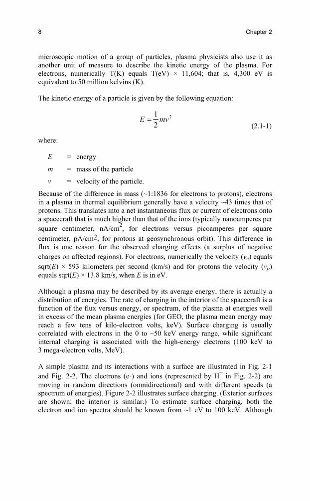
A simple plasma and its interactions with a surface are illustrated in Fig. 2-1 and Fig. 2-2. The electrons (e-) and ions (represented by H+ in Fig. 2-2) are moving in random directions (omnidirectional) and with different speeds (a spectrum of energies). Figure 2-2 illustrates surface charging. (Exterior surfaces are shown; the interior is similar.) To estimate surface charging, both the electron and ion spectra should be known from ~1 eV to 100 keV. Although

Introduction to Physics of Charging and Discharging 9

fluxes might be directed, omnidirectional fluxes are assumed in this document because spacecraft orientation relative to the plasma is often not well-defined.

Fig. 2-1. Illustration of a simple plasma.

Fig. 2-2. Plasma interactions with spacecraft surfaces.

e -

e -

e -

e - e -

e - e -

e -

e -

H +

H +

H +

H +

H +

H +

H +

H +

H +

10 Chapter 2

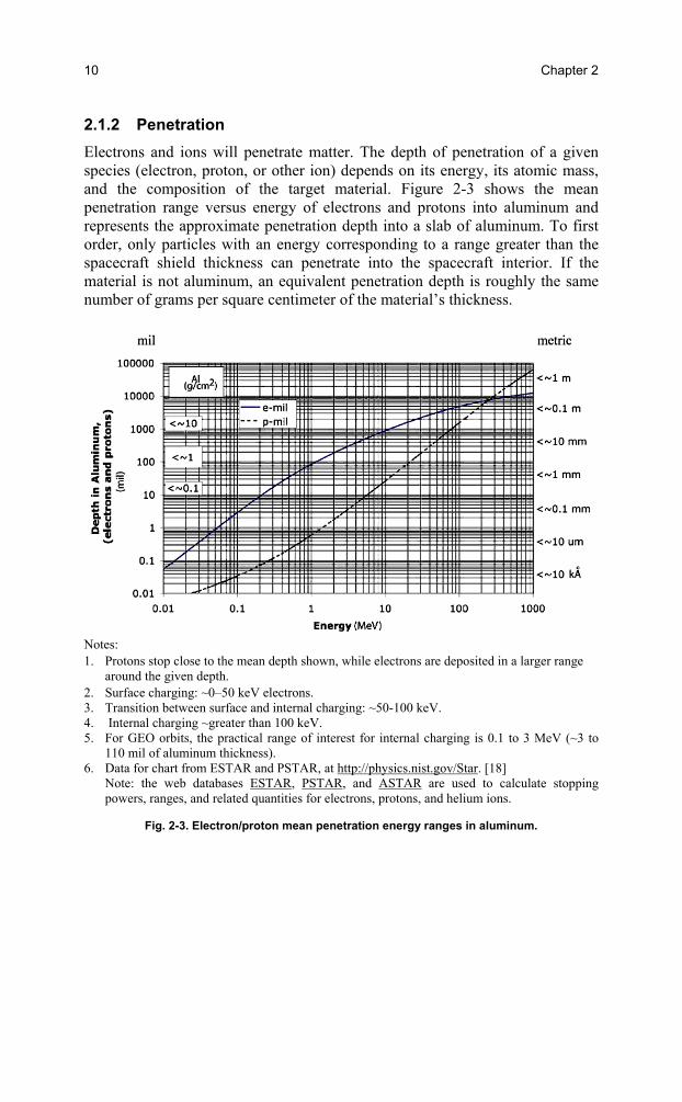
2.1.2 Penetration Electrons and ions will penetrate matter. The depth of penetration of a given species (electron, proton, or other ion) depends on its energy, its atomic mass, and the composition of the target material. Figure 2-3 shows the mean penetration range versus energy of electrons and protons into aluminum and represents the approximate penetration depth into a slab of aluminum. To first order, only particles with an energy corresponding to a range greater than the spacecraft shield thickness can penetrate into the spacecraft interior. If the material is not aluminum, an equivalent penetration depth is roughly the same number of grams per square centimeter of the material’s thickness.

Notes: 1. Protons stop close to the mean depth shown, while electrons are deposited in a larger range

around the given depth. 2. Surface charging: ~0–50 keV electrons. 3. Transition between surface and internal charging: ~50-100 keV. 4. Internal charging ~greater than 100 keV. 5. For GEO orbits, the practical range of interest for internal charging is 0.1 to 3 MeV (~3 to

110 mil of aluminum thickness). 6. Data for chart from ESTAR and PSTAR, at http://physics.nist.gov/Star. [18] Note: the web databases ESTAR, PSTAR, and ASTAR are used to calculate stopping

powers, ranges, and related quantities for electrons, protons, and helium ions.

Fig. 2-3. Electron/proton mean penetration energy ranges in aluminum.

Introduction to Physics of Charging and Discharging 11

This document uses the terms surface charging and internal charging. The literature also uses the terms buried dielectric charge or deep dielectric charge for internal charging. These terms are misleading because they give the impression that only dielectrics can accumulate charge. Although dielectrics can accumulate charge and discharge to cause damage, ungrounded conductors can also accumulate charge and must also be considered an internal charging threat. In fact, ungrounded conductors can discharge with a higher peak current and a higher rate of change of current than a dielectric and can be a greater threat.

Based on typical spacecraft construction, there is usually an interior section that is referred to in this document as internal. It is assumed that this interior section has shielding of at least 3 mil of aluminum equivalent, corresponding to electron energies greater than 0.1 MeV. Surface charging would be the outer layers of the spacecraft corresponding to 2 mil of aluminum or 0 to 50 keV electrons. Obviously, the surface/internal charging cutoff depends on spacecraft construction. Protons are often not considered for spacecraft charging because the greater impinging flux of electrons at the same energy and (for internal charging) the lesser penetration of protons reduces the internal flux to a negligible amount. Higher atomic mass particles are even less of a threat because of their much lower fluxes.

Because electrons may stop at a depth less than their maximum penetration depth and because the electron spectrum is continuous, the penetration-depth/charging-region will be continuous, ranging from the charges deposited on the exterior surface to those deposited deep in the interior. Internal charging as used here often is equivalent to “inside the Faraday cage.” For a spacecraft that is built with a Faraday cage thickness of 30 or more mil of aluminum equivalent, this would mean that internal effects deal with the portion of the electron spectrum above 500 keV and the proton spectrum above 10 MeV. At GEO orbits, the practical range of energy for internal charging is 100 keV to about 3 MeV, bounded on the lower end by the fact that most spacecraft have at least 3 mil of shielding and on the upper end by the fact that, as will be shown later, common GEO environments above 3 MeV do not have enough plasma flux to cause internal charging problems.

Figure 2-4 illustrates the concept that energetic electrons will penetrate into interior portions of a spacecraft. Having penetrated, the electrons may be stopped in dielectrics or on ungrounded conductors. If too many electrons accumulate, the resultant high electric fields inside the spacecraft may cause an ESD to a nearby victim circuit.

12 Chapter 2

Fig. 2-4. Internal charging, illustrated.

Note that the internal charging resembles surface charging with the exception that circuits are rarely exposed victims on the exterior surface of a spacecraft, and thus (with the condition that charging rates are slower) internal charging results in a greater direct threat to circuits.

The term “ESD” in this document is general or may refer to surface discharges. The term internal ESD (IESD) refers to ESDs on the interior regions of a spacecraft as defined above.

2.1.3 Charge Deposition The first step in analyzing a design for the internal charging threat is to determine the charge deposition inside the spacecraft. It is important to know the amount of charge deposited in or on a given material, as well as the deposition rate, as these determine the distribution of the charge and hence the local electric fields. An electrical breakdown (discharge) will occur when the local electric field exceeds the dielectric strength of the material or between dissimilar surfaces with a critical potential difference. The actual breakdown can be triggered by a variety of mechanisms including the plasma cloud associated with a micrometeoroid or space debris impact. The amplitude and duration of the resulting pulse are dependent on the charge deposited. These values in turn determine how much damage may be done to spacecraft circuitry.

Introduction to Physics of Charging and Discharging 13

Charge deposition is not only a function of the spacecraft configuration but also of the external electron spectrum. Given an electron spectrum and an estimate of the exterior shielding, the penetration depth versus the energy chart (Fig. 2-3) permits an estimate of electron deposition as a function of depth for any given equivalent thickness of aluminum, from which the likelihood of a discharge can be predicted. Because of complexities including hardware geometries, however, it is normally better to run an electron penetration or radiation shielding code to more accurately determine the charge deposited at a given material element within a spacecraft. Appendices B and C list some environment and penetration codes.

2.1.4 Conductivity and Grounding Material conductivity plays an important role in determining the likelihood of a breakdown. The actual threat posed by internal charging depends on accumulating charge until the resultant electric field stress causes an ESD. Charge accumulation depends on retaining the charge after deposition. Since internal charging fluxes at GEO are on the order of 1 pA/cm2 (1 pA = 10-12 A), resistivities on the order of 1012 ohm-centimeter (Ω-cm) will conduct charge away, if grounded, so that high local electric field stress (105 to 106 V/cm) conditions cannot occur and initiate an arc. Unfortunately, modern spacecraft dielectric materials such as Teflon® and Kapton®, flame retardant 4 (FR4) circuit boards, and conformal coatings often have high enough resistivities to cause problems (Section 6.1). If the internal charge-deposition rate exceeds the leakage rate, these excellent dielectrics can accumulate charge to the point that discharges to nearby conductors are possible. If that conductor leads to or is close to a sensitive victim, there could be disruption or damage to the victim circuitry.

Metals, although conductive, may be a problem if they are electrically isolated by more than 1012 ohm (Ω). Examples of metals that may be isolated (undesirable) are radiation spot shields, structures that are deliberately insulated, capacitor cans, integrated circuit (IC) and hybrid cans, transformer cores, relay coil cans, wires that may be isolated by design or by switches, etc. Each and every one of these isolated items could be an internal charging threat and should be scrutinized for its contribution to the internal charging hazards.

2.1.5 Breakdown Voltage The breakdown voltage is that voltage at which the dielectric field strength of a particular sample (or air gap) cannot sustain the voltage stress and a breakdown (arc) is likely to occur. The breakdown voltage depends on the basic dielectric strength of the material (volts per mil (V/mil) is one measure of the dielectric

14 Chapter 2

strength) and on the thickness of the material. Even though the dielectric strength is implicitly linear, the thicker materials usually are reported to have less strength per unit thickness. Manufacturing blemishes or handling damage can all contribute to the variations in breakdown strength that will be observed in practice. As a rule of thumb, if the exact breakdown strength is not known, most common good quality spacecraft dielectrics may break down when their internal electric fields exceed 2 × 105 V/cm (2 × 107 V/m; 508 V/mil). As a practical matter, because of sharp corners, interfaces, and vias that are inevitably present in printed circuit (PC) boards, the breakdown voltage may be less.

2.1.6 Dielectric Constant The dielectric constant of a material, or its permittivity, is a measure of the electric field inside the material compared to the electric field in a vacuum. It is commonly used in the description of dielectric materials. The dielectric constant of a material (ε) is generally factored into the product of the permittivity of free space (ε0 = 8.85 × 10-12 F/m) and the relative permittivity (εr, a dimensionless quantity) of the material in question (ε = ε0 × εr). Relative dielectric constants of insulating materials used in spacecraft construction generally range from 2.1 to as much as 7: assuming a relative dielectric constant of 2.7 (between Teflon® and Kapton®) is an adequate approximation if the exact dielectric constant is not known. Appendix E.7 provides examples of the use of the dielectric constant for calculating time constants.

2.1.7 Shielding Density The density of a material is important in determining its shielding properties. The penetration depth of an electron of a given energy, and therefore its ability to contribute to internal charging, depends on the thickness and density of the material through which it passes. Since aluminum is a typical material for spacecraft outer surfaces, the penetration depth is commonly based on the aluminum equivalent. To the first order, the penetration depth in materials depends on the shielding mass. That is, if a material is one-half the density of aluminum, then it takes twice the thickness to achieve the same shielding as aluminum.

2.1.8 Electron Fluxes (Fluences) at Breakdown For IESD, the electron flux for a given duration at a location is a critical quantity. Figure 2-5 compares spacecraft disruptions as functions of environmental flux at the victim location. Experience and observations from the Combined Release and Radiation Effects Satellite (CRRES) and other satellites have shown that if the normally incident internal flux is less than

Introduction to Physics of Charging and Discharging 15

0.1 pA/cm2, there have been few, if any, internal charging problems (2 × 1010electrons per square centimeter (e/cm2) in 10 hr appears to be the threshold). Bodeau [1,2] and others report problems with sensitive circuits at even lower levels on some newer spacecraft. For geosynchronous orbits, the flux above 3 MeV is usually less than 0.1 pA/cm2, and a generally suitable level of protection can be provided by 110 mil of aluminum equivalent (Fig. 2-3). Modern spacecraft are being built with thinner walls or only thermal blankets (less mass), so the simple solution to the internal charging problem (adding shielding everywhere) cannot be implemented. However, adding spot shielding mass (grounded) near sensitive regions can help in many cases.

Figure 2-5 (Frederickson [3] and others) also allows a direct comparison between common units as used in the literature and other places in this document, i.e., 106 e/cm2-s is about 0.2 pA/cm2. Appendix B.1.2.5 contains additional information about CRRES.

The approximation of 0.1 pA/cm2 noted as a nominal threshold for internal charging difficulties is experientially based, not physics based, and thus has limits. Some considerations include that this is based on CRRES data (though verified by other researchers) for “typically used materials” and probably at or near room temperature. If highly resistive materials are used in cold situations and near electronics, further test or analysis should be done.

Fig. 2-5. IESD hazard levels versus electron flux (various units). The parenthetical (1)

refers to Frederickson, Ref. [3].

16 Chapter 2

2.2 Electron Environment To assess the magnitude of the IESD concern for a given orbit, it is necessary to know the electron charging environment along that orbit. (As noted before, the protons generally do not have enough penetrating flux to cause a significant internal charge.) The electron orbital environments of primary interest (in terms of number of affected satellites) are GEO, medium Earth orbits (MEOs), and polar Earth orbits (PEOs). Other orbital regimes that are also known to be of interest are Molniya orbits and orbits at Jupiter and Saturn (Appendix B.3 and B.4).

The 11-year variation between the most severe electron environments and the least severe can vary over a 100:1 range and shows correlation with the solar cycle (Appendix B.2.2.1, Figs. B-3 and B-4). A project manager might consider “tuning” the protection to the anticipated service period, but even in quiet years, the worst flux sometimes will be as high as the worst flux of noisy years. The environment presented in this document represents a worst-case level for GEO for any phase of the solar cycle.

Figure 2-6 shows a worst-case GEO internal charging spectrum generated by selecting dates when the Geosynchronous Operational Environmental Satellite (GOES) E >2 MeV electron data values were elevated to extremely high levels and then using worst-case electron spectrum data from the geosynchronous Synchronous Orbit Particle Analyzer (SOPA) instrument for the same days. It is approximately a 99.9th percentile event (1 day in 3 years). (Appendix B.1.2.3 and B.1.2.4 contain descriptions of the GOES satellite and SOPA instrument.) The GEO integral electron spectrum varies with time in both shape and amplitude. Figure 2-6 also plots the corresponding long-term nominal electron spectrum as estimated by the NASA AE8min code [4] for the same energy range. The large difference between the nominal time-averaged (AE8) and shorter-term worst-case conditions is characteristic of the radiation environment at Earth. While higher environments are less frequent, they do occur. The GEO environment varies with longitude, with a maximum flux at 200 degrees (deg) East (Fig. B-6).

Introduction to Physics of Charging and Discharging 17

Fig. 2-6. Suggested worst-case geostationary integral electron flux environment. xxx Upper: Worst-case short-term GEO environment (May 11, 1992, 197 deg East peak daily environment over several hour period, with no added margin). xxxxxxxxxxxxxxxxxxxxxxxx Lower: NASA AE8min long-term average environment (200 deg East). Integral flux is for total flux greater than specified energy.

2.2.1 Units The primary units that describe the electron environment are flux and fluence. In this book, flux corresponds to the rate at which electrons pass through or into a surface element. Although the units of omnidirectional flux (J) are often in terms of electrons per square centimeter (J = 4π × I), units here will generally be the number of electrons per square centimeter per steradian (I). The time unit (per day or per second, for example) should be explicitly present. Some reports present fluence (flux integrated over time) but additionally describe the accumulation period (a day or 10 hr, for example) which then can be converted to a flux. Electron fluxes may also be expressed as amperes (A) or picoamperes (pA) per unit area (often per cm2). Figure 2-5 interrelates various flux and fluence units.

The flux can be described as an integral over energy (electrons with energy exceeding a specified value as shown in Fig. 2-6) or differential (flux in a range of energy). ESD damage potential is related to the stored energy, which is related to fluence (flux integrated over time).

18 Chapter 2

2.2.2 Substorm Environment Specifications Worst-case plasma environments should be used in predicting spacecraft surface potentials on spacecraft. The ambient space plasma and the photoelectrons generated by solar extreme ultraviolet (EUV) are the major sources of spacecraft surface charging currents in the natural environment. The ambient space plasma consists of electrons, protons, and other ions, the energies of which are described by the temperature of the plasma as discussed in Section 2.1.1. The net current to a surface is the sum of currents caused by ambient electrons and ions, secondary electrons, photoelectrons, and other sources; e.g., ion engines, plasma contactors, and the spacecraft velocity relative to the plasma in LEO where ram and wake effects may be present. A spacecraft in this environment accumulates surface charges until current equilibrium is reached, at which time the net current is zero. The EUV-created photoelectron emissions usually dominate in geosynchronous orbits and prevent the spacecraft potential from being very negative during sunlit portions of the mission.

The density of the plasma also affects spacecraft charging. A tenuous plasma of less than 1 particle/cm3 will charge the spacecraft and its surfaces more slowly than a dense plasma of thousands of particles/cm3. Also a tenuous plasma’s current can leak off partially insulated surfaces more quickly.

Although the photoelectron current associated with solar EUV dominates over most of the magnetosphere in and near geosynchronous orbit, during geomagnetic substorms the ambient electron current can often control and dominate the charging process. Unfortunately, the ambient plasma environment at geosynchronous orbit is very difficult to describe. Detailed particle spectra (flux versus energy) are available from several missions such as the Applications Technology Satellites (ATS)-5, ATS 6, Spacecraft Charging at High Altitudes (SCATHA), and the SOPA instruments, but these are often not easily incorporated into charging models. Rather, for simplicity, only the isotropic currents and Maxwellian temperatures are normally used by modelers; and these only for electrons and protons. Useful answers can be obtained with this simple representation. For a worst-case static charging analysis, the single Maxwellian environmental characterization given in Table 2-1 is recommended. (Tables B-1 and B-2 in Appendix B.2.1, and Appendix I show alternative representations of the geosynchronous orbit worst-case environments.)

Table 2-1 lists a worst-case (~90th percentile) single-Maxwellian representation of the GEO environment. Appendix B.1.1 describes the spacecraft charging equations and methods by which these values can be used to predict spacecraft

Introduction to Physics of Charging and Discharging 19

charging effects. If the worst-case analysis shows that spacecraft surface differential potentials are less than 100 V, there should be no ESD problem. If the worst-case analysis shows a possible problem, use of more realistic plasma representations should be considered.

A more comprehensive discussion of plasma parameters is given in Appendix B.1.1. Alternate descriptions of plasma parameters are presented in Appendix B.2.1, Tables B-1 and B-2, Fig. B-1, and Appendix I, and these descriptions include fluxes and energies that might be used for material charging testing. Several original worst-case data sets for the ATS -5 and -6 satellites and the SCATHA satellite, with average values, standard deviations, and worst-case values are presented in Appendix I. Additionally, percentages of yearly occurrences are given, and finally, a time history of a model substorm is provided. All of these different descriptions of plasma parameters can be used to help analyze special or extreme spacecraft charging situations. Garrett (1979) [5], Hastings and Garrett (1996) [6], Roederer (1970) [7], Garrett (1999) [8], and other texts on space physics contain more detailed explanations of the radiation and plasma environment.

2.3 Modeling Spacecraft Charging Analytical modeling techniques should be used to predict surface charging effects. In this Section, approaches to predicting spacecraft surface voltages resulting from encounters with plasma environments (Section 2.3.1) or high-energy particle events (Section 2.3.2) are discussed to set the context for the charging analysis process described in the subsequent Sections. The descriptions are intended to provide an overview only, with the details specifically left to the appendices. Even the simple methods described, however, can be used to identify possible discharge conditions (Section 2.4) and, based on coupling models (Section 2.5), to establish the spacecraft and component-level test requirements. Again, however, details are intentionally left to the appendices for the interested reader.

Table 2-1. Worst-case geosynchronous plasma environment.

Item Units Value Description

NE cm–3 1.12 Electron number density TE eV 1.2 × 104 Electron temperature NI cm–3 0.236 Ion number density TI eV 2.95 × 104 Ion temperature

20 Chapter 2

2.3.1 The Physics of Surface Charging Although the physics behind the spacecraft charging process is quite complex, the formulation at geosynchronous orbit at least can be expressed in straightforward terms. The fundamental physical process for all spacecraft charging is that of current balance: at equilibrium (typically achieved in milliseconds for the overall spacecraft, seconds to minutes on isolated surfaces relative to vehicle ground, and up to hours between surfaces), all currents sum to zero. The potential at which equilibrium is achieved for the spacecraft is the potential difference between the spacecraft and the space plasma ground; similarly, each surface will achieve a separate equilibrium relative to space plasma and the surrounding surfaces. In terms of the ambient plasma current [9], the basic equation expressing this current balance for a uniformly conducting spacecraft at equilibrium is (see Appendix G for details):

IE(V) – [II (V) + IPH (V) + ISecondary (V)] = IT (2.3-1)

where:

V = spacecraft potential relative to the space plasma

IE = incident electron current to the spacecraft surface

II = incident ion current to the spacecraft surface

ISecondary = additional electron currents from secondaries, backscatter, and any man-made sources; see Appendix G for details

IPH = photoelectron current

IT = total current to spacecraft (at equilibrium, IT = 0).

As a simple illustration of the solution of Eq. (2.3-1), assume that the spacecraft is a conducting sphere, it is in eclipse (IPH = 0), the secondary currents are ~0, and the plasmas are Maxwell-Boltzmann distributions. As discussed in Appendix G, the first-order currents for the electrons and ions are given by the following simple current/voltage (I/V) curves (assuming a negative potential on the spacecraft):

Electrons

IE = IE0 exp(qV/TE) V < 0 repelled (2.3-2)

Introduction to Physics of Charging and Discharging 21

Ions

II = II0 [1 - (qV/TI)] V < 0 attracted (2.3-3)

where:

IE0 = (qNE/2)(2TE/πmE)1/2 (2.3-4)

II0 = (qNI/2)(2TI/πmI)1/2 (2.3-5)

and:

NE = density of electrons in ambient plasma (cm–3)

NI = density of ions in ambient plasma (cm–3)

mE = mass of electrons (9.109 × 10–28 g)

mI = mass of ions (proton: 1.673 × 10–24 g)

q = magnitude of the electronic charge (1.602 × 10–19 coulombs)

TE = plasma electron temperature in eV

TI = plasma ion temperature in eV.

To solve the equation and find the equilibrium potential of the spacecraft relative to the space plasma, V is varied until IT = 0. As a crude example, for a geosynchronous orbit during a geomagnetic storm, the potential is usually on the order of 5–10 kV whereas TI is typically ~20–30 keV implying that |qV/TI| < 1 so II ~ II0. Ignoring secondary currents, these approximations lead to a simple proportionality between the spacecraft potential and the ambient currents and temperatures:

𝑉~ −𝑇𝐸q

× 𝐿𝑛 (𝐼𝐸𝐼𝐼

) (2.3-6)

That is, to first order in eclipse (see, however, Appendix G), the spacecraft potential is roughly proportional to the plasma temperature expressed in electron volts (eV) and the natural log of the ratio of the electron and ion currents—a simple but useful result for estimating the order of the potential on a spacecraft at geosynchronous orbit.

To summarize, surface charge modeling is a process of computing current balance for (1) the overall vehicle, (2) next, isolated surfaces relative to spacecraft ground, and (3) ultimately, the current flow between surfaces. An

22 Chapter 2

I/V relationship is determined for each surface configuration and the adjacent surfaces, and then, given the plasma environment, the potential(s) at which current balance is achieved are computed. Clearly, this can become a complicated time-dependent process as each electrically isolated surface on a spacecraft approaches a unique equilibrium leading to differential charging (the cause of most surface charging generated spacecraft anomalies). Fortunately, computer codes like Nascap-2k (Appendix C.3.3) have been developed that can handle very complex spacecraft configurations. See also Appendix C.3.4 for a description of the Space Environments and Effects (SEE) Interactive Spacecraft Charging Handbook tool which is particularly useful for quickly estimating surface potentials for simple designs.

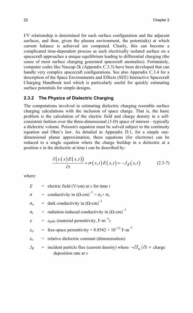
2.3.2 The Physics of Dielectric Charging The computations involved in estimating dielectric charging resemble surface charging calculations with the inclusion of space charge. That is, the basic problem is the calculation of the electric field and charge density in a self-consistent fashion over the three-dimensional (3-D) space of interest—typically a dielectric volume. Poisson's equation must be solved subject to the continuity equation and Ohm’s law. As detailed in Appendix D.1, for a simple one-dimensional planar approximation, these equations (for electrons) can be reduced to a single equation where the charge buildup in a dielectric at a position x in the dielectric at time t can be described by:

( ) ( )( ) ( ) ( ) ( )

,, , ,R

x E x tx t E x t J x t

tε

σ∂

+ = −∂

(2.3-7)

where:

E = electric field (V/cm) at x for time t

σ = conductivity in (Ω-cm)–1 = σo+ σr

σo = dark conductivity in (Ω-cm)–1

σr = radiation-induced conductivity in (Ω-cm)–1

ε = εoεr (material permittivity, F-m–1)

εo = free-space permittivity = 8.8542 × 10–12 F-m–1

εr = relative dielectric constant (dimensionless)

JR = incident particle flux (current density) where

−∂JR ∂x = charge deposition rate at x

Introduction to Physics of Charging and Discharging 23

Note in particular that the total current consists of the incident current JR (primary and secondary particles) and a conduction current σE driven by the electric field developed in the dielectric (the ohmic term). Integrating Eq. (2.3-7) in x across the dielectric layer then gives the variation of electric field in the dielectric at a given time. The results are stepped forward in time and the process repeated to give the changing electric field and charge density in the dielectric. As in the case of surface charging, computer codes such as NUMIT (Appendix C.2.7) and DICTAT (Appendix C.2.9) have been developed to carry out these computations and predict the buildup of electric field in the dielectric—when that field E exceeds the breakdown potential of the material, an arc discharge is possible.

2.4 Discharge Characteristics Charged spacecraft surfaces, environmentally caused or deliberately biased, can discharge, and the resulting transients can couple into electrical systems. A spacecraft in space may be considered to be a capacitor relative to the space plasma potential. The spacecraft, in turn, is divided into numerous other capacitors by the dielectric surfaces used for thermal control and for power generation. This system of capacitors can be charged at different rates depending upon incident fluxes, time constants, and spacecraft configuration effects.

The system of capacitors floats electrically with respect to the space plasma potential. This can give rise to unstable conditions in which charge can be lost from the spacecraft to space. While the exact conditions required for such breakdowns are not known, what is known is that breakdowns do occur, and it is hoped that conditions that lead to breakdowns can be bounded.

Breakdowns, or discharges, occur because charge builds up in spacecraft dielectric surfaces or between various surfaces on the spacecraft. Whenever this charge buildup generates an electric field that exceeds a breakdown threshold, charge may be released from the spacecraft to space or to an adjacent surface with a different potential. This charge release will continue until the electric field can no longer sustain an arc. Hence, the amount of charge released will be limited to the total charge stored in or on the dielectric at the discharge site. Charge loss or current to space or another surface causes the dielectric surface voltage (at least locally) to relax toward zero. Since the dielectric is coupled capacitively to the structure, the charge loss will also cause the structure potential to become less negative. In fact, the structure could become positive with respect to the space plasma potential. The exposed conductive surfaces of the spacecraft will then collect electrons from the environment (or attract back the emitted ones) to reestablish the structure potential required by the ambient

24 Chapter 2

conditions. The whole process for a conducting body to charge relative to space can take only a few milliseconds while, in contrast, differential charging between surfaces may take from a few seconds to hours to reach equilibrium. Multiple discharges can be produced if intensities remain high long enough to reestablish the conditions necessary for a discharge.

It is well known in the spacecraft solar array community that there can be a charge loss over an extended area of the dielectric (NASA TP-2361) [10]. This phenomenon is produced by the plasma cloud from a discharge sweeping over dielectric surfaces where the underlying conductor is electrically connected to the arc site. Charge loss from solar array arcs has been seen for distances of 2 meters (m) and more from the arc site and can involve capacitances of several hundreds of picofarads (pF) in the discharge depending on configuration. This phenomenon can produce area-dependent charge losses capable of generating currents of 4–5 amperes (A). The differential voltages necessary to produce this large charge-clean-off type of discharge may be as low as 1000 V on solar arrays dependent on the specific type of array, geometric configuration, or environment. In modeling the charged surfaces swept free of charge by an arc, one should assume that all areas with substrates directly electrically connected to the arc site and with a line-of-sight to the arc site will be discharged and calculate the arc energy accordingly.

Because sunlight tends to charge all illuminated surfaces a few volts positive relative to the ambient plasma and shaded dielectric surfaces may charge strongly negatively, differential charging is likely to occur between sunlit and shadowed surfaces. Since breakdowns are believed to be related to differential charging, they can occur during sunlit charging events. Entering and exiting an eclipse, in contrast, results in a change in absolute charging for all surfaces except those weakly capacitively coupled to the structure (capacitance to structure less than that of spacecraft to space, normally <2 × 10-10 F). Differential charging in eclipse develops slowly and depends upon differences in secondary yield. In the following paragraphs, each of the identified breakdown mechanisms is summarized.

2.4.1 Dielectric Surface Breakdowns If either of the following criteria is exceeded, discharges can occur:

1. If electric fields reach a magnitude that exceeds the breakdown strength of the surrounding “empty” space, a discharge may occur [11]. A published rule of thumb [12] is that if dielectric surface voltages resulting from spacecraft surface charging are greater than ~500 V, positive relative to an adjacent exposed conductor a breakdown may

Introduction to Physics of Charging and Discharging 25

occur. In this document, we have adopted a more conservative 400 V differential voltage threshold of concern for ESD breakdown. This is not true for induced potentials such as from solar arrays or Langmuir probes; these should be analyzed separately. The physics of electric field breakdown in gases has been explained by Townsend (see, for example, [11]).

2. The interface between a visible surface dielectric and an exposed grounded conductor has an electric field greater than 105 V/cm (NASA TP-2361) [10]. Note that edges, points, gaps, seams, and imperfections in surface materials can increase electric fields and hence promote the probability of discharges. These items are not usually modeled and must be found by close inspection of the exterior surface specifications. In some cases, a plasma cloud generated by a micrometeorid/debris impact at the site could trigger the breakdown.

The first criterion can be exceeded by solar arrays in which the high secondary yield of the cover slide can result in surface voltages that are positive with respect to the metalized interconnects. This criterion can also apply to metalized dielectrics in which the metalized film, either by accident or design, is isolated from structure ground by a large or non-existent resistance (essentially only capacitively coupled). In the latter case, the dielectric can be charged to large negative voltages (when shaded), and the metal film will thus become more negative than the surrounding surfaces and act as a cathode or electron emitter.

In both of these conditions, stored charge is initially ejected to space in the discharge process. This loss produces a transient that can couple into the spacecraft structure and possibly into the electronic systems. Current returns from space to the exposed conductive areas of the spacecraft. Transient currents flow in the structure depending on the electrical characteristics. It is assumed that the discharge process will continue until the voltage gradient or electric field that began the process disappears. The currents flowing in the structure will damp out according to its resistance.

The computation of charge lost in any discharge is highly speculative at this time. Basically, charge loss can be considered to result from the depletion of two capacitors; namely, that stored in the spacecraft, which is charged to a specified voltage relative to space, and that stored in a limited region of the dielectric at the discharge site. The prediction of charge loss requires not only the calculation of voltages on the spacecraft, but a careful review by an experienced analyst as well.

26 Chapter 2

As a guide, the following charge loss categories are useful (as adapted from NASA TP-2361 [10]):

0 < Qlost < 0.5 µC—minor discharge

0.5 < Qlost < 2 µC—moderate discharge

2 < Qlost < 10 µC—severe discharge

Energy, voltage, or discharge considerations can also be quantified as a means to characterize the severity of a dielectric discharge (or discharge from an isolated conductor). Assuming a 500 pF discharge capacitance as default and using the Qlost criteria above in standard equations yields the following (Table 2-2):

Table 2-2. Rough magnitudes of surface ESD event parameters.

Size Q (C) C (F) V E(J) Minor, up to 500 nC 500 pF 1 kV 250 µJ Moderate, up to 2 µC 500 pF 4 kV 4 mJ Severe, up to 10 µC 500 pF 20 kV 100 mJ

2.4.2 Buried (Internal) Charge Breakdowns This section refers to the situation where charges have sufficient energy to penetrate slightly below the surface of a dielectric and are trapped. If the dielectric surface is maintained near zero potential because of photoelectron or secondary electron emission, strong electric fields may exist in the material. This can lead to electric fields inside the material large enough to cause breakdowns. Breakdown can occur whenever the internal electric field exceeds 2 × 105 V/cm (2 × 107

V/m, ~508 V/mil). Table 6-1, Section 6.1, lists the breakdown strength of some dielectric materials.

A layer of charge with 2.2 × 1011 e/cm2 will create a 2 × 107 V/m electric field in a material with a relative dielectric constant of 2. (E-field is proportional to charge and inversely proportional to the dielectric constant.)

2.4.3 Spacecraft-to-Space Breakdowns Spacecraft-to-space breakdowns are generally similar to dielectric surface breakdowns but involve only small discharges. It is assumed that a strong electric field exists on the spacecraft surfaces—usually because of a geometric interfacing of metals and dielectrics. This arrangement periodically triggers a breakdown of the spacecraft capacitor. Since this spacecraft-to-space

Introduction to Physics of Charging and Discharging 27

capacitance tends to be of the order of 2 × 10-10 F, these breakdown transients should be small and rapid. Based on an assumption of 2 kV breakdown, the resulting stored energy is minor, in accordance with Table 2-2.

2.5 Coupling Models Coupling model analyses must be used to determine the hazard to electronic systems from exterior discharge transients. In this section, techniques for computing the influence of exterior discharge transients on interior spacecraft systems are discussed.

2.5.1 Lumped-Element Modeling (LEM) LEMs have been used to define the surface charging response to environmental fluxes [13–16] and are currently used to predict interior structural currents resulting from surface discharges. The basic philosophy of a LEM is that spacecraft surfaces and structures can be treated as electrical circuit elements—resistance, inductance, and capacitance. The geometry of the spacecraft is considered only to group or lump areas into nodes within the electrical circuit in much the same way as surfaces are treated as nodes in thermal modeling. These models, therefore, can be made as simple or as complex as is considered necessary for the circumstances.

The LEMs for discharges assume that the structure current transient is generated by capacitive coupling to the discharge site and is transmitted in the structure by conduction only. An analog circuit network is constructed by taking into consideration the structure properties and the geometry. This network must consider the principal current flow paths from the discharge site to exposed conductor areas—the return path to space plasma ground. Discharge transients are initiated at regions in this network selected as being probable discharge sites by surface charging predictions or other means. Choosing values of resistance, capacitance, and inductance to space can control transient characteristics. Network computer transient circuit analysis programs such as ISPICE, the first commercial version of SPICE (Simulation Program with Integrated Circuit Emphasis), and SPICE2 can solve the resulting transients within the network.

LEMs developed to predict surface charging rely on the use of current input terms applied independently to surfaces. Since there are no terms relating the influence of charging by one area on the incoming flux to other areas, the predictions usually result in larger negative voltages than actually observed. Other modeling techniques that take these three dimensional (3-D) effects into account, such as is done in Nascap-2k (Appendix C.3.3), predict surface

28 Chapter 2

voltages closer to those measured. Here, Nascap-2K is the currently recommended analysis technique for surface charging.

2.5.2 Electromagnetic Coupling Models Numerous programs have been developed to study the effects of electromagnetic coupling on circuits. Such programs have been used to compute the effects of an electromagnetic pulse (EMP) and that of an arc discharge. One program, the Specification and Electromagnetic Compatibility Program (SEMCAP) [17] developed by TRW Incorporated (now Northrop-Grumman Space Technology or NGST), has successfully analyzed the effects of arc discharges on an actual spacecraft, the Voyager spacecraft.

References [1] M. Bodeau, “Going Beyond Anomalies to Engineering Corrective Action,

New IESD Guidelines Derived From A Root-Cause Investigation,” presented at The 2005 Space Environmental Effects Working Group Workshop, Aerospace Corp., El Segundo, California, 2005. See also Balcewicz et al. (1998) [19].

[2] M. Bodeau, “High Energy Electron Climatology that Supports Deep Charging Risk Assessment in GEO,” AIAA 2010-1608, The 48th AIAA Aerospace Sciences Meeting, Orlando, Florida, 2010. xxxxxxxxxxxxxxx A fine work with good concepts, explained and illustrated with actual space data and estimates of fluence accumulation versus material resistivity. He challenges the 0.1 pA/cm2 and 10 hr flux integration guidelines.

[3] A. R. Frederickson, E. G. Holeman, and E. G. Mullen, “Characteristics of Spontaneous Electrical Discharges of Various Insulators in Space Radiation,” IEEE Transactions on Nuclear Science, vol. 39, no. 6, pp. 1773–1782, December 1992. xxxxxxxxxxxxxxxxxxxxxxxxxxxxxx This document is a description of the best-known attempt to quantify internal charging effects on orbit by means of a well-thought-out experiment design. The results were not all that the investigators had hoped, but the data are excellent and very good conclusions can be reached from the data in spite of the investigators’ concerns.

[4] J. I. Vette, The AE-8 Trapped Electron Model Environment, NSSDC/WDC-A-R&S, Report 91-24 National Space Science Data Center, Goddard, Maryland, November 1991.

[5] H. B. Garrett, “Review of Quantitative Models of the 0 to 100 keV Near-Earth Plasma,” Reviews of Geophysics and Space Physics, vol. 17, no. 3, pp. 397–416, 1979.

Introduction to Physics of Charging and Discharging 29

[6] D. Hastings and H. B. Garrett, Spacecraft-Environment Interactions, Atmospheric and Space Science Series, A. J. Dessler, Ed., Cambridge University Press, Cambridge, England, 292 pages, 1996. This is a college text on the subject. It contains additional reading for the space environment and interactions with spacecraft in its section 4.

[7] J. G. Roederer, Dynamics of Geomagnetically Trapped Radiation, Springer-Verlag, New York, New York, 166 pages, 1970.

[8] H. B. Garrett, Guide to Modeling Earth's Trapped Radiation Environment, AIAA G-083-1999, ISBN 1-56347-349-6, American Institute of Aeronautics and Astronautics, Reston, Virginia, 55 pages, 1999.

[9] H. B. Garrett, “The Charging of Spacecraft Surfaces,” Reviews of Geophysics and Space Physics, vol. 19, no. 4, pp. 577–616, November 1981. A nice summary paper, with numerical examples and many illustrations. This and Whipple (1981) [20] are two definitive papers on the subject, each covering slightly different aspects.

[10] C. K. Purvis, H. B. Garrett, A. C. Whittlesey, and N. J. Stevens, Design Guidelines for Assessing and Controlling Spacecraft Charging Effects, NASA Technical Paper 2361, National Aeronautics and Space Administration, September 1984.xxxxxxxxxxxxxxxxxxxxxxxxxxxxxxx This document has been widely used by practitioners of this art (usually EMC engineers or radiation survivability engineers) since its publication in 1984. Its contents are limited to surface charging effects. The contents are valid to this day for that purpose. NASA TP-2361 contents have been incorporated into this NASA-STD-4002, Rev A, with heavy editing. Many of the original details, especially time-variant and multiple-case versions of suggested environments, have been simplified into single worst-case environments in NASA-HDBK-4002, Revision A. Some background material has not been transferred into this document, so the original may still be of interest.

[11] M. S. Naidu and V. Kamaraju, High Voltage Engineering, Fourth Edition. Tata McGraw and Hill Publishing Company Limited, New Delhi, India, 2009. Townsend’s criteria for breakdown is described in this book.

[12] P. Coakley, Assessment of Internal ECEMP with Emphasis for Producing Interim Design Guidelines, AFWL-TN-86-28, Air Force Weapons Laboratory, June 1987. xxxxxxxxxxxxxxxxxxxxxxxxxxxxxxxxxxxxxxx This 63-page document (produced by JAYCOR, now part of L-3 Communications) was excellent in its day and still is a fine reference that

30 Chapter 2

should be on every ESD practitioner’s bookshelf. The design numbers from that document are very similar to those of this book.

[13] P. A. Robinson, Jr. and A. B. Holman, “Pioneer Venus Spacecraft Charging Model,” Proceedings of the Spacecraft Charging Technology Conference, AFGL-TR-77-0051/NASA TMX-73537, National Aero-nautics and Space Administration, pp. 297-308, 1977.

[14] G. T. Inouye, “Spacecraft Potentials in a Substorm Environment,” Spacecraft Charging by Magnetospheric Plasma. Vol. 42, A. Rosen, ed. MIT Press, Cambridge, Massachusetts, pp. 103–120, 1976.

[15] M. J. Massaro, T. Green, and D. Ling, “A Charging Model for Three-Axis Stabilized Spacecraft,” in Proceedings of the Spacecraft Charging Technology Conference, AFGL-TR-77-0051/NASA TMX-73537, National Aeronautics and Space Administration, pp. 237-270, 1977.

[16] M. J. Massaro and D. Ling, “Spacecraft Charging Results for the DSCS-III Satellite,” Spacecraft Charging Technology Conference, Air Force Geophysics Laboratory, Hanscom Air Force Base, Massachusetts, NASA Conference Publication 2071/AFGL TR-79-0082, National Aeronautics and Space Administration, pp. 158-178, 1979.

[17] R. Heidebrecht, SEMCAP Program Description, Version 7.4, TRW Electromagnetic Compatibility Department, Space Vehicles Division, TRW Systems Group, Redondo Beach, California, 1975.

[18] M. J. Berger, J. S. Coursey, M. A. Zucker, and J. Chang, Stopping-Power and Range Tables for Electrons, Protons, and Helium Ions, NISTIR 4999, National Institute of Standards and Technology, also available at http://www.nist.gov/physlab/data/star, April 26, 2010.

[19] P. Balcewicz, J. M. Bodeau, M. A. Frey, P. L. Leung, and E. J. Mikkelson, “Environmental On-Orbit Anomaly Correlation Efforts at Hughes,” 6th Spacecraft Charging Technology Conference Proceedings. AFRL-VS-TR-20001578. pp. 227–230, 1998.

[20] E. C. Whipple, “Potentials of Surfaces in Space,” Reports on Progress in Physics, vol. 44, pp. 1197–1250, 1981. xxxxxxxxxxxxxxxxxxxxxxxxxx Nice summary paper. Emphasis is on total charging and not internal charging, but good for physics background. This and Garrett (1981) [9] are the two definitive papers on that subject, each covering slightly different aspects.