
Chapter 2 : IDF-relationships and design storms · 2006-11-28 · Chapter 2 : IDF-relationships and...
28
Chapter 2 : IDF-relationships and design storms 2.1 Chapter 2 : IDF-relationships and design storms In this chapter the characterisation of the ‘mean’ rainfall is worked out based on Intensity/Duration/Frequency-relationships (IDF-relationships). New IDF-relationships are developed making optimal use of new methodologies and the current computer technology (paragraph 2.1). The new IDF-relationships are then compared with earlier (in Flanders) used design rainfall (paragraph 2.2). Furthermore, the simplification into mean rainfall input for sewer system calculations is worked out, which leads to composite design storms (paragraph 2.3). These composite storms have been set up for three different applications as there are : combined sewer system design (original application), hydrological calculations for long storm durations (paragraph 2.3.4) and modelling the influence of rain water storage tanks (paragraph 2.3.5). The applicability of these single storms and the accuracy of the obtained results is discussed in chapter 5 for the design calculations and in chapter 6 for the impact calculations. 2.1 IDF-relationships 2.1.1 The physical link with the design : the concentration time The use of rainfall Intensity/Duration/Frequency-relationships (IDF-relationships) has been standard practice for many decades for the design of sewer systems and other hydraulic structures. The IDF-relationships give an idea about the frequency or return period of a mean rainfall intensity or rainfall volume that can be expected within a certain period, i.e. the storm duration. In this sense the storm duration is an artificial parameter that can comprise any part of a rainfall event. IDF-relationships are certainly not old fashioned. Even in this computer age they provide a lot of information on the rainfall and they can be used as a base for the determination of design storms. The reason is the physically based link between IDF-relationships and hydraulic design, i.e. the concentration time. The concentration time is the time the rainfall needs in order to travel from the remotest place in the catchment to the point in the sewer system where the design calculation is made [Chow, 1964]. For a sewer system this means that the concentration time is the sum of the inlet time (time that the water flows over the surface to the sewer system) and the flow time (time that the water flows through the sewer system from the point where it enters the system to the design point). There will be a contribution to the flow in the design point from the whole upstream catchment if the storm duration is at least equal to the concentration time. This means that for a certain (constant) rainfall intensity a maximum for the flow will be obtained at the
Transcript of Chapter 2 : IDF-relationships and design storms · 2006-11-28 · Chapter 2 : IDF-relationships and...
Chapter 2 : IDF-relationships and design storms 2.1
Chapter 2 : IDF-relationships and design storms
In this chapter the characterisation of the ‘mean’ rainfall is worked out based onIntensity/Duration/Frequency-relationships (IDF-relationships).New IDF-relationships are developed making optimal use of new methodologiesand the current computer technology (paragraph 2.1). The new IDF-relationshipsare then compared with earlier (in Flanders) used design rainfall (paragraph 2.2).Furthermore, the simplification into mean rainfall input for sewer systemcalculations is worked out, which leads to composite design storms (paragraph 2.3).These composite storms have been set up for three different applications as there are: combined sewer system design (original application), hydrological calculations forlong storm durations (paragraph 2.3.4) and modelling the influence of rain waterstorage tanks (paragraph 2.3.5). The applicability of these single storms and theaccuracy of the obtained results is discussed in chapter 5 for the design calculations andin chapter 6 for the impact calculations.
2.1 IDF-relationships
2.1.1 The physical link with the design : the concentration time
The use of rainfall Intensity/Duration/Frequency-relationships (IDF-relationships)has been standard practice for many decades for the design of sewer systems and otherhydraulic structures. The IDF-relationships give an idea about the frequency orreturn period of a mean rainfall intensity or rainfall volume that can be expectedwithin a certain period, i.e. the storm duration. In this sense the storm duration isan artificial parameter that can comprise any part of a rainfall event. IDF-relationshipsare certainly not old fashioned. Even in this computer age they provide a lot ofinformation on the rainfall and they can be used as a base for the determination ofdesign storms. The reason is the physically based link between IDF-relationshipsand hydraulic design, i.e. the concentration time.
The concentration time is the time the rainfall needs in order to travel from theremotest place in the catchment to the point in the sewer system where the designcalculation is made [Chow, 1964]. For a sewer system this means thatthe concentration time is the sum of the inlet time (time that the water flows over thesurface to the sewer system) and the flow time (time that the water flows through thesewer system from the point where it enters the system to the design point). There willbe a contribution to the flow in the design point from the whole upstream catchment ifthe storm duration is at least equal to the concentration time. This means that for acertain (constant) rainfall intensity a maximum for the flow will be obtained at the
The influence of rainfall and model simplification on combined sewer system design2.2
rainfall intensity (mm/h)
0
10
20
30
40
50
60
0 20 40 60 80 100 120 140time (minutes)
rainfall for a return period of 2 years
flattened over duration of 20 minutes
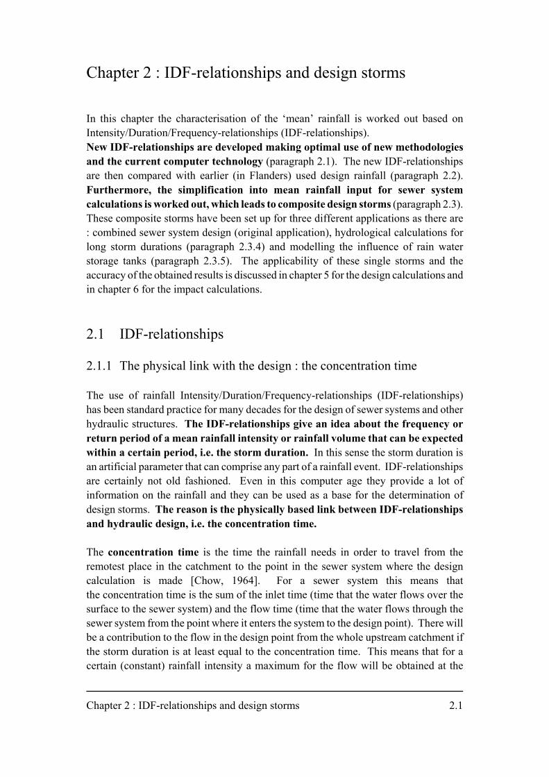
Figure 2.1 : Effect of a flattening over a concentration time of 20 minutes on the rainfall volumes for a return period of 2 years and storm durations
for 10, 20 and 30 minutes (see paragraph 2.1.5).
calculation point after a duration equal to the concentration time (if there is an equalcontribution of the whole catchment). Therefore, the duration of the storm equal to theconcentration time is the critical storm duration. The concentration time and thusalso the critical storm duration are specific parameters for each point. There is nosingle critical duration for the whole catchment. For the upstream points, short stormdurations will be critical and for more downstream points and larger catchments longerstorm durations will be critical.
For a certain frequency or return period the mean rainfall intensity over short durationswill be higher than over longer durations. In figure 2.1 the rainfall intensities areshown for durations of 10, 20 and 30 minutes for a return period of 2 years (seeparagraph 2.1.5). If these hyetographs are (equally) flattened over the sameconcentration time of 20 minutes, the storm with a duration of 20 minutes will lead toa maximum effect (figure 2.1). This means that for a certain return period thecritical storm duration (thus equal to the concentration time) will lead to themaximum effect. When a peaked rainfall event is flattened over the concentrationtime, the difference between the peak of the resulting hydrograph and the peak of theinitial rainfall event is equal to this concentration time. If this behaviour is inverted,it can be concluded that the concentration time can be approximated (from simulations)as the time difference between the peak rainfall and the peak flow in every point.
Chapter 2 : IDF-relationships and design storms 2.3
As the flow time over the surface and through the sewer system are dependent onthe flow velocity and the velocity is in some extent related to the rainfall input,the concentration time will actually not be a constant value for one specific point.This means that the concentration time in reality is not a static, but a dynamic parameter(i.e. a function of the rainfall intensity or flow : see paragraph 3.2.2).
2.1.2 The use of IDF-relationships in Flanders : short history
In 1985 Demarée published IDF-relationships. These IDF-relationships weredetermined based on the yearly maxima for the period 1934 - 1983 measured at theRoyal Meteorological Institute in Uccle (Belgium). These rainfall data were processedusing a Gumbel extreme value distribution with two parameters [Demarée, 1985].The use of yearly maxima was a simplification introduced to limit the process time andwork. With this method only IDF-relationships with a return period larger than 1 yearcan be derived. These IDF-relationships were used for about one decade for sewersystem design [Berlamont, 1987].
About one decade earlier, Laurant had already published IDF-relationships for Uccle[Laurant, 1976]. Laurant used the rainfall data measured at the same location(Royal Meteorological Institute in Uccle) for the period 1934 - 1973. These rainfalldata were analysed by direct fitting of curves to the calculated IDF-relationships(obtained by the monotone ranking method), without using any extreme valueestimation method. For that reason these IDF-relationships are less accurate for highreturn periods. Laurant extrapolated these IDF-relationships even for a return periodof 1000 years, but the accuracy for return periods higher than 10 years is low.The advantage of the IDF-relationships of Laurant is that they were determined also forreturn periods less than 2 years (i.e. for high frequencies). These IDF-relationshipshave never been prescribed for sewer system design, since the guidelines were in anearly stage of development prior to 1987 [De Backer, 1978].
Nowadays, powerful computers and new statistical methods are available to determinenew IDF-relationships without any restriction in data amounts or return periods.In 1994, the rainfall data for Uccle for the period 1967 - 1993 with a time step of10 minutes were made available in digital form by the Belgian Royal MeteorologicalInstitute (KMI) for research purposes. This was the start for a search for betterIDF-relationships and new design storms.
The influence of rainfall and model simplification on combined sewer system design2.4
2.1.3 Concept for the new IDF-relationships
For the development of the IDF-relationships in this study the distribution of rainfallvolumes (obtained by the monotonic ranking method) in a certain aggregation periodis determined for a wide range of aggregation periods. The aggregation period isthe period over which the rainfall intensities are summed up to obtain a mean rainfallintensity or a rainfall volume over a storm duration equal to the aggregation period.The minimum aggregation period is the time step of the original rainfall series,i.e. 10 minutes for the historical rainfall series of Uccle. For a specific aggregationperiod, a relationship between rainfall volume and exceedance frequency of that rainfallvolume is obtained from the cumulative probability distribution. This relationship isdetermined for every aggregation period that is a multiple of the rainfall time step.The intensity is the ratio of the rainfall volume to the aggregation period, i.e. stormduration. In practice this means that for a certain aggregation period the number ofrainfall volumes is counted, which exceed a specific threshold. This is called thepeak over threshold method. The return period (in [years]) for exceedance of thatthreshold value is then the total length of the original rainfall series (in [years]) dividedby the number of exceedances.
Two exceedances of a certain rainfall threshold can occur within a short period.This will not always lead to two different effects in the considered sewer system(e.g. two rainfall events which lead to only one flooding event or one overflow event).Therefore, an independency criterion has to be incorporated to distinguish dependantrainfall events which lead to the same effect. The problem with this criterion is itssubjectivity and its correlation with the design application. As the studied effects foreach application will be different, the criterion is application dependent. The rainfallvolumes over a certain aggregation level (storm duration) will be critical for thesepoints in a sewer system with a concentration time equal to the storm duration.Therefore, two rainfall events over this storm duration will lead to two different effects,if there is a period of at least the storm duration (concentration time) in between.This leads to an independency criterion which specifies that a rainfall volume is takeninto account if in a period equal to the aggregation period antecedent and posterior tothe considered rainfall volume no higher or equal rainfall volume occurs.Furthermore, two effects can be observed as dependent (thus as one event) if they aresituated close in time (e.g. two overflow events in a few hours). This is based more onthe psychological perception of the effect, than on an objectively defined criterion.For sewer system design, it can for instance be assumed that two effects areindependent if they do not occur on the same day or night. The independency criterionis then implemented as follows : two events are independent if in 12 hours before and12 hours after the event no higher (or equal) event occurs. This choice is made to limitthe subjectivity of the criterion, by preventing the need to make an arbitrary choice forthe time that a new day or night starts.
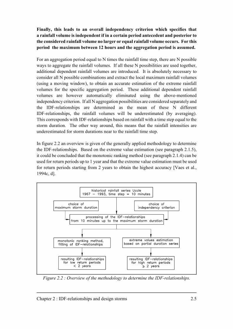
Chapter 2 : IDF-relationships and design storms 2.5
Figure 2.2 : Overview of the methodology to determine the IDF-relationships.
Finally, this leads to an overall independency criterion which specifies thata rainfall volume is independent if in a certain period antecedent and posterior tothe considered rainfall volume no larger or equal rainfall volume occurs. For thisperiod the maximum between 12 hours and the aggregation period is assumed.
For an aggregation period equal to N times the rainfall time step, there are N possibleways to aggregate the rainfall volumes. If all these N possibilities are used together,additional dependent rainfall volumes are introduced. It is absolutely necessary toconsider all N possible combinations and extract the local maximum rainfall volumes(using a moving window), to obtain an accurate estimation of the extreme rainfallvolumes for the specific aggregation period. These additional dependent rainfallvolumes are however automatically eliminated using the above-mentionedindependency criterion. If all N aggregation possibilities are considered separately andthe IDF-relationships are determined as the mean of these N differentIDF-relationships, the rainfall volumes will be underestimated (by averaging).This corresponds with IDF-relationships based on rainfall with a time step equal to thestorm duration. The other way around, this means that the rainfall intensities areunderestimated for storm durations near to the rainfall time step.
In figure 2.2 an overview is given of the generally applied methodology to determinethe IDF-relationships. Based on the extreme value estimation (see paragraph 2.1.5),it could be concluded that the monotonic ranking method (see paragraph 2.1.4) can beused for return periods up to 1 year and that the extreme value estimation must be usedfor return periods starting from 2 years to obtain the highest accuracy [Vaes et al.,1994c, d].
The influence of rainfall and model simplification on combined sewer system design2.6
rainfall intensity (mm/h)
0.1
1
10
100
10 100 1000storm
duration(minutes)
1 /year
2 /year
5 /year
10 /year
20 /year
Figure 2.3 : IDF-relationships for Uccle for frequencies between 1 and 20 p.a.using the monotone ranking technique for ‘independent’ rainfall volumes.
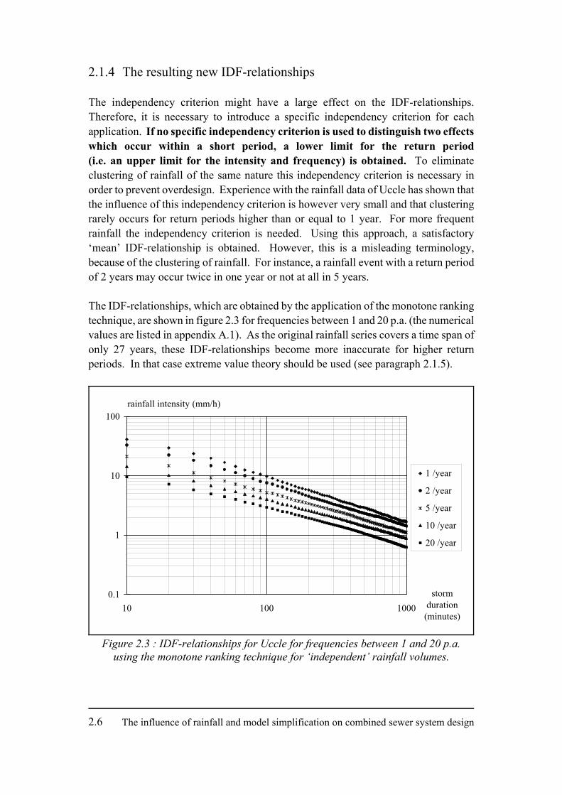
2.1.4 The resulting new IDF-relationships
The independency criterion might have a large effect on the IDF-relationships.Therefore, it is necessary to introduce a specific independency criterion for eachapplication. If no specific independency criterion is used to distinguish two effectswhich occur within a short period, a lower limit for the return period(i.e. an upper limit for the intensity and frequency) is obtained. To eliminateclustering of rainfall of the same nature this independency criterion is necessary inorder to prevent overdesign. Experience with the rainfall data of Uccle has shown thatthe influence of this independency criterion is however very small and that clusteringrarely occurs for return periods higher than or equal to 1 year. For more frequentrainfall the independency criterion is needed. Using this approach, a satisfactory‘mean’ IDF-relationship is obtained. However, this is a misleading terminology,because of the clustering of rainfall. For instance, a rainfall event with a return periodof 2 years may occur twice in one year or not at all in 5 years.
The IDF-relationships, which are obtained by the application of the monotone rankingtechnique, are shown in figure 2.3 for frequencies between 1 and 20 p.a. (the numericalvalues are listed in appendix A.1). As the original rainfall series covers a time span ofonly 27 years, these IDF-relationships become more inaccurate for higher returnperiods. In that case extreme value theory should be used (see paragraph 2.1.5).
Chapter 2 : IDF-relationships and design storms 2.7
(2.1)
(2.2)
(2.3)
To make IDF-relationships easier to use, they are often approximated by regressioncurves. For hydrological phenomena often a hyperbolic relation exists betweenthe amplitude and the duration, in this case the intensity i and the storm duration )t.The Talbot-Montana formula often gives good results (a1, a2 and a3 are regressionparameters) [Demarée, 1985] :
This formula leads to a linear relationship in a double logarithmic coordinate systemusing a constant shift a2 for the storm duration. For the IDF-relationships for Ucclethis formula does not give satisfactory regression results for all storm durations.Therefore, an extension with a second-order term in a double logarithmic coordinatesystem has been proposed in this study. This modified Talbot-Montana formula thenbecomes :
Or :
The extra regression parameter a4 is especially necessary to fit the small stormdurations. The regression coefficients are presented in table 2.1.
As the time step in the historical rainfall series is 10 minutes and this is also thesmallest storm duration considered, the question rises if the bending in the curves forsmall storm durations is not due to the averaging within the rainfall time step. In thatcase this bending should not be incorporated in the fitting, because an underestimationof the 10 minutes peak rainfall is obtained. This requires further attention, but theeffect of it phases out significantly for storm durations of 20, 30, ... minutes and this isthus of minor importance for design applications.
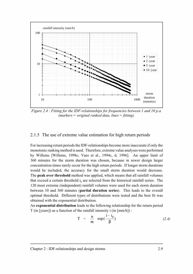
In figure 2.4 the fitting of the IDF-relationships for frequencies between 1 and 10 p.a.is shown for storm durations up to 720 minutes. The fitted IDF-relationships are listedin appendix A.2.
The influence of rainfall and model simplification on combined sewer system design2.8
frequency(p.a.)
regression coefficients
a1 a2 a3 a4
1 1582.844 14.36867 1.26778 - 0.094137
2 2517.828 17.37187 1.54020 - 0.156110
3 241.519 5.17747 0.83104 - 0.026011
4 134.960 3.59031 0.66541 0.006106
5 43.081 - 3.34774 0.30920 0.074643
6 48.737 - 1.33084 0.38552 0.056565
7 53.513 - 0.36559 0.44984 0.041244
8 55.995 0.84588 0.48095 0.035051
9 63.669 2.35176 0.54523 0.021303
10 47.347 0.74991 0.45944 0.038036
11 41.887 1.23952 0.42563 0.045611
12 38.843 1.17893 0.41168 0.048418
13 31.885 - 0.77606 0.35975 0.058012
14 33.058 0.30195 0.38236 0.053515
15 32.163 0.79145 0.38115 0.054113
16 35.931 2.34597 0.42473 0.046139
17 30.211 0.59111 0.37697 0.055318
18 29.247 1.41954 0.36850 0.058166
19 24.792 1.15932 0.31684 0.068966
20 21.208 - 0.52011 0.27076 0.078386
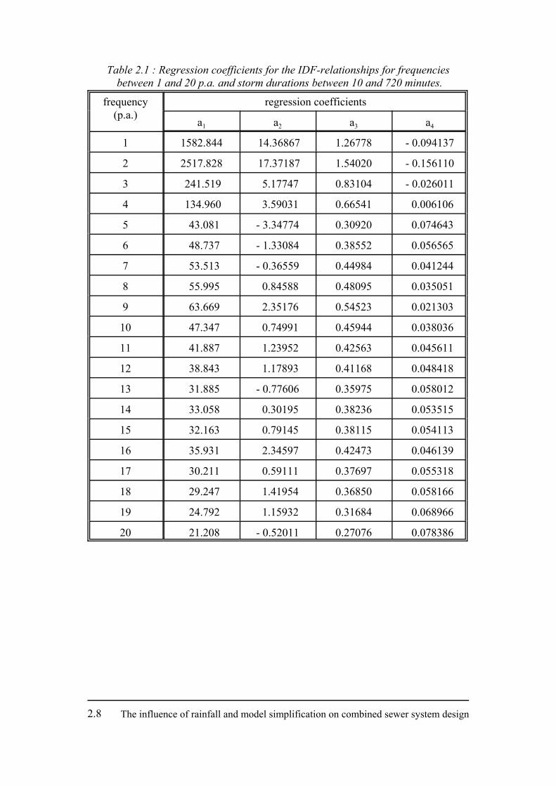
Table 2.1 : Regression coefficients for the IDF-relationships for frequencies between 1 and 20 p.a. and storm durations between 10 and 720 minutes.
Chapter 2 : IDF-relationships and design storms 2.9
rainfall intensity (mm/h)
1
10
100
10 100 1000
stormduration(minutes)
1 /year2 /year5 /year10 /year
Figure 2.4 : Fitting for the IDF-relationships for frequencies between 1 and 10 p.a.(markers = original ranked data, lines = fitting).
(2.4)
2.1.5 The use of extreme value estimation for high return periods
For increasing return periods the IDF-relationships become more inaccurate if only themonotonic ranking method is used. Therefore, extreme value analyses were performedby Willems [Willems, 1998c; Vaes et al., 1994c, d, 1996]. An upper limit of360 minutes for the storm duration was chosen, because in sewer design largerconcentration times rarely occur for the high return periods. If longer storm durationswould be included, the accuracy for the small storm duration would decrease.The peak over threshold method was applied, which means that all rainfall volumesthat exceed a certain threshold i0 are selected from the historical rainfall series. The120 most extreme (independent) rainfall volumes were used for each storm durationbetween 10 and 360 minutes (partial duration series). This leads to the overalloptimal threshold. Different types of distributions were tested and the best fit wasobtained with the exponential distribution.An exponential distribution leads to the following relationship for the return periodT (in [years]) as a function of the rainfall intensity i (in [mm/h]) :
The influence of rainfall and model simplification on combined sewer system design2.10
(2.5)
(2.6)
rainfall intensity (mm/h)
1
10
100
10 100 1000storm duration (minutes)
20 years10 years
5 years2 years
Figure 2.5 : IDF-relationships for return periods of 2, 5, 10 and 20 years (from bottom to top).
In this formula, n is the length of the historical rainfall series (= 27 years) and m thenumber of extreme rainfall volumes used (= 120). The two parameters of thisdistribution i0 (threshold intensity) and $ (mean intensity) are the characterisingintensities for the distribution (both in [mm/h]). Because these parameters behave asintensities, they can be fitted as a function of the storm duration )t (in [min]) using themodified Talbot-Montana formula (equation (2.2)), which leads to :
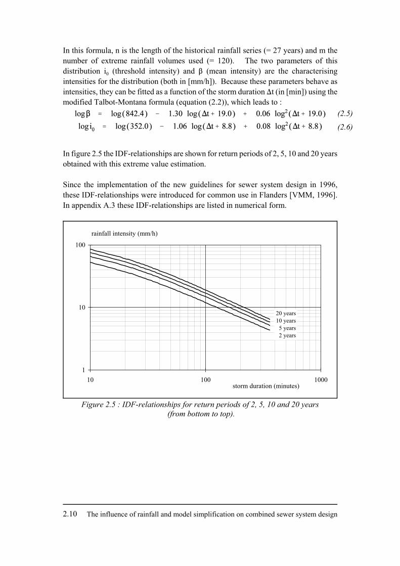
In figure 2.5 the IDF-relationships are shown for return periods of 2, 5, 10 and 20 yearsobtained with this extreme value estimation.
Since the implementation of the new guidelines for sewer system design in 1996,these IDF-relationships were introduced for common use in Flanders [VMM, 1996].In appendix A.3 these IDF-relationships are listed in numerical form.
Chapter 2 : IDF-relationships and design storms 2.11
( )
( )
log . .. log
. log . .
. .. log
. log .
iT
T t
TT
= ×+
− −
− ×+
+ +
9 68 08356 644 9
0 65 4387 0 00735
10 312 08356 644 9
0 9 46 37
∆(2.7)
2.2 Comparison with earlier design rainfall
2.2.1 IDF-relationships of Demarée
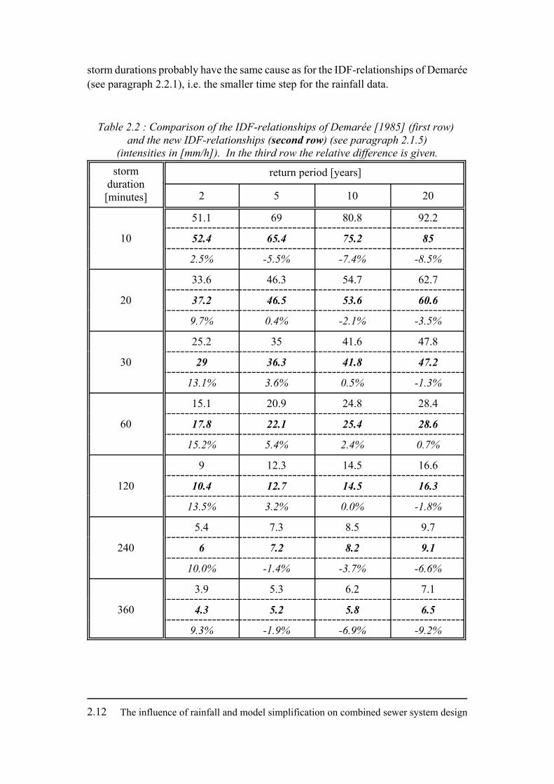
In the absence of powerful computer tools in the past, the method of periodic maximawas popular to determine the IDF-relationships, as was used by Demarée [1985] whoused yearly maxima. This method leads to an underestimation of the rainfall intensities(or an overestimation of the return periods), which has been shown theoretically[Demarée, 1985] and practically [Vaes et al., 1994c, d, 1996; Willems, 1998c].For larger return periods these differences become smaller. The disadvantage of themethod of yearly maxima is that it cannot lead to IDF-relationships for return periodssmaller than 2 years. In table 2.2 the comparison between the IDF-relationships ofDemarée [1985] and the new IDF-relationships (equations (2.4) to (2.6)) is shown.The underestimation of the rainfall intensities for low return periods using the yearlymaxima is obvious. Furthermore, smaller rainfall intensities are found with the newIDF-relationships for the short storm durations. This could point to the intrinsicaveraging within the time step of 10 minutes in the rainfall series used for the new IDF-relationships, because Demarée started from rainfall without this averaging (time stepaccuracy of about 1 minute). However, there are differences over the whole range ofstorm durations and return periods, which may be due to the difference in methodologyand different rainfall periods. The IDF-relationships of Demarée were commonly usedas block hyetographs for design calculations in Flanders. Also the IDF-relationshipsin the guidelines of 1987 were based on the work of Demarée [Berlamont, 1987].
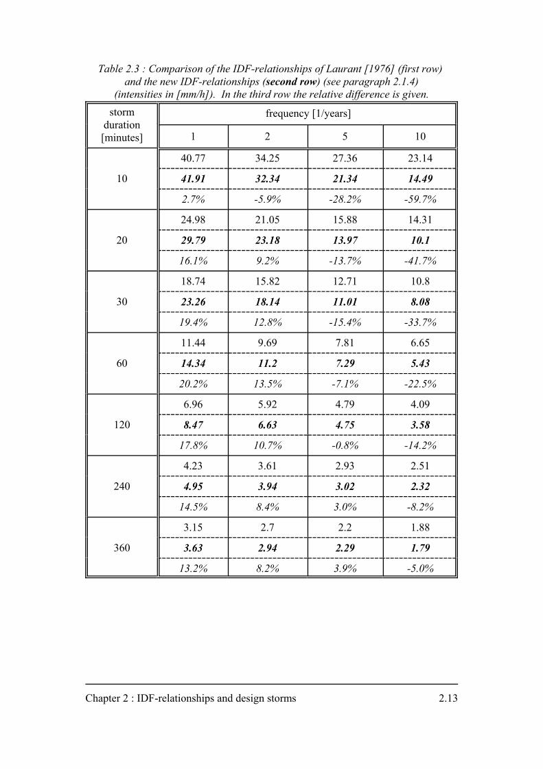
2.2.2 IDF-relationships of Laurant
In 1976, Laurant published IDF-relationships for Uccle, based on the rainfall series forthe period 1934-1973. To determine these IDF-relationships the monotonic rankingmethod was used. The IDF-relationships were determined for storm durations up to360 minutes. Then a formula was fit to the IDF-relationships [Laurant, 1976] :
in which i is the rainfall intensity in [mm/h], T is the return period in [year] and )t isthe storm duration in [min]. Some of the resulting IDF-relationships are listed intable 2.3. The differences with the new IDF-relationships are mainly due to thedifferent rainfall period which has been used and due to the differences in independencycriterion. The independency criterion of Laurant is less strict, which can lead to higherintensities, especially for more frequent rainfall events. The higher intensities for small
The influence of rainfall and model simplification on combined sewer system design2.12
stormduration[minutes]
return period [years]
2 5 10 20
10
51.1 69 80.8 92.2
52.4 65.4 75.2 85
2.5% -5.5% -7.4% -8.5%
20
33.6 46.3 54.7 62.7
37.2 46.5 53.6 60.6
9.7% 0.4% -2.1% -3.5%
30
25.2 35 41.6 47.8
29 36.3 41.8 47.2
13.1% 3.6% 0.5% -1.3%
60
15.1 20.9 24.8 28.4
17.8 22.1 25.4 28.6
15.2% 5.4% 2.4% 0.7%
120
9 12.3 14.5 16.6
10.4 12.7 14.5 16.3
13.5% 3.2% 0.0% -1.8%
240
5.4 7.3 8.5 9.7
6 7.2 8.2 9.1
10.0% -1.4% -3.7% -6.6%
360
3.9 5.3 6.2 7.1
4.3 5.2 5.8 6.5
9.3% -1.9% -6.9% -9.2%
Table 2.2 : Comparison of the IDF-relationships of Demarée [1985] (first row) and the new IDF-relationships (second row) (see paragraph 2.1.5)
(intensities in [mm/h]). In the third row the relative difference is given.
storm durations probably have the same cause as for the IDF-relationships of Demarée(see paragraph 2.2.1), i.e. the smaller time step for the rainfall data.
Chapter 2 : IDF-relationships and design storms 2.13
stormduration[minutes]
frequency [1/years]
1 2 5 10
10
40.77 34.25 27.36 23.14
41.91 32.34 21.34 14.49
2.7% -5.9% -28.2% -59.7%
20
24.98 21.05 15.88 14.31
29.79 23.18 13.97 10.1
16.1% 9.2% -13.7% -41.7%
30
18.74 15.82 12.71 10.8
23.26 18.14 11.01 8.08
19.4% 12.8% -15.4% -33.7%
60
11.44 9.69 7.81 6.65
14.34 11.2 7.29 5.43
20.2% 13.5% -7.1% -22.5%
120
6.96 5.92 4.79 4.09
8.47 6.63 4.75 3.58
17.8% 10.7% -0.8% -14.2%
240
4.23 3.61 2.93 2.51
4.95 3.94 3.02 2.32
14.5% 8.4% 3.0% -8.2%
360
3.15 2.7 2.2 1.88
3.63 2.94 2.29 1.79
13.2% 8.2% 3.9% -5.0%
Table 2.3 : Comparison of the IDF-relationships of Laurant [1976] (first row) and the new IDF-relationships (second row) (see paragraph 2.1.4)
(intensities in [mm/h]). In the third row the relative difference is given.
The influence of rainfall and model simplification on combined sewer system design2.14
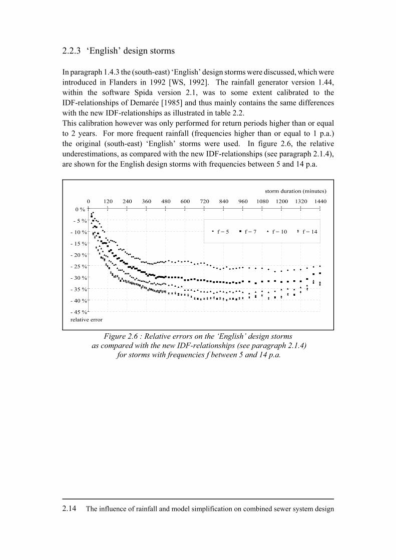
Figure 2.6 : Relative errors on the ‘English’ design storms as compared with the new IDF-relationships (see paragraph 2.1.4)
for storms with frequencies f between 5 and 14 p.a.
2.2.3 ‘English’ design storms
In paragraph 1.4.3 the (south-east) ‘English’ design storms were discussed, which wereintroduced in Flanders in 1992 [WS, 1992]. The rainfall generator version 1.44,within the software Spida version 2.1, was to some extent calibrated to theIDF-relationships of Demarée [1985] and thus mainly contains the same differenceswith the new IDF-relationships as illustrated in table 2.2.This calibration however was only performed for return periods higher than or equalto 2 years. For more frequent rainfall (frequencies higher than or equal to 1 p.a.)the original (south-east) ‘English’ storms were used. In figure 2.6, the relativeunderestimations, as compared with the new IDF-relationships (see paragraph 2.1.4),are shown for the English design storms with frequencies between 5 and 14 p.a.
Chapter 2 : IDF-relationships and design storms 2.15
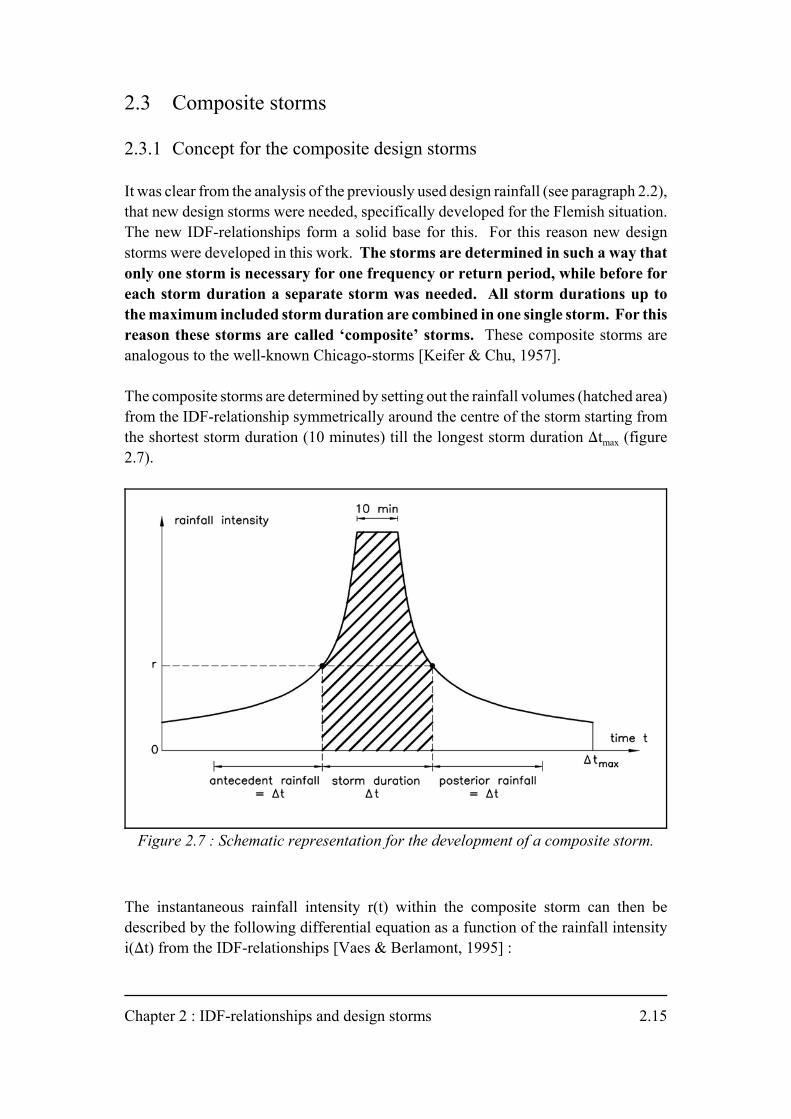
Figure 2.7 : Schematic representation for the development of a composite storm.
2.3 Composite storms
2.3.1 Concept for the composite design storms
It was clear from the analysis of the previously used design rainfall (see paragraph 2.2),that new design storms were needed, specifically developed for the Flemish situation.The new IDF-relationships form a solid base for this. For this reason new designstorms were developed in this work. The storms are determined in such a way thatonly one storm is necessary for one frequency or return period, while before foreach storm duration a separate storm was needed. All storm durations up tothe maximum included storm duration are combined in one single storm. For thisreason these storms are called ‘composite’ storms. These composite storms areanalogous to the well-known Chicago-storms [Keifer & Chu, 1957].
The composite storms are determined by setting out the rainfall volumes (hatched area)from the IDF-relationship symmetrically around the centre of the storm starting fromthe shortest storm duration (10 minutes) till the longest storm duration )tmax (figure2.7).
The instantaneous rainfall intensity r(t) within the composite storm can then bedescribed by the following differential equation as a function of the rainfall intensityi()t) from the IDF-relationships [Vaes & Berlamont, 1995] :
The influence of rainfall and model simplification on combined sewer system design2.16
(2.8)
(2.9)
rainfall intensity (mm/h)
0
10
20
30
40
50
0 1 2 3 4 5 6time (hour)
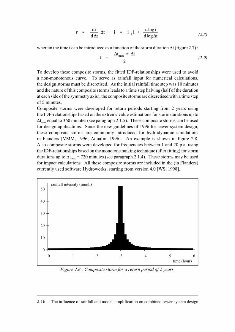
Figure 2.8 : Composite storm for a return period of 2 years.
wherein the time t can be introduced as a function of the storm duration )t (figure 2.7) :
To develop these composite storms, the fitted IDF-relationships were used to avoida non-monotonous curve. To serve as rainfall input for numerical calculations,the design storms must be discretised. As the initial rainfall time step was 10 minutesand the nature of this composite storms leads to a time step halving (half of the durationat each side of the symmetry axis), the composite storms are discretised with a time stepof 5 minutes.Composite storms were developed for return periods starting from 2 years usingthe IDF-relationships based on the extreme value estimations for storm durations up to)tmax equal to 360 minutes (see paragraph 2.1.5). These composite storms can be usedfor design applications. Since the new guidelines of 1996 for sewer system design,these composite storms are commonly introduced for hydrodynamic simulationsin Flanders [VMM, 1996; Aquafin, 1996]. An example is shown in figure 2.8.Also composite storms were developed for frequencies between 1 and 20 p.a. usingthe IDF-relationships based on the monotone ranking technique (after fitting) for stormdurations up to )tmax = 720 minutes (see paragraph 2.1.4). These storms may be usedfor impact calculations. All these composite storms are included in the (in Flanders)currently used software Hydroworks, starting from version 4.0 [WS, 1998].
Chapter 2 : IDF-relationships and design storms 2.17
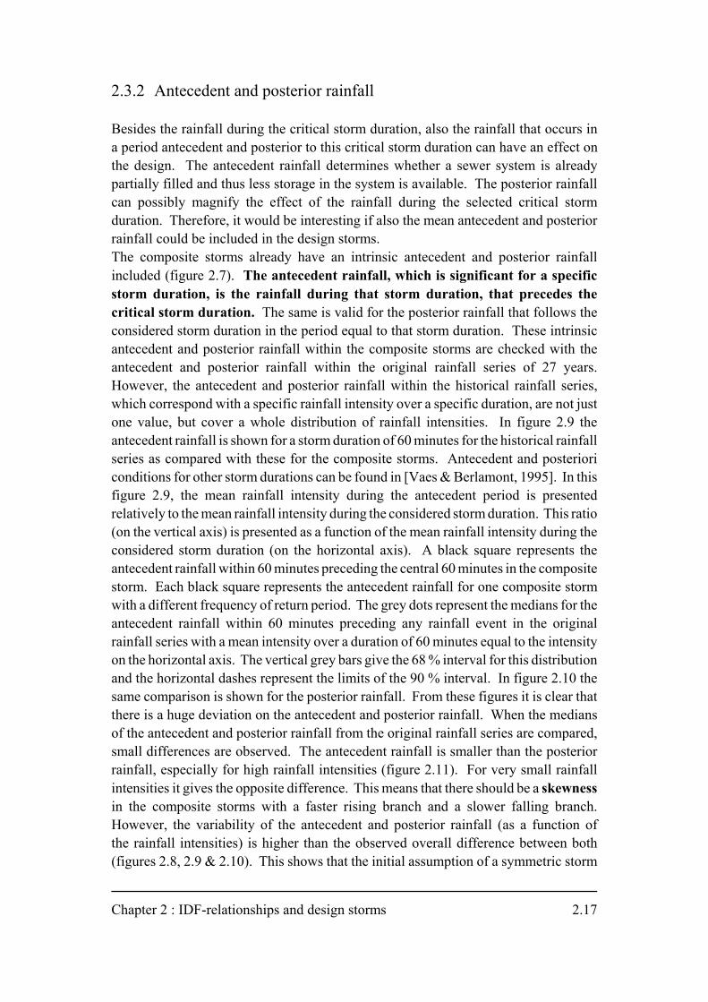
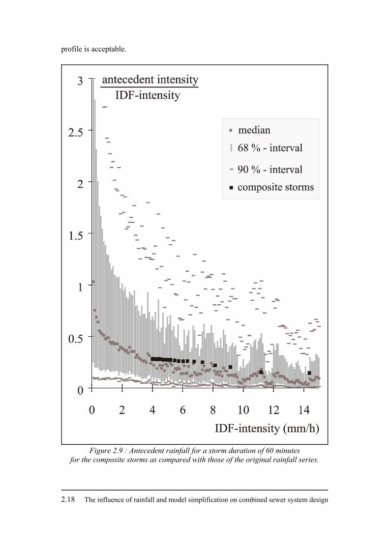
2.3.2 Antecedent and posterior rainfall
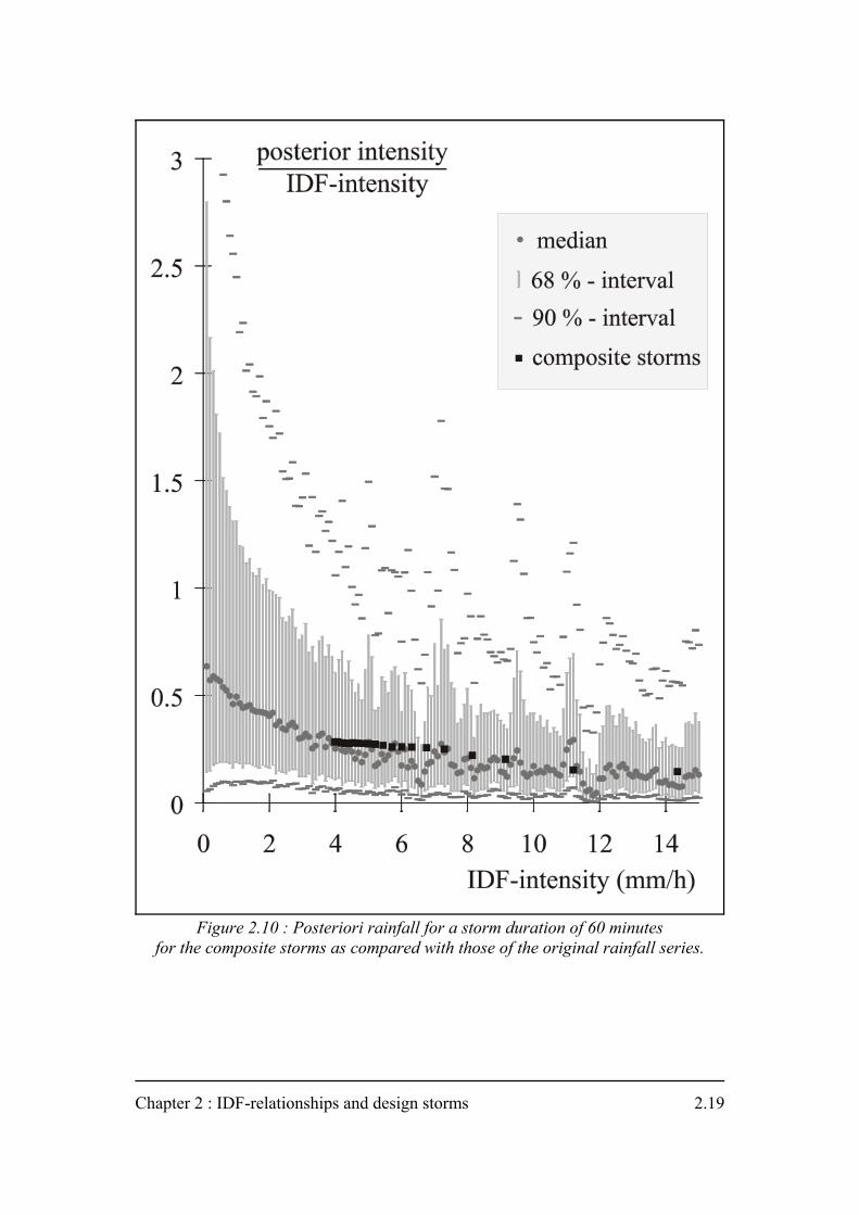
Besides the rainfall during the critical storm duration, also the rainfall that occurs ina period antecedent and posterior to this critical storm duration can have an effect onthe design. The antecedent rainfall determines whether a sewer system is alreadypartially filled and thus less storage in the system is available. The posterior rainfallcan possibly magnify the effect of the rainfall during the selected critical stormduration. Therefore, it would be interesting if also the mean antecedent and posteriorrainfall could be included in the design storms.The composite storms already have an intrinsic antecedent and posterior rainfallincluded (figure 2.7). The antecedent rainfall, which is significant for a specificstorm duration, is the rainfall during that storm duration, that precedes thecritical storm duration. The same is valid for the posterior rainfall that follows theconsidered storm duration in the period equal to that storm duration. These intrinsicantecedent and posterior rainfall within the composite storms are checked with theantecedent and posterior rainfall within the original rainfall series of 27 years.However, the antecedent and posterior rainfall within the historical rainfall series,which correspond with a specific rainfall intensity over a specific duration, are not justone value, but cover a whole distribution of rainfall intensities. In figure 2.9 theantecedent rainfall is shown for a storm duration of 60 minutes for the historical rainfallseries as compared with these for the composite storms. Antecedent and posterioriconditions for other storm durations can be found in [Vaes & Berlamont, 1995]. In thisfigure 2.9, the mean rainfall intensity during the antecedent period is presentedrelatively to the mean rainfall intensity during the considered storm duration. This ratio(on the vertical axis) is presented as a function of the mean rainfall intensity during theconsidered storm duration (on the horizontal axis). A black square represents theantecedent rainfall within 60 minutes preceding the central 60 minutes in the compositestorm. Each black square represents the antecedent rainfall for one composite stormwith a different frequency of return period. The grey dots represent the medians for theantecedent rainfall within 60 minutes preceding any rainfall event in the originalrainfall series with a mean intensity over a duration of 60 minutes equal to the intensityon the horizontal axis. The vertical grey bars give the 68 % interval for this distributionand the horizontal dashes represent the limits of the 90 % interval. In figure 2.10 thesame comparison is shown for the posterior rainfall. From these figures it is clear thatthere is a huge deviation on the antecedent and posterior rainfall. When the mediansof the antecedent and posterior rainfall from the original rainfall series are compared,small differences are observed. The antecedent rainfall is smaller than the posteriorrainfall, especially for high rainfall intensities (figure 2.11). For very small rainfallintensities it gives the opposite difference. This means that there should be a skewnessin the composite storms with a faster rising branch and a slower falling branch.However, the variability of the antecedent and posterior rainfall (as a function ofthe rainfall intensities) is higher than the observed overall difference between both(figures 2.8, 2.9 & 2.10). This shows that the initial assumption of a symmetric storm
The influence of rainfall and model simplification on combined sewer system design2.18
Figure 2.9 : Antecedent rainfall for a storm duration of 60 minutesfor the composite storms as compared with those of the original rainfall series.
profile is acceptable.
Chapter 2 : IDF-relationships and design storms 2.19
Figure 2.10 : Posteriori rainfall for a storm duration of 60 minutesfor the composite storms as compared with those of the original rainfall series.
The influence of rainfall and model simplification on combined sewer system design2.20
median antecedent or posterior intensityIDF-intensity
0
0.1
0.2
0.3
0.4
0.5
0.6
0.7
0.8
0 1 2 3 4 5 6 7 8 9 10 11 12 13 14IDF-intensity (mm/h)
antecedent condities
posteriori condities
Figure 2.11 : Comparison between the medians of the antecedent and the posteriorrainfall for a storm duration of 60 minutes.
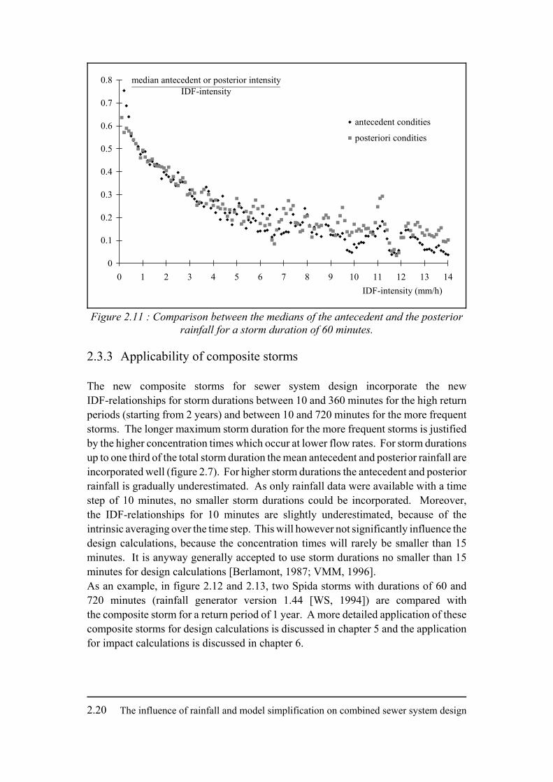
2.3.3 Applicability of composite storms
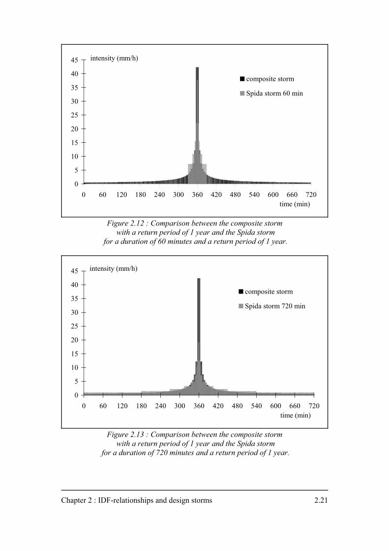
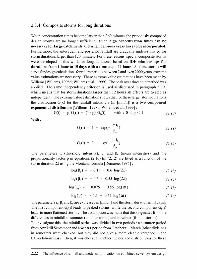
The new composite storms for sewer system design incorporate the newIDF-relationships for storm durations between 10 and 360 minutes for the high returnperiods (starting from 2 years) and between 10 and 720 minutes for the more frequentstorms. The longer maximum storm duration for the more frequent storms is justifiedby the higher concentration times which occur at lower flow rates. For storm durationsup to one third of the total storm duration the mean antecedent and posterior rainfall areincorporated well (figure 2.7). For higher storm durations the antecedent and posteriorrainfall is gradually underestimated. As only rainfall data were available with a timestep of 10 minutes, no smaller storm durations could be incorporated. Moreover,the IDF-relationships for 10 minutes are slightly underestimated, because of theintrinsic averaging over the time step. This will however not significantly influence thedesign calculations, because the concentration times will rarely be smaller than 15minutes. It is anyway generally accepted to use storm durations no smaller than 15minutes for design calculations [Berlamont, 1987; VMM, 1996].As an example, in figure 2.12 and 2.13, two Spida storms with durations of 60 and720 minutes (rainfall generator version 1.44 [WS, 1994]) are compared withthe composite storm for a return period of 1 year. A more detailed application of thesecomposite storms for design calculations is discussed in chapter 5 and the applicationfor impact calculations is discussed in chapter 6.
Chapter 2 : IDF-relationships and design storms 2.21
0
5
10
15
20
25
30
35
40
45
0 60 120 180 240 300 360 420 480 540 600 660 720time (min)
intensity (mm/h)
composite storm
Spida storm 720 min
Figure 2.13 : Comparison between the composite storm with a return period of 1 year and the Spida storm
for a duration of 720 minutes and a return period of 1 year.
0
5
10
15
20
25
30
35
40
45
0 60 120 180 240 300 360 420 480 540 600 660 720time (min)
intensity (mm/h)
composite storm
Spida storm 60 min
Figure 2.12 : Comparison between the composite storm with a return period of 1 year and the Spida storm
for a duration of 60 minutes and a return period of 1 year.
The influence of rainfall and model simplification on combined sewer system design2.22
(2.13)
(2.14)
(2.15)
(2.16)
(2.10)
(2.11)
(2.12)
2.3.4 Composite storms for long durations
When concentration times become larger than 360 minutes the previously composeddesign storms are no longer sufficient. Such high concentration times can benecessary for large catchments and when pervious areas have to be incorporated.Furthermore, the antecedent and posterior rainfall are gradually underestimated forstorm durations larger than 120 minutes. For these reasons, special composite stormswere developed in this work for long durations, based on IDF-relationships fordurations from 1 hour to 15 days with a time step of 1 hour. As these storms willserve for design calculations for return periods between 2 and even 2000 years, extremevalue estimations are necessary. These extreme value estimations have been made byWillems [Willems, 1998d; Willems et al., 1999]. The peak over threshold method wasapplied. The same independency criterion is used as discussed in paragraph 2.1.3,which means that for storm durations larger than 12 hours all effects are treated asindependent. The extreme value estimation shows that for these larger storm durationsthe distribution G(x) for the rainfall intensity i (in [mm/h]) is a two componentexponential distribution [Willems, 1998d; Willems et al., 1999] :
With :
The parameters i0 (threshold intensity), $a and $b (mean intensities) and theproportionality factor p in equations (2.10) till (2.12) are fitted as a function of thestorm duration )t using the Montana formula [Demarée, 1985] :
The parameters i0, $a and $b are expressed in [mm/h] and the storm duration is in [days].The first component Ga(i) leads to peaked storms, while the second component Gb(i)leads to more flattened storms. The assumption was made that this originates from thedifferences in rainfall in summer (thunderstorms) and in winter (frontal storms).To investigate this, the rainfall series was divided in two periods : a summer periodfrom April till September and a winter period from October till March (other divisionsin semesters were checked, but they did not give a more clear divergence in theIDF-relationships). Then, it was checked whether the derived distributions for these
Chapter 2 : IDF-relationships and design storms 2.23
(2.17)
(2.18)
(2.22)
(2.23)
(2.19)
( )β β ρ β ρa a b* = + −1 (2.20)
ρ = − − −
1 40 0113exp * .p (2.21)
f fw fs= + (2.24)
two periods, the summer distribution Gs(i) and the winter distribution Gw(i), can bewritten as a function of the previously found two exponential components :
This comparison showed that the winter distribution Gw(i) corresponds very well to thesecond component Gb(i). This means that pw is approximately 0. The summerdistribution Gs(i) remains a function of both exponential components Ga(i) and Gb(i) ofthe global distribution. The first component Ga(i) yields a dominant contribution to theshort storm durations and gradually decreases in importance for increasing stormdurations.A better estimation of the extreme rainfall events for the long durations is obtained ifthe component Ga(i) is slightly adjusted to Ga
*(i) [Willems, 1998d; Willems et al.,1999] :
With :
The return period T [years] can be calculated from the global distribution as :
Wherein : n is the number of years in the time series, i.e. 27 yearsm is the number of values above the threshold intensity i0
The superposition of the two seasonal distributions Gs(i) and Gw(i) must lead to thesame return period as for the global distribution G(i). The sum of the frequency ofa rainfall intensity in summer (fs = 1/Ts) and the frequency of the same rainfall intensityin winter (fw = 1/Tw) is equal to the frequency of that rainfall intensity in one year(f = 1/T) :
The influence of rainfall and model simplification on combined sewer system design2.24
(2.28)
(2.31)
(2.32)
1 1 1T Tw Ts= + (2.25)
( )
( )
Tsn
ms Gs in
m p Ga i ms m p Gb i
=−
=−
+ −
−
1
1 1
( )
* *( ) * ( )
(2.29)
( ) ( ) ( )Tw
nmw Gw i
nm ms Gb i
=−
=− −1 1( ) ( ) (2.30)
( )m G i m m p Ga i m p Gb i1 1− = − + −
( ) * *( ) * ( ) (2.26)
( ) ( )ms Gs i mw Gw i
m ms ps Ga i mms ps
mGb i
1 1
1
− + −
= − + −
( ) ( )
*( ) ( )(2.27)
or :
The return period T can be obtained analogously as illustrated for different boundaryconditions in paragraph 5.5.2 and figure 5.13.Using equations (2.23), (2.10), (2.12) and (2.19), equation (2.24) leads to :
Using equations (2.23), (2.17) and (2.18) the right hand side of the equation (2.24)leads to (in the assumption that pw = 0 and m = ms + mw) :
Equalising equations (2.26) and (2.27) leads to :
The return period for the summer storms then becomes (in [½ year]) :
and for the winter storms (in [½ year]) :
In these formulas the parameters m and ms are function of the storm duration via thethreshold intensity i0 (in [mm/h]) (equation 2.15) :
The matching IDF-relationships are listed in appendix A.4 for the summer storms andin appendix A.5 for the winter storms.
Chapter 2 : IDF-relationships and design storms 2.25
rainfall intensity (mm/h)
0
2
4
6
8
10
12
14
16
18
20
22
168 171 174 177 180 183 186 189 192time (hours)
winter storm
summer storm
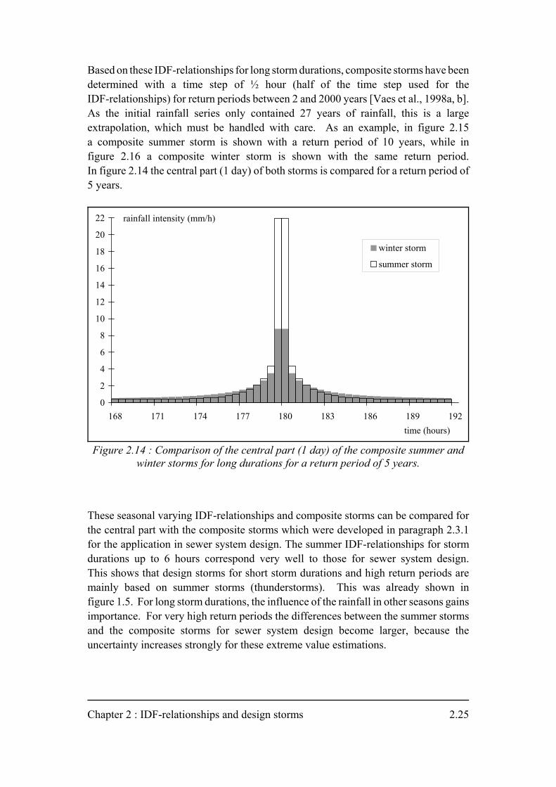
Figure 2.14 : Comparison of the central part (1 day) of the composite summer andwinter storms for long durations for a return period of 5 years.
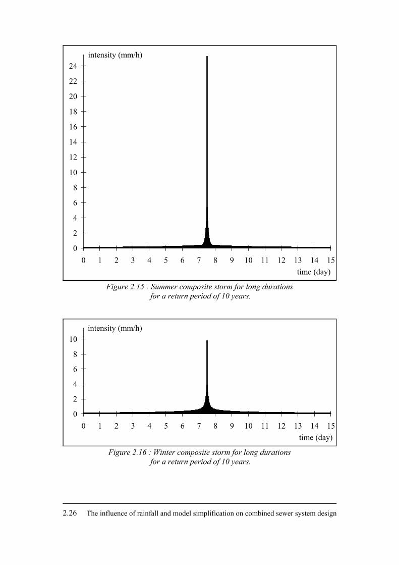
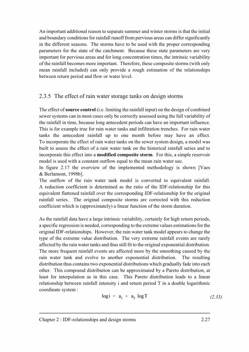
Based on these IDF-relationships for long storm durations, composite storms have beendetermined with a time step of ½ hour (half of the time step used for theIDF-relationships) for return periods between 2 and 2000 years [Vaes et al., 1998a, b].As the initial rainfall series only contained 27 years of rainfall, this is a largeextrapolation, which must be handled with care. As an example, in figure 2.15a composite summer storm is shown with a return period of 10 years, while infigure 2.16 a composite winter storm is shown with the same return period.In figure 2.14 the central part (1 day) of both storms is compared for a return period of5 years.
These seasonal varying IDF-relationships and composite storms can be compared forthe central part with the composite storms which were developed in paragraph 2.3.1for the application in sewer system design. The summer IDF-relationships for stormdurations up to 6 hours correspond very well to those for sewer system design.This shows that design storms for short storm durations and high return periods aremainly based on summer storms (thunderstorms). This was already shown infigure 1.5. For long storm durations, the influence of the rainfall in other seasons gainsimportance. For very high return periods the differences between the summer stormsand the composite storms for sewer system design become larger, because theuncertainty increases strongly for these extreme value estimations.
The influence of rainfall and model simplification on combined sewer system design2.26
intensity (mm/h)
0
2
4
6
8
10
12
14
16
18
20
22
24
0 1 2 3 4 5 6 7 8 9 10 11 12 13 14 15time (day)
Figure 2.15 : Summer composite storm for long durations for a return period of 10 years.
intensity (mm/h)
0
2
4
6
8
10
0 1 2 3 4 5 6 7 8 9 10 11 12 13 14 15time (day)
Figure 2.16 : Winter composite storm for long durations for a return period of 10 years.
Chapter 2 : IDF-relationships and design storms 2.27
(2.33)
An important additional reason to separate summer and winter storms is that the initialand boundary conditions for rainfall runoff from pervious areas can differ significantlyin the different seasons. The storms have to be used with the proper correspondingparameters for the state of the catchment. Because these state parameters are veryimportant for pervious areas and for long concentration times, the intrinsic variabilityof the rainfall becomes more important. Therefore, these composite storms (with onlymean rainfall included) can only provide a rough estimation of the relationshipsbetween return period and flow or water level.
2.3.5 The effect of rain water storage tanks on design storms
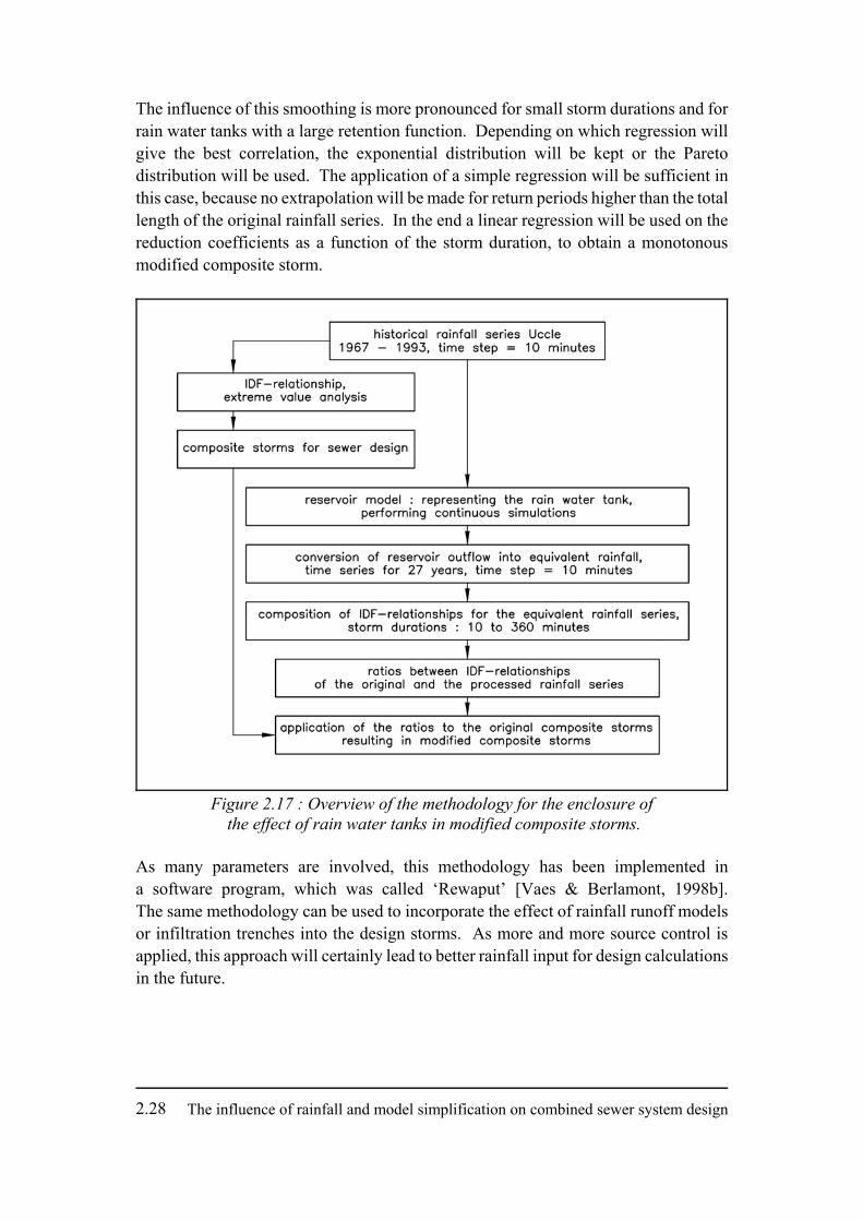
The effect of source control (i.e. limiting the rainfall input) on the design of combinedsewer systems can in most cases only be correctly assessed using the full variability ofthe rainfall in time, because long antecedent periods can have an important influence.This is for example true for rain water tanks and infiltration trenches. For rain watertanks the antecedent rainfall up to one month before may have an effect.To incorporate the effect of rain water tanks on the sewer system design, a model wasbuilt to assess the effect of a rain water tank on the historical rainfall series and toincorporate this effect into a modified composite storm. For this, a simple reservoirmodel is used with a constant outflow equal to the mean rain water use.In figure 2.17 the overview of the implemented methodology is shown [Vaes& Berlamont, 1998b].The outflow of the rain water tank model is converted to equivalent rainfall.A reduction coefficient is determined as the ratio of the IDF-relationship for thisequivalent flattened rainfall over the corresponding IDF-relationship for the originalrainfall series. The original composite storms are corrected with this reductioncoefficient which is (approximately) a linear function of the storm duration.
As the rainfall data have a large intrinsic variability, certainly for high return periods,a specific regression is needed, corresponding to the extreme values estimations for theoriginal IDF-relationships. However, the rain water tank model appears to change thetype of the extreme value distribution. The very extreme rainfall events are rarelyaffected by the rain water tanks and thus still fit to the original exponential distribution.The more frequent rainfall events are affected more by the smoothing caused by therain water tank and evolve to another exponential distribution. The resultingdistribution thus contains two exponential distributions which gradually fade into eachother. This compound distribution can be approximated by a Pareto distribution, atleast for interpolation as in this case. This Pareto distribution leads to a linearrelationship between rainfall intensity i and return period T in a double logarithmiccoordinate system :
The influence of rainfall and model simplification on combined sewer system design2.28
Figure 2.17 : Overview of the methodology for the enclosure of the effect of rain water tanks in modified composite storms.
The influence of this smoothing is more pronounced for small storm durations and forrain water tanks with a large retention function. Depending on which regression willgive the best correlation, the exponential distribution will be kept or the Paretodistribution will be used. The application of a simple regression will be sufficient inthis case, because no extrapolation will be made for return periods higher than the totallength of the original rainfall series. In the end a linear regression will be used on thereduction coefficients as a function of the storm duration, to obtain a monotonousmodified composite storm.
As many parameters are involved, this methodology has been implemented ina software program, which was called ‘Rewaput’ [Vaes & Berlamont, 1998b].The same methodology can be used to incorporate the effect of rainfall runoff modelsor infiltration trenches into the design storms. As more and more source control isapplied, this approach will certainly lead to better rainfall input for design calculationsin the future.