22

Chapter 2. Genome Anatomies

Learning outcomes 2.1. An Overview of Genome Anatomies

2.2. The Anatomy of the Eukaryotic Genome 2.3. The Anatomy of the Prokaryotic Genome 2.4. The Repetitive DNA Content of Genomes

Learning outcomes When you have read Chapter 2, you should be able to:

1. Draw diagrams illustrating the major differences between the genetic organizations of the genomes of humans, plants, insects, yeast and bacteria, and give an explanation for the C‐value paradox

2. Describe the DNA‐protein interactions that give rise to the chromatosome and the 30 nm chromatin fiber

3. State the functions of centromeres and telomeres and list their special structural features 4. Explain why chromosome banding patterns and the isochore model suggest that genes are not

evenly distributed in eukaryotic chromosomes 5. Outline the differences between the gene contents of different eukaryotic genomes and

explain, with examples, what is meant by ‘multigene family' 6. Describe the physical features and gene contents of mitochondrial and chloroplast genomes and

discuss the current hypothesis concerning the origins of organelle genomes 7. Describe the physical structure of the Escherichia coli genome and indicate the ways in which

this structure is and is not typical of other prokaryotes 8. Define, with examples, the term ‘operon' 9. Explain why prokaryotic genome sequences have complicated the species concept 10. Speculate on the content of the minimal prokaryotic genome and on the identity of

distinctiveness genes 11. Define the term ‘satellite DNA' and distinguish between satellite, minisatellite and microsatellite

DNA 12. Give examples of the various types of RNA and DNA transposons, and outline their transposition

pathways The human genome is by no means the only genome for which a complete or a draft sequence is available. By February 2001, when the draft human sequence was published, drafts were also available for the yeast Saccharomyces cerevisiae, the microscopic worm Caenorhabditis elegans, the fruit fly Drosophila melanogaster, the plant Arabidopsis thaliana, and one of the chromosomes of the malaria parasite Plasmodium falciparum. In addition, complete sequences had been obtained for over 30 microorganisms, including the bacteria Escherichia coli and Mycobacterium tuberculosis (Table 2.1). Work is progressing apace on the genomes of, among others, rice and the mouse, and plans are being made to start the chimpanzee genome project, the results of which will enable a direct comparison between the human genome and that of our closest non‐human relative. The completed and ongoing projects are revealing a great deal about how genomes are organized, including a number of unexpected discoveries that have taken molecular biologists by surprise. In this chapter we will survey the information that has arisen from genome projects and merge this information with the knowledge that was acquired in the pre‐genomic era of molecular biology.

2.1. An Overview of Genome Anatomies Biologists recognize that the living world comprises two types of organism (Figure 2.1):

1. Eukaryotes, whose cells contain membrane‐bound compartments, including a nucleus and organelles such as mitochondria and, in the case of plant cells, chloroplasts. Eukaryotes include animals, plants, fungi and protozoa.

2. Prokaryotes, whose cells lack extensive internal compartments. There are two very different groups of prokaryotes, distinguished from one another by characteristic genetic and biochemical features:

23

a. the bacteria, which include most of the commonly encountered prokaryotes such as the gram‐negatives (e.g. E. coli), the gram‐positives (e.g. Bacillus subtilis), the cyanobacteria (e.g. Anabaena) and many more;

b. the archaea, which are less well‐studied, and have mostly been found in extreme environments such as hot springs, brine pools and anaerobic lake bottoms.

Eukaryotes and prokaryotes have quite different types of genome and we must therefore consider them separately. Table 2.1. Examples of genomes for which a complete or draft sequence has been published

Species Size of genome (Mb)

Approximate number of genes

References

Eukaryotes

Arabidopsis thaliana (plant) 125 25 500 AGI (2000)

Caenorhabditis elegans (nematode worm)

97 19 000 CESC (1998)

Drosophila melanogaster (fruit fly) 180 13 600 Adams et al. (2000)

Homo sapiens (human) 3200 30 000–40 000 IHGSC (2001); Venter et al. (2001)

Saccharomyces cerevisiae (yeast) 12.1 5800 Goffeau et al. (1996)

Bacteria

Escherichia coli K12 4.64 4400 Blattner et al. (1997)

Mycobacterium tuberculosis H37Rv

4.41 4000 Cole et al. (1998)

Mycoplasma genitalium 0.58 500 Fraser et al. (1995)

Pseudomonas aeruginosa PA01 6.26 5700 Stover et al. (2000)

Streptococcus pneumoniae 2.16 2300 Tettelin et al. (2001)

Vibrio cholerae El Tor N16961 4.03 4000 Heidelberg et al. (2000)

Yersinia pestis CO92 4.65 4100 Parkhill et al. (2001)

Archaea

Archaeoglobus fulgidus 2.18 2500 Klenk et al. (1997)

Methanococcus jannaschii 1.66 1750 Bult et al. (1996)

For bacteria species, the strain designation (e.g. ‘K12') is given if specified by the group who sequenced the genome. With many bacterial species, different strains have different genome sizes and gene contents (Section 2.3.2).

Figure 2.1. Cells of eukaryotes (left) and prokaryotes (right). The top part of the figure shows a typical human cell and typical bacterium drawn to scale. The human cell is 10 μm in diameter and the bacterium is rod‐shaped with dimensions of 1 × 2 μm. The lower drawings show the internal structures of eukaryotic and prokaryotic cells. Eukaryotic cells are characterized by their membrane‐bound compartments, which are absent from prokaryotes. The bacterial DNA is contained in the structure called the nucleoid.

24

2.1.1. Genomes of eukaryotes Humans are fairly typical eukaryotes and the human genome is in many respects a good model for eukaryotic genomes in general. All of the eukaryotic nuclear genomes that have been studied are, like the human version, divided into two or more linear DNA molecules, each contained in a different chromosome; all eukaryotes also possess smaller, usually circular, mitochondrial genomes. The only general eukaryotic feature not illustrated by the human genome is the presence in plants and other photosynthetic organisms of a third genome, located in the chloroplasts. Although the basic physical structures of all eukaryotic nuclear genomes are similar, one important feature is very different in different organisms. This is genome size, the smallest eukaryotic genomes being less than 10 Mb in length, and the largest over 100 000 Mb. As can be seen in Table 2.2 , this size range coincides to a certain extent with the complexity of the organism, the simplest eukaryotes such as fungi having the smallest genomes, and higher eukaryotes such as vertebrates and flowering plants having the largest ones. This might appear to make sense as one would expect the complexity of an organism to be related to the number of genes in its genome ‐ higher eukaryotes need larger genomes to accommodate the extra genes. However, the correlation is far from precise: if it was, then the nuclear genome of the yeast S. cerevisiae, which at 12 Mb is 0.004 times the size of the human nuclear genome, would be expected to contain 0.004 × 35 000 genes, which is just 140. In fact the S. cerevisiae genome contains about 5800 genes.

Table 2.2. Sizes of eukaryotic genomes

Species Genome size (Mb)

Fungi

Saccharomyces cerevisiae 12.1

Aspergillus nidulans 25.4

Protozoa

Tetrahymena pyriformis 190

Invertebrates

Caenorhabditis elegans 97

Drosophila melanogaster 180

Bombyx mori (silkworm) 490

Strongylocentrotus purpuratus (sea urchin) 845

Locusta migratoria (locust) 5000

Vertebrates

Takifugu rubripes (pufferfish) 400

Homo sapiens 3200

Mus musculus (mouse) 3300

Plants

Arabidopsis thaliana (vetch) 125

Oryza sativa (rice) 430

Zea mays (maize) 2500

Pisum sativum (pea) 4800

Triticum aestivum (wheat) 16 000

Fritillaria assyriaca (fritillary) 120 000

For many years the lack of precise correlation between the complexity of an organism and the size of its genome was looked on as a bit of a puzzle, the so‐called C‐value paradox. In fact the answer is quite simple: space is saved in the genomes of less complex organisms because the genes are more closely packed together. The S. cerevisiae genome, the sequence of which was completed in 1996, illustrates this point, as we can see from the top two parts of Figure 2.2 , where the 50‐kb segment of the human genome that we looked at in Chapter 1 is compared with a 50‐kb segment of the yeast genome. The yeast genome segment, which comes from chromosome III (the first eukaryotic chromosome to be sequenced; Oliver et al., 1992), has the following distinctive features:

25

It contains more genes than the human segment. This region of yeast chromosome III contains 26 genes thought to code for proteins and two that code for transfer RNAs (tRNAs), short non‐coding RNA molecules involved in reading the genetic code during protein synthesis (Section 3.2.1). Relatively few of the yeast genes are discontinuous. In this segment of chromosome III none of the genes are discontinuous. In the entire yeast genome there are only 239 introns, compared with over 300 000 in the human genome. There are fewer genome‐wide repeats. This part of chromosome III contains a single long terminal repeat (LTR) element, called Ty2, and four truncated LTR elements called delta sequences. These five genome‐wide repeats make up 13.5% of the 50‐kb segment, but this figure is not entirely typical of the yeast genome as a whole. When all 16 yeast chromosomes are considered, the total amount of sequence taken up by genome‐wide repeats is only 3.4% of the total. In humans, the genome‐wide repeats make up 44% of the genome.

Figure 2.2. Comparison of the genomes of humans, yeast, fruit flies, maize and Escherichia coli. (A) is the 50‐kb segment of the human β T‐cell receptor locus shown in Figure 1.14 . This is compared with 50‐kb segments from the genomes of (B) Saccharomycescerevisiae (chromosome III; redrawn from Oliver et al., 1992); (C) Drosophila melanogaster (redrawn from Adams et al., 2000); (D) maize (redrawn from SanMiguel et al., 1996) and (E) E. coli K12 (redrawn from Blattner et al., 1997). See the text for more details. The picture that emerges is that the genetic organization of the yeast genome is much more economical than that of the human version. The genes themselves are more compact, having fewer introns, and the spaces between the genes are relatively short, with much less space taken up by genome‐wide repeats and other non‐coding sequences. The hypothesis that more complex organisms have less compact genomes holds when other species are examined. The third part of Figure 2.2 shows a 50‐kb segment of the fruit‐fly genome (Adams et al., 2000). If we agree that a fruit fly is more complex than a yeast cell but less complex than a human then we would expect the organization of the fruit‐fly genome to be intermediate between that of yeast and humans. This is what we see in Figure 2.2C , this 50‐kb segment of the fruit‐fly genome having 11 genes, more than in the human segment but fewer than in the yeast sequence. All of these genes are discontinuous, but seven have just one intron each. The picture is similar when the entire genome

26

sequences of the three organisms are compared (Table 2.3). The gene density in the fruit‐fly genome is intermediate between that of yeast and humans, and the average fruit‐fly gene has many more introns than the average yeast gene but still three times fewer than the average human gene.

Table 2.3. Compactness of the yeast, fruit‐fly and human genomes

Feature Yeast Fruit fly Human

Gene density (average number per Mb) 479 76 11

Introns per gene (average) 0.04 3 9

Amount of the genome that is taken up by genome‐wide repeats 3.4% 12% 44%

The comparison between the yeast, fruit‐fly and human genomes also holds true when we consider the genome‐wide repeats (see Table 2.3 ). These make up 3.4% of the yeast genome, about 12% of the fruit‐fly genome, and 44% of the human genome. It is beginning to become clear that the genome‐wide repeats play an intriguing role in dictating the compactness or otherwise of a genome. This is strikingly illustrated by the maize genome, which at 5000 Mb is larger than the human genome but still relatively small for a flowering plant. Only a few limited regions of the maize genome have been sequenced, but some remarkable results have been obtained, revealing a genome dominated by repetitive elements. Figure 2.2D shows a 50‐kb segment of this genome, either side of one member of a family of genes coding for the alcohol dehydrogenase enzymes (SanMiguel et al., 1996). This is the only gene in this 50‐kb region, although there is a second one, of unknown function, approximately 100 kb beyond the right‐hand end of the sequence shown here. Instead of genes, the dominant feature of this genome segment is the genome‐wide repeats. The majority of these are of the LTR element type, which comprise virtually all of the non‐coding part of the segment, and on their own are estimated to make up approximately 50% of the maize genome. It is becoming clear that one or more families of genome‐wide repeats have undergone a massive proliferation in the genomes of certain species. This may provide an explanation for the most puzzling aspect of the C‐value paradox, which is not the general increase in genome size that is seen in increasingly complex organisms, but the fact that similar organisms can differ greatly in genome size. A good example is provided by Amoeba dubia which, being a protozoan, might be expected to have a genome of 100–500 kb, similar to other protozoa such as Tetrahymena pyriformis (see Table 2.2). In fact the Amoeba genome is over 200 000 Mb. Similarly, we might guess that the genomes of crickets are similar in size to those of other insects, but these bugs have genomes of approximately 2000 Mb, 11 times that of the fruit fly. 2.1.2. Genomes of prokaryotes Prokaryotic genomes are very different from eukaryotic ones. There is some overlap in size between the largest prokaryotic and smallest eukaryotic genomes, but on the whole prokaryotic genomes are much smaller. For example, the E. coli K12 genome is just 4639 kb, two‐fifths the size of the yeast genome, and has only 4405 genes. The physical organization of the genome is also different in eukaryotes and prokaryotes. The traditional view has been that an entire prokaryotic genome is contained in a single circular DNA molecule. As well as this single ‘chromosome', prokaryotes may also have additional genes on independent smaller, circular or linear DNA molecules called plasmids (Figure 2.3). Genes carried by plasmids are useful, coding for properties such as antibiotic resistance or the ability to utilize complex compounds such as toluene as a carbon source, but plasmids appear to be dispensable ‐ a prokaryote can exist quite effectively without them. We now know that this traditional view of the prokaryotic genome has been biased by the extensive research on E. coli, which has been accompanied by the mistaken assumption that E. coli is a typical prokaryote. In fact, prokaryotes display a considerable diversity in genome organization, some having a unipartite genome, like E. coli, but others being more complex. Borrelia burgdorferi B31, for example, has a linear chromosome of 911 kb, carrying 853 genes, accompanied by 17 or 18 linear and circular molecules, which together contribute another 533 kb and at least 430 genes (Fraser et al., 1997). Multipartite genomes are now known in many other bacteria and archaea.

Figure 2.3. Plasmids are small circular DNA molecules that are found inside some prokaryotic cells.

27

In one respect, E. coli is fairly typical of other prokaryotes. After our discussion of eukaryotic gene organization, it will probably come as no surprise to learn that prokaryotic genomes are even more compact than those of yeast and other lower eukaryotes. We can see this fact illustrated in Figure 2.2E , which shows a 50‐kb segment of the E. coli K12 genome. It is immediately obvious that there are more genes and less space between them, with 43 genes taking up 85.9% of the segment. Some genes have virtually no space between them: thrA and thrB, for example, are separated by a single nucleotide, and thrC begins at the nucleotide immediately following the last nucleotide of thrB. These three genes are an example of an operon, a group of genes involved in a single biochemical pathway (in this case, synthesis of the amino acid threonine) and expressed in conjunction with one another. Operons have been used as model systems for understanding how gene expression is regulated (Section 9.3.1). In general, prokaryotic genes are shorter than their eukaryotic counterparts, the average length of a bacterial gene being about two‐thirds that of a eukaryotic gene, even after the introns have been removed from the latter (Zhang, 2000). Bacterial genes appear to be slightly longer than archaeal ones. Two other features of prokaryotic genomes can be deduced from Figure 2.2E . First, there are no introns in the genes present in this segment of the E. coli genome. In fact E. coli has no discontinuous genes at all, and it is generally believed that this type of gene structure is virtually absent in prokaryotes, the few exceptions occurring mainly among the archaea. The second feature is the infrequency of repetitive sequences. Most prokaryotic genomes do not have anything equivalent to the high‐copy‐number genome‐wide repeat families found in eukaryotic genomes. They do, however, possess certain sequences that might be repeated elsewhere in the genome, examples being the insertion sequences IS1 and IS186 that can be seen in the 50‐kb segment shown in Figure 2.2E . These are further examples of transposable elements, sequences that have the ability to move around the genome and, in the case of insertion elements, to transfer from one organism to another, even sometimes between two different species (see page 64). The positions of the IS1 and IS186 elements shown in Figure 2.2E refer only to the particular E. coli isolate from which this sequence was obtained: if a different isolate is examined then the IS sequences could well be in different positions or might be entirely absent from the genome. Most other prokaryotic genomes have very few repeat sequences ‐ there are virtually none in the 1.64 Mb genome of Campylobacter jejuni NCTC11168 (Parkhill et al., 2000b) ‐ but there are exceptions, notably the meningitis bacterium Neisseria meningitidis Z2491, which has over 3700 copies of 15 different types of repeat sequence, collectively making up almost 11% of the 2.18 Mb genome (Parkhill et al., 2000a).

2.2. The Anatomy of the Eukaryotic Genome We have already learnt that the human genome is split into two components: the nuclear genome and the mitochondrial genome (see Figure 1.1). This is the typical pattern for most eukaryotes, the bulk of the genome being contained in the chromosomes in the cell nucleus and a much smaller part located in the mitochondria and, in the case of photosynthetic organisms, in the chloroplasts. We will look first at the nuclear genome. 2.2.1. Eukaryotic nuclear genomes The nuclear genome is split into a set of linear DNA molecules, each contained in a chromosome. No exceptions to this pattern are known: all eukaryotes that have been studied have at least two chromosomes and the DNA molecules are always linear. The only variability at this level of eukaryotic genome structure lies with chromosome number, which appears to be unrelated to the biological features of the organism. For example, yeast has 16 chromosomes, four times as many as the fruit fly. Nor is chromosome number linked to genome size: some salamanders have genomes 30 times bigger than the human version but split into half the number of chromosomes. These comparisons are interesting but at present do not tell us anything useful about the genomes themselves; they are more a reflection of the non‐uniformity of the evolutionary events that have shaped genome architecture in different organisms. Packaging of DNA into chromosomes Chromosomes are much shorter than the DNA molecules that they contain: the average human chromosome has just under 5 cm of DNA. A highly organized packaging system is therefore needed to fit a DNA molecule into its chromosome. We must understand this packaging system before we start to think about how genomes function because the nature of the packaging has an influence on the processes involved in expression of individual genes (Section 8.2). The important breakthroughs in understanding DNA packaging were made in the early 1970s by a combination of biochemical analysis and electron microscopy. It was already known that nuclear DNA is associated with DNA‐binding proteins called histones but the exact nature of the association had not

28

been delineated. In 1973‐74 several groups carried out nuclease protection experiments on chromatin (DNA‐histone complexes) that had been gently extracted from nuclei by methods designed to retain as much of the chromatin structure as possible. In a nuclease protection experiment the complex is treated with an enzyme that cuts the DNA at positions that are not ‘protected' by attachment to a protein. The sizes of the resulting DNA fragments indicate the positioning of the protein complexes on the original DNA molecule (Figure 2.4). After limited nuclease treatment of purified chromatin, the bulk of the DNA fragments have lengths of approximately 200 bp and multiples thereof, suggesting a regular spacing of histone proteins along the DNA.

Figure 2.4. Nuclease protection analysis of chromatin from human nuclei. Chromatin is gently purified from nuclei and treated with a nuclease enzyme. On the left, the nuclease treatment is carried out under limiting conditions so that the DNA is cut, on average, just once in each of the linker regions between the bound proteins. After removal of the protein, the DNA fragments are analyzed by agarose gel electrophoresis (see Technical Note 2.1) and found to be 200 bp in length, or multiples thereof. On the right, the nuclease treatment proceeds to completion, so all the DNA in the linker regions is digested. The remaining DNA fragments are all 146 bp in length. The results show that in this form of chromatin, protein complexes are spaced along the DNA at regular intervals, one for each 200 bp, with 146 bp of DNA closely attached to each protein complex. In 1974 these biochemical results were supplemented by electron micrographs of purified chromatin, which enabled the regular spacing inferred by the protection experiments to be visualized as beads of protein on the string of DNA (Figure 2.5A). Further biochemical analysis indicated that each bead, or nucleosome, contains eight histone protein molecules, these being two each of histones H2A, H2B, H3 and H4. Structural studies have shown that these eight proteins form a barrel‐shaped core octamer with the DNA wound twice around the outside (Figure 2.5B). Between 140 and 150 bp of DNA (depending on the species) are associated with the nucleosome particle, and each nucleosome is separated by 50–70 bp of linker DNA, giving the repeat length of 190–220 bp previously shown by the nuclease protection experiments. As well as the proteins of the core octamer, there is a group of additional histones, all closely related to one another and collectively called linker histones. In vertebrates these include histones H1a‐e, H1°, H1t and H5. A single linker histone is attached to each nucleosome, to form the chromatosome, but the precise positioning of this linker histone is not known. Structural studies support the traditional model in which the linker histone acts as a clamp, preventing the coiled DNA from detaching from the nucleosome ( Figure 2.5C ; Zhou et al., 1998; Travers, 1999). However, other results suggest that, at least in some organisms, the linker histone is not located on the extreme surface of the nucleosome‐DNA assembly, as would be expected if it really were a clamp, but instead is inserted between the core octamer and the DNA (Pruss et al., 1995; Pennisi, 1996). The ‘beads‐on‐a‐string' structure shown in Figure 2.5A is thought to represent an unpacked form of chromatin that occurs only infrequently in living nuclei. Very gentle cell breakage techniques developed in the mid‐1970s resulted in a more condensed version of the complex, called the 30 nm fiber (it is approximately 30 nm in width). The exact way in which nucleosomes associate to form the 30 nm fiber is not known, but several models have been proposed, the most popular of which is the solenoid structure

29

shown in Figure 2.6 . The individual nucleosomes within the 30 nm fiber may be held together by interactions between the linker histones, or the attachments may involve the core histones, whose protein ‘tails' extend outside the nucleosome (see Figure 8.9 ). The latter hypothesis is attractive because chemical modification of these tails results in the 30 nm fiber opening up, enabling genes contained within it to be activated (Section 8.2.1).

Figure 2.5. Nucleosomes. (A) Electron micrograph of a purified chromatin strand showing the ‘beads‐on‐a‐string' structure. (Courtesy of Dr Barbara Hamkalo, University of California, Irvine.) (B) The model for the ‘beads‐on‐a‐string' structure in which each bead is a barrel‐shaped nucleosome with the DNA wound twice around the outside. Each nucleosome is made up of eight proteins: a central tetramer of two histone H3 and two histone H4 subunits, plus a pair of H2A‐H2B dimers, one above and one below the central tetramer (see Figure 8.9). (C) The precise position of the linker histone relative to the nucleosome is not known but, as shown here, the linker histone may act as a clamp, preventing the DNA from detaching from the outside of the nucleosome.

Figure 2.6. The solenoid model for the 30 nm chromatin fiber. In this model, the ‘beads‐on‐a‐string' structure of chromatin is condensed by winding the nucleosomes into a helix with six nucleosomes per turn. Higher levels of chromatin packaging are described in Section 8.1.2. The special features of metaphase chromosomes The 30 nm fiber is probably the major type of chromatin in the nucleus during interphase, the period between nuclear divisions. When the nucleus divides, the DNA adopts a more compact form of packaging, resulting in the highly condensed metaphase chromosomes that can be seen with the light microscope and which have the appearance generally associated with the word ‘chromosome' ( Figure 2.7 ). The metaphase chromosomes form at a stage in the cell cycle after DNA replication has taken place and so each one contains two copies of its chromosomal DNA molecule. The two copies are held together at the centromere, which has a specific position within each chromosome. Individual chromosomes can therefore be recognized because of their size and the location of the centromere relative to the two ends. Further distinguishing features are revealed when chromosomes are stained. There are a number of different staining techniques ( Table 2.4 ), each resulting in a banding pattern that is characteristic for a particular chromosome. This means that the set of chromosomes possessed by an organism can be represented as a karyogram, in which the banded appearance of each one is depicted. The human karyogram is shown in Figure 2.8 .

Figure 2.7. The typical appearance of a metaphase chromosome. Metaphase chromosomes are formed after DNA replication has taken place, so each one is, in effect, two chromosomes linked together at the centromere. The arms are called the chromatids. A telomere is the extreme end of a chromatid Both the DNA in the centromere regions, and the proteins attached to it, have special features. The nucleotide sequence of centromeric DNA is best understood in the plant Arabidopsis thaliana, whose amenity to genetic analysis has enabled the positions of the centromeres on the DNA sequence to be

30

located with some precision. Also, a special effort was made to sequence these centromeric regions, which are frequently excluded from draft genome sequences because of problems in obtaining an accurate reading through the highly repetitive structure that characterize these regions. Arabidopsis centromeres span 0.9–1.2 Mb of DNA and each one is made up largely of 180‐bp repeat sequences. In humans the equivalent sequences are 171 bp and are called alphoid DNA. Before the Arabidopsis sequences were obtained it was thought that these repeat sequences were by far the principal component of centromeric DNA. However, Arabidopsis centromeres also contain multiple copies of genome‐wide repeats, along with a few genes, the latter at a density of 7–9 per 100 kb compared with 25 genes per 100 kb for the non‐centromeric regions of Arabidopsis chromosomes (Copenhaver et al., 1999). The discovery that centromere DNA contains genes was a big surprise because it was thought that these regions were genetically inactive.

Figure 2.8. The human karyogram. The chromosomes are shown with the G‐banding pattern obtained after Giemsa staining. Chromosome numbers are given below each structure and the band numbers to the left. ‘rDNA' is a region containing a cluster of repeat units for the ribosomal RNA genes, which specify a type of non‐coding RNA (Section 3.2.1). ‘Constitutive heterochromatin' is very compact chromatin which has few or no genes (Section 8.1.2). Redrawn from Strachan and Read (1999).

31

The special centromeric proteins in humans include at least seven that are not found elsewhere in the chromosome (Warburton, 2001). One of these proteins, CENP‐A, is very similar to histone H3 and is thought to replace this histone in the centromeric nucleosomes. It is assumed that the small distinctions between CENP‐A and H3 confer special properties on centromeric nucleosomes, but exactly what these properties might be and how they relate to the function of the centromere is not yet known. Part of the function of the centromere itself is revealed by the electron microscope, which shows that in a dividing cell a pair of plate‐like kinetochores are present on the surface of the chromosome in the centromeric region. These structures act as the attachment points for the microtubules that radiate from the spindle pole bodies located at the nuclear surface and which draw the divided chromosomes into the daughter nuclei ( Figure 2.9 ). Part of the kinetochore is made up of alphoid DNA plus CENP‐A and other proteins, but its structure has not been described in detail (Vafa and Sullivan, 1997).

Figure 2.9. The role of the kinetochores during nuclear division. During the anaphase period of nuclear division (see Figures 5.14 and 5.15 ), individual chromosomes are drawn apart by the contraction of microtubules attached to the kinetochores. A second important part of the chromosome is the terminal region or telomere. Telomeres are important because they mark the ends of chromosomes and therefore enable the cell to distinguish a real end from an unnatural end caused by chromosome breakage ‐ an essential requirement because the cell must repair the latter but not the former. Telomeric DNA is made up of hundreds of copies of a repeated motif, 5′‐TTAGGG‐3′ in humans, with a short extension of the 3′ terminus of the double‐stranded DNA molecule (Figure 2.10). Two special proteins bind to the repeat sequences in human telomeres. These are called TRF1, which helps to regulate the length of the telomere, and TRF2, which maintains the single‐strand extension. If TRF2 is inactivated then this extension is lost and the two polynucleotides fuse together in a covalent linkage (van Steensel et al., 1998). Other telomeric proteins are thought to form a linkage between the telomere and the periphery of the nucleus, the area in which the chromosome ends are localized (Tham and Zakian, 2000). Still others mediate the enzymatic activity that maintains the length of each telomere during DNA replication. We will return to this last activity in Section 13.2.4: it critical to the survival of the chromosome and may be a key to understanding cell senescence and death.

Figure 2.10. Telomeres. The sequence at the end of a human telomere. The length of the 3′ extension is different in each telomere. See Section 13.2.4 for more details about telomeric DNA Where are the genes in a eukaryotic genome? In the previous section we learnt that Arabidopsis centromeres contain genes but at a lesser density than that in the rest of the chromosomes. This alerts us to the fact that the genes are not arranged evenly along the length of a chromosome. In most organisms, genes appear to be distributed more at less at random, with substantial variations in gene density at different positions within a chromosome. The average gene density in Arabidopsis is 25 genes per 100 kb, but even outside of the centromeres and telomeres the density varies from 1 to 38 genes per 100 kb, as illustrated in Figure 2.11 for the largest of the plant's five chromosomes. The same is true for human chromosomes, where the density ranges from 0 to 64 genes per 100 kb.

32

Figure 2.11. Gene density along the largest of the five Arabidopsis thaliana chromosomes. Chromosome 1, which is 29.1 Mb in length, is illustrated with the sequenced portions shown in red and the centromere and telomeres in blue. The gene map below the chromosome gives gene density in pseudocolor, from deep blue (low density) to red (high density). The density varies from 1 to 38 genes per 100 kb. Reprinted with permission from AGI (The Arabidopsis Genome Initiative), Nature, 408, 797–815. Copyright 2000 Macmillan Magazines Limited. The uneven gene distribution within human chromosomes was suspected for several years before the draft sequence was completed. There were two lines of evidence, one of which related to the banding patterns that are produced when chromosomes are stained. The dyes used in these procedures (see Table 2.4 ) bind to DNA molecules, but in most cases with preferences for certain base pairs. Giemsa, for example, has a greater affinity for DNA regions that are rich in A and T nucleotides. The dark G‐bands in the human karyogram (see Figure 2.8 ) are therefore thought to be AT‐rich regions of the genome. The base composition of the genome as a whole is 59.7% A + T so the dark G‐bands must have AT contents substantially greater than 60%. Cytogeneticists therefore predicted that there would be fewer genes in dark G‐bands because genes generally have AT contents of 45–50%. This prediction was confirmed when the draft genome sequence was compared with the human karyogram (IHGSC, 2001).

Table 2.4. Staining techniques used to produce chromosome banding patterns

Technique Procedure Banding pattern

G‐banding Mild proteolysis followed by staining with Giemsa

Dark bands are AT‐rich

Pale bands are GC‐rich

R‐banding Heat denaturation followed by staining with Giemsa

Dark bands are GC‐rich

Pale bands are AT‐rich

Q‐banding Stain with quinacrine Dark bands are AT‐rich

Pale bands are GC‐rich

C‐banding Denature with barium hydroxide and then stain with Giemsa

Dark bands contain constitutive heterochromatin (see Section 8.1.2)

The second line of evidence pointing to uneven gene distribution derived from the isochore model of genome organization (Gardiner, 1996). According to this model, the genomes of vertebrates and plants (and possibly of other eukaryotes) are mosaics of segments of DNA, each at least 300 kb in length, with each segment having a uniform base composition that differs from that of the adjacent segments. Support for the isochore model comes from experiments in which genomic DNA is broken into fragments of approximately 100 kb, treated with dyes that bind specifically to AT‐ or GC‐rich regions, and the pieces separated by density gradient centrifugation (Technical Note 2.2). When this experiment is carried out with human DNA, five fractions are seen, each representing a different isochore type with a distinctive base composition: two AT‐rich isochores, called L1 and L2, and three GC‐rich classes: H1, H2 and H3. The last of these, H3, is the least abundant in the human genome, making up only 3% of the total, but contains over 25% of the genes. This is a clear indication that genes are not distributed evenly through the human genome. The draft genome sequence suggests that the isochore theory over‐simplifies what is, in reality, a much more complex pattern of variations in base composition along the length of each human chromosome (IHGSC, 2001). But even if it turns out to be a misconception, the isochore theory has played an important role in helping molecular biologists of the pre‐sequence era to understand genome structure.

33

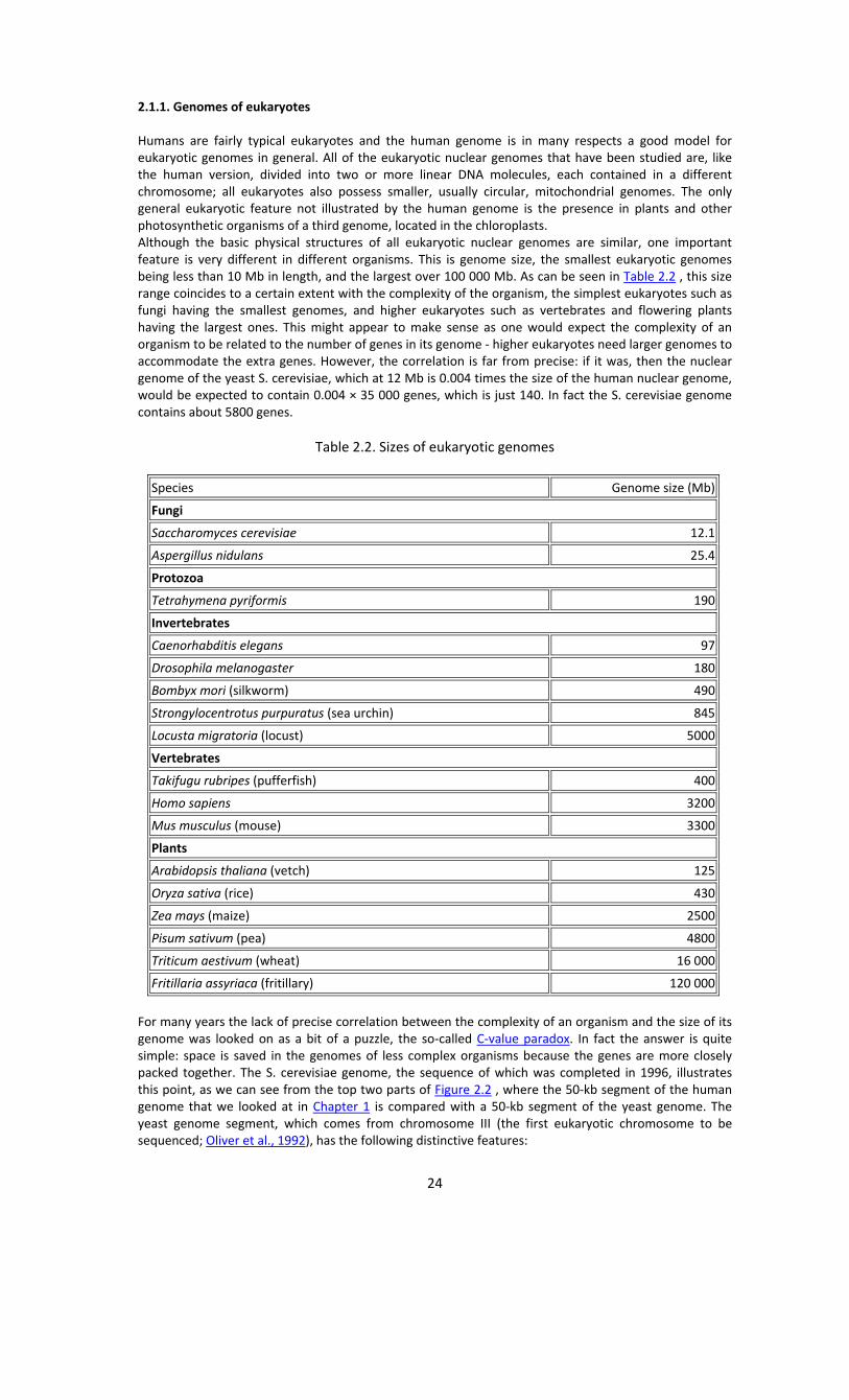
What genes are present in a eukaryotic genome? There are various ways to categorize the genes in a eukaryotic genome. One possibility is to classify the genes according to their function, as shown in Figure 1.18 (page 21) for the human genome. This system has the advantage that the fairly broad functional categories used in Figure 1.18 can be further subdivided to produce a hierarchy of increasingly specific functional descriptions for smaller and smaller sets of genes. The weakness with this approach is that functions have not yet been assigned to many eukaryotic genes, so this type of classification leaves out a proportion of the total gene set. A more powerful method is to base the classification not on the functions of genes but on the structures of the proteins that they specify. A protein molecule is constructed from a series of domains, each of which has a particular biochemical function. Examples are the zinc finger, which is one of several domains that enable a protein to bind to a DNA molecule (Section 9.1.4), and the ‘death domain', which is present in many proteins involved in apoptosis, the process of programmed cell death. Each domain has a characteristic amino acid sequence, perhaps not exactly the same sequence in every example of that domain, but close enough for the presence of a particular domain to be recognizable by examining the amino acid sequence of the protein. The amino acid sequence of a protein is specified by the nucleotide sequence of its gene, so the domains present in a protein can be determined from the nucleotide sequence of the gene that codes for that protein. The genes in a genome can therefore be categorized according to the protein domains that they specify. This method has the advantage that it can be applied to genes whose functions are not known and hence can encompass a larger proportion of the set of genes in a genome. Classification schemes based on gene function suggest that all eukaryotes possess the same basic set of genes, but that more complex species have a greater number of genes in each category. For example, humans have the greatest number of genes in all but one of the categories used in Figure 2.12 , the exception being ‘metabolism' where Arabidopsis comes out on top as a result of its photosynthetic capability, which requires a large set of genes not present in the other four genomes included in this comparison. This functional classification reveals other interesting features, notably that C. elegans has a relatively high number of genes whose functions are involved in cell‐cell signaling, which is surprising given that this organism has just 959 cells. Humans, who have 1013 cells, have only 250 more genes for cell‐cell signaling. In general, this type of analysis emphasizes the similarities between genomes, but does not reveal the genetic basis of the vastly different types of biological information contained in the genomes of, for example, fruit flies and humans. The domain approach holds more promise in this respect because it shows that the human genome specifies a number of protein domains that are absent from the genomes of other organisms, these domains including several involved in activities such as cell adhesion, electric couplings, and growth of nerve cells (Table 2.5). These functions are interesting because they are ones that we look on as conferring the distinctive features of vertebrates compared with other types of eukaryote.

Figure 2.12. Comparison of the gene catalogs of Saccharomyces cerevisiae, Arabidopsis thaliana, Caenorhabditis elegans, fruit fly and humans. Genes are categorized according to their function, as deduced from the protein domains specified by each gene. Redrawn from IHGSC (2001)

34

Table 2.5. Examples of protein domains specified by different genomes

Number of genes in the genome containing the domain

Domain Function Human Fruit fly

Caenorhabditis Arabidopsis Yeast

Zinc finger, C2H2 type

DNA binding 564 234 68 21 34

Zinc finger, GATA type

DNA binding 11 5 8 26 9

Homeobox Gene regulation during development

160 100 82 66 6

Death Programmed cell death 16 5 7 0 0

Connexin Electrical coupling between cells

14 0 0 0 0

Ephrin Nerve cell growth 7 2 4 0 0

Is it possible to identify a set of genes that are present in vertebrates but not in other eukaryotes? This analysis can only be done in an approximate way at present because only a few genome sequences are available. It currently appears that approximately one‐fifth to one‐quarter of the genes in the human genome are unique to vertebrates, and a further quarter are found only in vertebrates and other animals ( Figure 2.13 ).

Figure 2.13. Relationship between the human gene catalog and the catalogs of other groups of organism. The pie chart categorizes the human gene catalog according to the distribution of individual genes in other organisms. The chart shows, for example, that 22% of the human gene catalog is made up of genes that are specific to vertebrates, and that another 24% comprises genes specific to vertebrates and other animals. Genes are categorized according to their function, as deduced from the protein domains specified by each gene. Redrawn from IHGSC (2001). Families of genes Since the earliest days of DNA sequencing it has been known that multigene families ‐ groups of genes of identical or similar sequence ‐ are common features of many genomes. For example, every eukaryote that has been studied (as well as all but the simplest bacteria) has multiple copies of the genes for the non‐coding ribosomal RNAs (rRNAs; Section 3.2.1). This is illustrated by the human genome, which contains approximately 2000 genes for the 5S rRNA (so‐called because it has a sedimentation coefficient of 5S; see Technical Note 2.2), all located in a single cluster on chromosome 1. There are also about 280 copies of a repeat unit containing the 28S, 5.8S and 18S rRNA genes, grouped into five clusters of 50–70 repeats, one on each of chromosomes 13, 14, 15, 21 and 22 (see Figure 2.8). Ribosomal RNAs are components of the protein‐synthesizing particles called ribosomes, and it is presumed that their genes are present in multiple copies because there is a heavy demand for rRNA synthesis during cell division, when several tens of thousands of new ribosomes must be assembled. The rRNA genes are examples of ‘simple' or ‘classical' multigene families, in which all the members have identical or nearly identical sequences. These families are believed to have arisen by gene duplication,

35

with the sequences of the individual members kept identical by an evolutionary process that, as yet, has not been fully described (Section 15.2.1). Other multigene families, more common in higher eukaryotes than in lower eukaryotes, are called ‘complex' because the individual members, although similar in sequence, are sufficiently different for the gene products to have distinctive properties. One of the best examples of this type of multigene family are the mammalian globin genes. The globins are the blood proteins that combine to make hemoglobin, each molecule of hemoglobin being made up of two α‐type and two β‐type globins. In humans the α‐type globins are coded by a small multigene family on chromosome 16 and the β‐type globins by a second family on chromosome 11 (Figure 2.14). These genes were among the first to be sequenced, back in the late 1970s (Fritsch et al., 1980). The sequence data showed that the genes in each family are similar to one another, but by no means identical. In fact the nucleotide sequences of the two most different genes in the β‐type cluster, coding for the β‐ and ε‐globins, display only 79.1% identity. Although this is similar enough for both proteins to be β‐type globins, it is sufficiently different for them to have distinctive biochemical properties. Similar variations are seen in the α‐cluster. Why are the members of the globin gene families so different from one another? The answer was revealed when the expression patterns of the individual genes were studied. It was discovered that the genes are expressed at different stages in human development: for example, in the β‐type cluster ε is expressed in the early embryo, Gγ and Aγ (whose protein products differ by just one amino acid) in the fetus, and δ and β in the adult ( Figure 2.14 ). The different biochemical properties of the resulting globin proteins are thought to reflect slight changes in the physiological role that hemoglobin plays during the course of human development.

Figure 2.14. The human α‐ and β‐globin gene clusters. The α‐globin cluster is located on chromosome 16 and the β‐cluster on chromosome 11. Both clusters contain genes that are expressed at different developmental stages and each includes at least one pseudogene. Note that expression of the α‐type gene ξ2 begins in the embryo and continues during the fetal stage; there is no fetal‐specific α‐type globin. The θ pseudogene is expressed but its protein product is inactive. None of the other pseudogenes is expressed. For more information on the developmental regulation of the β‐globin genes, see Section 8.1.2. In some multigene families, the individual members are clustered, as with the globin genes, but in others the genes are dispersed around the genome. An example of a dispersed family is the five human genes for aldolase, an enzyme involved in energy generation, which are located on chromosomes 3, 9, 10, 16 and 17. The important point is that, even though dispersed, the members of the multigene family have sequence similarities that point to a common evolutionary origin. When these sequence comparisons are made it is sometimes possible to see relationships not only within a single gene family but also between different families. All of the genes in the α‐ and β‐globin families, for example, have some sequence similarity and are thought to have evolved from a single ancestral globin gene. We therefore refer to these two multigene families as comprising a single globin gene superfamily, and from the similarities between the individual genes we can chart the duplication events that have given rise to the series of genes that we see today (Section 15.2.1). 2.2.2. Eukaryotic organelle genomes Now we move out of the nucleus to examine the genomes present in the mitochondria and chloroplasts of eukaryotic cells. The possibility that some genes might be located outside of the nucleus ‐ extrachromosomal genes as they were initially called ‐ was first raised in the 1950s as a means of explaining the unusual inheritance patterns of certain genes in the fungus Neurospora crassa, the yeast

36

S. cerevisiae and the photosynthetic alga Chlamydomonas reinhardtii. Electron microscopy and biochemical studies at about the same time provided hints that DNA molecules might be present in mitochondria and chloroplasts. Eventually, in the early 1960s, these various lines of evidence were brought together and the existence of mitochondrial and chloroplast genomes, independent of and distinct from the nuclear genome, was accepted. Physical features of organelle genomes Almost all eukaryotes have mitochondrial genomes, and all photosynthetic eukaryotes have chloroplast genomes. Initially, it was thought that virtually all organelle genomes were circular DNA molecules. Electron microscopy studies had shown both circular and linear DNA in some organelles, but it was assumed that the linear molecules were simply fragments of circular genomes that had become broken during preparation for electron microscopy. We still believe that most mitochondrial and chloroplast genomes are circular, but we now recognize that there is a great deal of variability in different organisms. In many eukaryotes the circular genomes coexist in the organelles with linear versions and, in the case of chloroplasts, with smaller circles that contain subcomponents of the genome as a whole. The latter pattern reaches its extreme in the marine algae called dinoflagellates, whose chloroplast genomes are split into many small circles, each containing just a single gene (Zhang et al., 1999). We also now realize that the mitochondrial genomes of some microbial eukaryotes (e.g. Paramecium, Chlamydomonas and several yeasts) are always linear (Nosek et al., 1998). Copy numbers for organelle genomes are not particularly well understood. Each human mitochondrion contains about 10 identical molecules, which means that there are about 8000 per cell, but in S. cerevisiae the total number is probably smaller (less than 6500) even though there may be over 100 genomes per mitochondrion. Photosynthetic microorganisms such as Chlamydomonas have approximately 1000 chloroplast genomes per cell, about one‐fifth the number present in a higher plant cell. One mystery, which dates back to the 1950s and has never been satisfactorily solved, is that when organelle genes are studied in genetic crosses the results suggest that there is just one copy of a mitochondrial or chloroplast genome per cell. This is clearly not the case but indicates that our understanding of the transmission of organelle genomes from parent to offspring is less than perfect. Mitochondrial genome sizes are variable (Table 2.6) and are unrelated to the complexity of the organism. Most multicellular animals have small mitochondrial genomes with a compact genetic organization, the genes being close together with little space between them. The human mitochondrial genome (see Figure 1.22 ), at 16 569 bp, is typical of this type. Most lower eukaryotes such as S. cerevisiae ( Figure 2.15 ), as well as flowering plants, have larger and less compact mitochondrial genomes, with a number of the genes containing introns. Chloroplast genomes have less variable sizes (Table 2.6 ) and most have a structure similar to that shown in Figure 2.16 for the rice chloroplast genome.

Figure 2.15. The Saccharomyces cerevisiae mitochondrial genome. Because of their relatively small sizes, many mitochondrial genomes have been completely sequenced. In the yeast genome, the genes are more spaced out than in the human mitochondrial genome ( Figure 1.22 ) and some of the genes have introns. This type of organization is typical of many lower eukaryotes and plants. The yeast genome contains five additional open reading frames (not shown on this map) that have not yet been shown to code for functional gene products, and there are also several genes located within the introns of the discontinuous genes. Most of the latter code for maturase proteins involved in splicing the introns from the transcripts of these genes (Section 10.2.3). Abbreviations: ATP6, ATP8, ATP9, genes for ATPase subunits 6, 8 and 9, respectively; COI, COII, COIII, genes for cytochrome c oxidase subunits I, II and III, respectively; Cytb, gene for apocytochrome b; var 1, gene for a ribosome‐associated protein. Ribosomal RNA and transfer RNA are two types of non‐coding RNA (Section 3.2.1). The 9S RNA gene specifies the RNA component of the enzyme ribonuclease P (Section 10.2.2).

37

Table 2.6. Sizes of mitochondrial and chloroplast genomes

Species Type of organism Genome size (kb)

Mitochondrial genomes

Plasmodium falciparum Protozoan (malaria parasite) 6

Chlamydomonas reinhardtii Green alga 16

Mus musculus Vertebrate (mouse) 16

Homo sapiens Vertebrate (human) 17

Metridium senile Invertebrate (sea anemone) 17

Drosophila melanogaster Invertebrate (fruit fly) 19

Chondrus crispus Red alga 26

Aspergillus nidulans Ascomycete fungus 33

Reclinomonas americana Protozoa 69

Saccharomyces cerevisiae Yeast 75

Suillus grisellus Basidiomycete fungus 121

Brassica oleracea Flowering plant (cabbage) 160

Arabidopsis thaliana Flowering plant (vetch) 367

Zea mays Flowering plant (maize) 570

Cucumis melo Flowering plant (melon) 2500

Chloroplast genomes

Pisum sativum Flowering plant (pea) 120

Marchantia polymorpha Liverwort 121

Oryza sativa Flowering plant (rice) 136

Nicotiana tabacum Flowering plant (tobacco) 156

Chlamydomonas reinhardtii Green alga 195 The genetic content of organelle genomes Organelle genomes are much smaller than their nuclear counterparts and we therefore anticipate that their gene contents are much more limited, which is indeed the case. Again, mitochondrial genomes display the greater variability, gene contents ranging from five for the malaria parasite P. falciparum to 92 for the protozoan Reclinomonas americana (Table 2.7 ; Lang et al., 1997; Palmer, 1997a). All mitochondrial genomes contain genes for the non‐coding rRNAs and at least some of the protein components of the respiratory chain, the latter being the main biochemical feature of the mitochondrion. The more gene‐rich genomes also code for tRNAs, ribosomal proteins, and proteins involved in transcription, translation and transport of other proteins into the mitochondrion from the surrounding cytoplasm ( Table 2.7 ). Most chloroplast genomes appear to possess the same set of 200 or so genes, again coding for rRNAs and tRNAs, as well as ribosomal proteins and proteins involved in photosynthesis (see Figure 2.16 ). A general feature of organelle genomes emerges from Table 2.7 . These genomes specify some of the proteins found in the organelle, but not all of them. The other proteins are coded by nuclear genes, synthesized in the cytoplasm, and transported into the organelle. If the cell has mechanisms for transporting proteins into mitochondria and chloroplasts, then why not have all the organelle proteins specified by the nuclear genome? We do not yet have a convincing answer to this question, although it has been suggested that at least some of the proteins coded by organelle genomes are extremely hydrophobic and cannot be transported through the membranes that surround mitochondria and chloroplasts, and so simply cannot be moved into the organelle from the cytoplasm (Palmer, 1997b). The only way in which the cell can get them into the organelle is to make them there in the first place.

38

Table 2.7. Features of mitochondrial genomes

Feature Plasmodium falciparum

Chlamydomonas reinhardtii

Homo sapiens

Saccharomyces cerevisiae

Arabidopsis thaliana

Reclinomonas americana

Total number of genes 5 12 37 35 52 92

Types of genes

Protein‐coding genes 5 7 13 8 27 62

Respiratory complex 0 7 13 7 17 24

Ribosomal proteins 0 0 0 1 7 27

Transport proteins 0 0 0 0 3 6

RNA polymerase 0 0 0 0 0 4

Translation factor 0 0 0 0 0 1

Non‐coding RNA genes

0 5 24 26 25 30

Ribosomal RNA genes 0 2 2 2 3 3

Transfer RNA genes 0 3 22 24 22 26

Other RNA genes 0 0 0 1 0 1

Number of introns 0 1 0 8 23 1

Genome size (kb) 6 16 17 75 367 69

Based on Palmer (1997a).

Figure 2.16. The rice chloroplast genome. Only those genes with known functions are shown. A number of the genes contain introns which are not indicated on this map. These discontinuous genes include several of those for tRNAs, which is why the tRNA genes are of different lengths even though the tRNAs that they specify are all of similar size The origins of organelle genomes The discovery of organelle genomes led to many speculations about their origins. Today most biologists accept that the endosymbiont theory is correct, at least in outline, even though it was considered quite unorthodox when first proposed in the 1960s. The endosymbiont theory is based on the observation that the gene expression processes occurring in organelles are similar in many respects to equivalent processes in bacteria. In addition, when nucleotide sequences are compared organelle genes are found to be more similar to equivalent genes from bacteria than they are to eukaryotic nuclear genes. The endosymbiont theory therefore holds that mitochondria and chloroplasts are the relics of free‐living bacteria that formed a symbiotic association with the precursor of the eukaryotic cell, way back at the very earliest stages of evolution.

39

Support for the endosymbiont theory has come from the discovery of organisms which appear to exhibit stages of endosymbiosis that are less advanced than seen with mitochondria and chloroplasts. For example, an early stage in endosymbiosis is displayed by the protozoan Cyanophora paradoxa, whose photosynthetic structures, called cyanelles, are different from chloroplasts and instead resemble ingested cyanobacteria. Similarly, the Rickettsia, which live inside eukaryotic cells, might be modern versions of the bacteria that gave rise to mitochondria (Andersson et al., 1998). It has also been suggested that the hydrogenosomes of trichomonads (unicellular microbes, many of which are parasites), some of which have a genome but most of which do not, represent an advanced type of mitochondrial endosymbiosis (Palmer, 1997b; Akhmanova et al., 1998). If mitochondria and chloroplasts were once free‐living bacteria, then since the endosymbiosis was set up there must have been a transfer of genes from the organelle into the nucleus. We do not understand how this occurred, or indeed whether there was a mass transfer of many genes at once, or a gradual trickle from one site to the other. But we do know that DNA transfer from organelle to nucleus, and indeed between organelles, still occurs. This was discovered in the early 1980s, when the first partial sequences of chloroplast genomes were obtained. It was found that in some plants the chloroplast genome contains segments of DNA, often including entire genes, that are copies of parts of the mitochondrial genome. The implication is that this so‐called promiscuous DNA has been transferred from one organelle to the other. We now know that this is not the only type of transfer that can occur. The Arabidopsis mitochondrial genome contains various segments of nuclear DNA as well as 16 fragments of the chloroplast genome, including six tRNA genes that have retained their activity after transfer to the mitochondrion. The nuclear genome of this plant includes several short segments of the chloroplast and mitochondrial genomes as well as a 270‐kb piece of mitochondrial DNA located within the centromeric region of chromosome 2 (Copenhaver et al., 1999; AGI, 2000). The transfer of mitochondrial DNA to vertebrate nuclear genomes has also been documented.

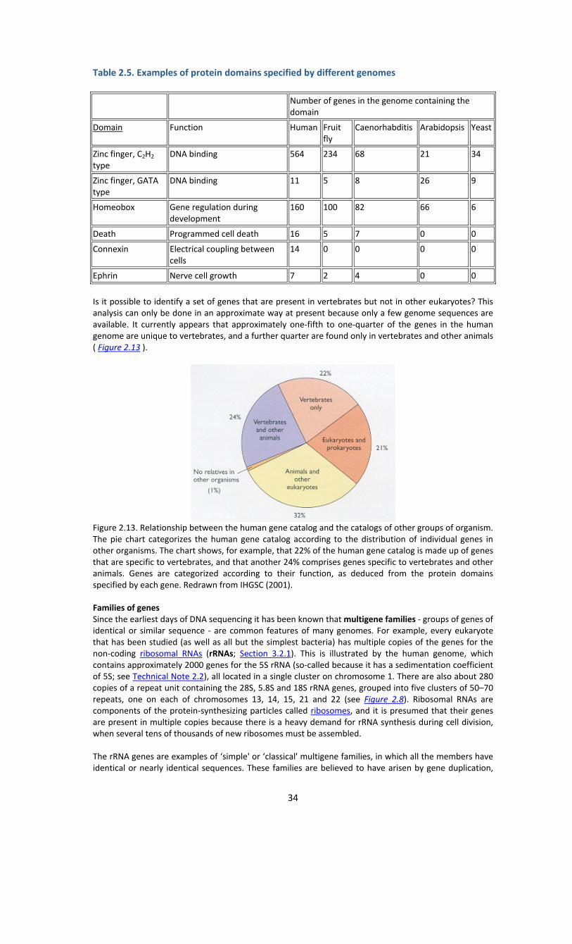
2.3. The Anatomy of the Prokaryotic Genome Because of the relatively small sizes of prokaryotic genomes, many complete genome sequences for various bacteria and archaea have been published over the last few years. As a result, we are beginning to understand a great deal about the anatomies of prokaryotic genomes, and in many respects we know more about these organisms than we do about eukaryotes. 2.3.1. The physical structure of the prokaryotic genome Most prokaryotic genomes are less than 5 Mb in size, although a few are substantially larger than this: B. megaterium, for example, has a huge genome of 30 Mb. The traditional view has been that in a typical prokaryote the genome is contained in a single circular DNA molecule, localized within the nucleoid ‐ the lightly staining region of the otherwise featureless prokaryotic cell (see Figure 2.1). This is certainly true for E. coli and many of the other commonly studied bacteria. However, as we will see, our growing knowledge of prokaryotic genomes is leading us to question several of the preconceptions that became established during the pre‐genome era of microbiology. These preconceptions relate both to the physical structure of the prokaryotic genome and its genetic organization. The traditional view of the bacterial ‘chromosome' As with eukaryotic chromosomes, a prokaryotic genome has to squeeze into a relatively tiny space (the circular E. coli chromosome has a circumference of 1.6 mm whereas an E. coli cell is just 1.0 × 2.0 μm) and, as with eukaryotes, this is achieved with the help of DNA‐binding proteins that package the genome in an organized fashion. The resulting structure has no substantial similarities with a eukaryotic chromosome, but we still use ‘bacterial chromosome' as a convenient term to describe it. Most of what we know about the organization of DNA in the nucleoid comes from studies of E. coli. The first feature to be recognized was that the circular E. coli genome is supercoiled. Supercoiling occurs when additional turns are introduced into the DNA double helix (positive supercoiling) or if turns are removed (negative supercoiling). With a linear molecule, the torsional stress introduced by over‐ or under‐winding is immediately released by rotation of the ends of the DNA molecule, but a circular molecule, having no ends, cannot reduce the strain in this way. Instead the circular molecule responds by winding around itself to form a more compact structure ( Figure 2.17 ). Supercoiling is therefore an ideal way to package a circular molecule into a small space. Evidence that supercoiling is involved in packaging the circular E. coli genome was first obtained in the 1970s from examination of isolated nucleoids, and subsequently confirmed as a feature of DNA in living cells in 1981. In E. coli, the supercoiling is thought to be generated and controlled by two enzymes, DNA gyrase and DNA topoisomerase I, which we will look at in more detail in Section 13.1.2 when we examine the roles of these enzymes in DNA replication.

40

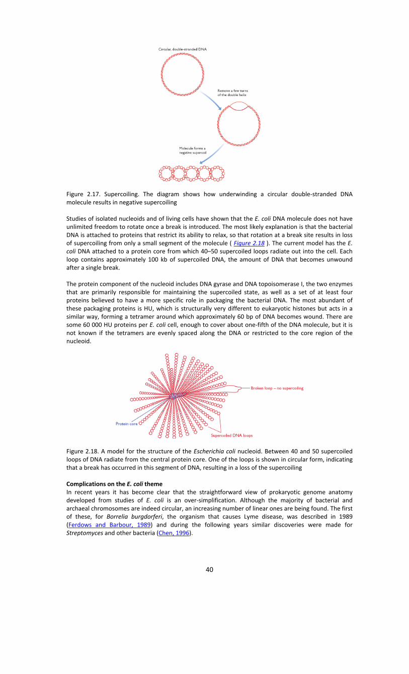
Figure 2.17. Supercoiling. The diagram shows how underwinding a circular double‐stranded DNA molecule results in negative supercoiling Studies of isolated nucleoids and of living cells have shown that the E. coli DNA molecule does not have unlimited freedom to rotate once a break is introduced. The most likely explanation is that the bacterial DNA is attached to proteins that restrict its ability to relax, so that rotation at a break site results in loss of supercoiling from only a small segment of the molecule ( Figure 2.18 ). The current model has the E. coli DNA attached to a protein core from which 40–50 supercoiled loops radiate out into the cell. Each loop contains approximately 100 kb of supercoiled DNA, the amount of DNA that becomes unwound after a single break. The protein component of the nucleoid includes DNA gyrase and DNA topoisomerase I, the two enzymes that are primarily responsible for maintaining the supercoiled state, as well as a set of at least four proteins believed to have a more specific role in packaging the bacterial DNA. The most abundant of these packaging proteins is HU, which is structurally very different to eukaryotic histones but acts in a similar way, forming a tetramer around which approximately 60 bp of DNA becomes wound. There are some 60 000 HU proteins per E. coli cell, enough to cover about one‐fifth of the DNA molecule, but it is not known if the tetramers are evenly spaced along the DNA or restricted to the core region of the nucleoid.

Figure 2.18. A model for the structure of the Escherichia coli nucleoid. Between 40 and 50 supercoiled loops of DNA radiate from the central protein core. One of the loops is shown in circular form, indicating that a break has occurred in this segment of DNA, resulting in a loss of the supercoiling Complications on the E. coli theme In recent years it has become clear that the straightforward view of prokaryotic genome anatomy developed from studies of E. coli is an over‐simplification. Although the majority of bacterial and archaeal chromosomes are indeed circular, an increasing number of linear ones are being found. The first of these, for Borrelia burgdorferi, the organism that causes Lyme disease, was described in 1989 (Ferdows and Barbour, 1989) and during the following years similar discoveries were made for Streptomyces and other bacteria (Chen, 1996).

41

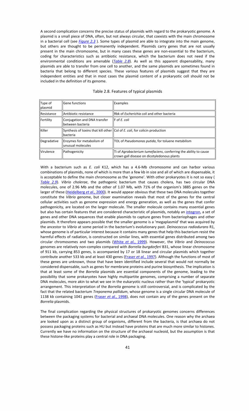
A second complication concerns the precise status of plasmids with regard to the prokaryotic genome. A plasmid is a small piece of DNA, often, but not always circular, that coexists with the main chromosome in a bacterial cell (see Figure 2.3 ). Some types of plasmid are able to integrate into the main genome, but others are thought to be permanently independent. Plasmids carry genes that are not usually present in the main chromosome, but in many cases these genes are non‐essential to the bacterium, coding for characteristics such as antibiotic resistance, which the bacterium does not need if the environmental conditions are amenable (Table 2.8). As well as this apparent dispensability, many plasmids are able to transfer from one cell to another, and the same plasmids are sometimes found in bacteria that belong to different species. These various features of plasmids suggest that they are independent entities and that in most cases the plasmid content of a prokaryotic cell should not be included in the definition of its genome.

Table 2.8. Features of typical plasmids Type of plasmid

Gene functions Examples

Resistance Antibiotic resistance Rbk of Escherichia coli and other bacteria

Fertility Conjugation and DNA transfer between bacteria

F of E. coli

Killer Synthesis of toxins that kill other bacteria

Col of E. coli, for colicin production

Degradative Enzymes for metabolism of unusual molecules

TOL of Pseudomonas putida, for toluene metabilism

Virulence Pathogenicity Ti of Agrobacterium tumefaciens, conferring the ability to cause crown gall disease on dicotyledonous plants

With a bacterium such as E. coli K12, which has a 4.6‐Mb chromosome and can harbor various combinations of plasmids, none of which is more than a few kb in size and all of which are dispensable, it is acceptable to define the main chromosome as the ‘genome'. With other prokaryotes it is not so easy ( Table 2.9). Vibrio cholerae, the pathogenic bacterium that causes cholera, has two circular DNA molecules, one of 2.96 Mb and the other of 1.07 Mb, with 71% of the organism's 3885 genes on the larger of these (Heidelberg et al., 2000). It would appear obvious that these two DNA molecules together constitute the Vibrio genome, but closer examination reveals that most of the genes for the central cellular activities such as genome expression and energy generation, as well as the genes that confer pathogenicity, are located on the larger molecule. The smaller molecule contains many essential genes but also has certain features that are considered characteristic of plasmids, notably an integron, a set of genes and other DNA sequences that enable plasmids to capture genes from bacteriophages and other plasmids. It therefore appears possible that the smaller genome is a ‘megaplasmid' that was acquired by the ancestor to Vibrio at some period in the bacterium's evolutionary past. Deinococcus radiodurans R1, whose genome is of particular interest because it contains many genes that help this bacterium resist the harmful effects of radiation, is constructed on similar lines, with essential genes distributed among two circular chromosomes and two plasmids (White et al., 1999). However, the Vibrio and Deinococcus genomes are relatively non‐complex compared with Borrelia burgdorferi B31, whose linear chromosome of 911 kb, carrying 853 genes, is accompanied by 17 or 18 linear and circular plasmids which together contribute another 533 kb and at least 430 genes (Fraser et al., 1997). Although the functions of most of these genes are unknown, those that have been identified include several that would not normally be considered dispensable, such as genes for membrane proteins and purine biosynthesis. The implication is that at least some of the Borrelia plasmids are essential components of the genome, leading to the possibility that some prokaryotes have highly multipartite genomes, comprising a number of separate DNA molecules, more akin to what we see in the eukaryotic nucleus rather than the ‘typical' prokaryotic arrangement. This interpretation of the Borrelia genome is still controversial, and is complicated by the fact that the related bacterium Treponema pallidum, whose genome is a single circular DNA molecule of 1138 kb containing 1041 genes (Fraser et al., 1998), does not contain any of the genes present on the Borrelia plasmids. The final complication regarding the physical structures of prokaryotic genomes concerns differences between the packaging systems for bacterial and archaeal DNA molecules. One reason why the archaea are looked upon as a distinct group of organisms, different from the bacteria, is that archaea do not possess packaging proteins such as HU but instead have proteins that are much more similar to histones. Currently we have no information on the structure of the archaeal nucleoid, but the assumption is that these histone‐like proteins play a central role in DNA packaging.

42

Table 2.9. Examples of genome organization in prokaryotes

Genome organization

Species DNA molecules Size (Mb) Number of genes

Escherichia coli K‐12 One circular molecule 4.639 4397

Vibrio cholerae El Tor N16961 Two circular molecules

Main chromosome 2.961 2770

Megaplasmid 1.073 1115

Deinococcus radiodurans R1 Four circular molecules

Chromosome 1 2.649 2633

Chromosome 2 0.412 369

Megaplasmid 0.177 145

Plasmid 0.046 40

Borrelia burgdorferi B31 seven or eight circular molecules, 11 linear molecules

Linear chromosome 0.911 853

Circular plasmid cp9 0.009 12

Circular plasmid cp26 0.026 29

Circular plasmid cp32* 0.032 Not known

Linear plasmid lp17 0.017 25

Linear plasmid lp25 0.024 32

Linear plasmid lp28‐1 0.027 32

Linear plasmid lp28‐2 0.030 34

Linear plasmid lp28‐3 0.029 41

Linear plasmid lp28‐4 0.027 43

Linear plasmid lp36 0.037 54

Linear plasmid lp38 0.039 52

Linear plasmid lp54 0.054 76

Linear plasmid lp56 0.056 Not known * There are 5 or 6 similar versions of plasmid cp32 per bacterium.

2.3.2. The genetic organization of the prokaryotic genome We have already learnt that bacterial genomes have compact genetic organizations with very little space between genes (see Figure 2.2 ). To re‐emphasize this point, the complete circular gene map of the E. coli K12 genome is shown in Figure 2.19 . There is non‐coding DNA in the E. coli genome, but it accounts for only 11% of the total and it is distributed around the genome in small segments that do not show up when the map is drawn at this scale. In this regard, E. coli is typical of all prokaryotes whose genomes have so far been sequenced ‐ prokaryotic genomes have very little wasted space. There are theories that this compact organization is beneficial to prokaryotes, for example by enabling the genome to be replicated relatively quickly, but these ideas have never been supported by hard experimental evidence. Operons are characteristic features of prokaryotic genomes.

Figure 2.19. The genome of Escherichia coli K12. The map is shown with the origin of replication (Section 13.2.1) positioned at the top. Genes on the outside of the circle are transcribed in the clockwise direction and those on the inside are transcribed in the anticlockwise direction. Image supplied courtesy of Dr FR Blattner, Laboratory of Genetics, University of Wisconsin‐Madison. Reproduced with permission One characteristic feature of prokaryotic genomes illustrated by E. coli is the presence of operons. In the years before genome sequences, it was thought that we understood operons very well; now we are not so sure.

43

An operon is a group of genes that are located adjacent to one another in the genome, with perhaps just one or two nucleotides between the end of one gene and the start of the next. All the genes in an operon are expressed as a single unit. This type of arrangement is common in prokaryotic genomes. A typical E. coli example is the lactose operon, the first operon to be discovered (Jacob and Monod, 1961), which contains three genes involved in conversion of the disaccharide sugar lactose into its monosaccharide units ‐ glucose and galactose (Figure 2.20A). The monosaccharides are substrates for the energy‐generating glycolytic pathway, so the function of the genes in the lactose operon is to convert lactose into a form that can be utilized by E. coli as an energy source. Lactose is not a common component of E. coli's natural environment, so most of the time the operon is not expressed and the enzymes for lactose utilization are not made by the bacterium. When lactose becomes available, it switches on the operon; all three genes are expressed together, resulting in coordinated synthesis of the lactose‐utilizing enzymes. This is the classic example of gene regulation in bacteria, and is examined in detail in Section 9.3.1.

Figure 2.20. Two operons of Escherichia coli. (A) The lactose operon. The three genes are called lacZ, lacY and lacA, the first two separated by 52 bp and the second two by 64 bp. All three genes are expressed together, lacY coding for the lactose permease which transports lactose into the cell, and lacZ and lacA coding for enzymes that split lactose into its component sugars ‐ galactose and glucose. (B) The tryptophan operon, which contains five genes coding for enzymes involved in the multistep biochemical pathway that converts chorismic acid into the amino acid tryptophan. The genes in the tryptophan operon are closer together than those in the lactose operon: trpE and trpD overlap by 1 bp, as do trpB and trpA; trpD and trpC are separated by 4 bp, and trpC and trpB by 12 bp. For more details on the regulation of these operons, see Sections 9.3.1 and 12.1.1 Altogether there are almost 600 operons in the E. coli K12 genome, each containing two or more genes, and a similar number are present in Bacillus subtilis. In most cases the genes in an operon are functionally related, coding for a set of proteins that are involved in a single biochemical activity such as utilization of a sugar as an energy source or synthesis of an amino acid. An example of the latter is the tryptophan operon of E. coli (Figure 2.20B). Microbial geneticists are attracted to the simplicity of this system whereby a bacterium is able to control its various biochemical activities by regulating the expression of groups of related genes linked together in operons. This may be a correct interpretation of the function of operons in E. coli, Bacillus subtilis and many other prokaryotes, but in at least some species the picture is less straightforward. Both the archaeon Methanococcus jannaschii and the bacterium Aquifex aeolicus have operons, but the genes in an individual operon rarely have any biochemical relationship. For example, one of the operons in the A. aeolicus genome contains six linked

44

genes, these genes coding for two proteins involved in DNA recombination (Section 14.3), an enzyme used in protein synthesis, a protein required for motility, an enzyme involved in nucleotide synthesis, and an enzyme for lipid synthesis (Figure 2.21 ; Deckert et al., 1998). This is typical of the operon structure in the A. aeolicus and M. jannaschii genomes. In other words, the notion that expression of an operon leads to the coordinated synthesis of enzymes required for a single biochemical pathway does not hold for these species.

Figure 2.21. A typical operon in the genome of Aquifex aeolicus. The genes code for the following proteins: gatC, glutamyl‐tRNA aminotransferase subunit C, which plays a role in protein synthesis (Section 11.2); recA, recombination protein RecA; pilU, twitching mobility protein; cmk, cytidylate kinase, required for synthesis of cytidine nucleotides; pgsA, phosphotidylglycerophosphate synthase, an enzyme involved in lipid biosynthesis; recJ, single‐strand‐specific endonuclease RecJ, which is another recombination protein (Section 14.3). Genome projects have therefore confused our understanding of operons. It is certainly too early to abandon the belief that operons play a central role in biochemical regulation in many bacteria, but we need to explain the unexpected features of the operons in A. aeolicus and M. jannaschii. It has been pointed out that both A. aeolicus and M. jannaschii are autotrophs, which means that, unlike many prokaryotes, they are able to synthesize organic compounds from carbon dioxide (Deckert et al., 1998), but how this similarity between the species might be used to explain their operon structures is not clear. Prokaryotic genomes and the species concept Genome projects have also confused our understanding of what constitutes a ‘species' in the prokaryotic world. This has always been a problem in microbiology because the standard biological definitions of species have been difficult to apply to microorganisms. The early taxonomists such as Linneaus described species in morphological terms, all members of one species having the same or very similar structural features. This form of classification was in vogue until the early 20th century and was first applied to microorganisms in the 1880s by Robert Koch and others, who used staining and biochemical tests to distinguish between bacterial species. However, it was recognized that this type of classification was imprecise because many of the resulting species were made up of a variety of types with quite different properties. An example is provided by E. coli which, like many bacterial species, includes strains with distinctive pathogenic characteristics, ranging from harmless through to lethal. During the 20th century, biologists redefined the species concept in evolutionary terms and we now look on a species as a group of organisms that can interbreed with one another. If anything, this is more problematic with microorganisms because there are a variety of methods by which genes can be exchanged between prokaryotes that, according to their biochemical and physiological properties, are different species (Box 2.3). The barrier to gene flow that is central to the species concept therefore does not hold with prokaryotes. Genome sequencing has emphasized the difficulties in applying the species concept to prokaryotes. It has become clear that different strains of a single species can have very different genome sequences, and may even have individual sets of strain‐specific genes. This was first shown by a comparison between two strains of Helicobacter pylori, which causes gastric ulcers and other diseases of the human digestive tract. The two strains were isolated in the UK and USA and have genomes of 1.67 Mb and 1.64 Mb, respectively. The larger genome contains 1552 genes and the smaller one 1495 genes, 1406 of these genes being present in both strains. In other words, some 6–7% of the gene content of each strain is unique to that strain (Alm et al., 1999). A much more extreme distinction between strains was revealed when the sequence of the common laboratory strain of E. coli, K12, was compared with that of one of the most pathogenic strains, O157:H7 (Perna et al., 2001). The lengths of the two genomes are significantly different ‐ 4.64 Mb for K12 and 5.53 Mb for O157:H7 ‐ with the extra DNA in the pathogenic strain scattered around the genome at almost 200 separate positions. These ‘O‐islands' contain 1387 genes not present in E. coli K12, many of these genes coding for toxins and other proteins that are clearly involved in the pathogenic properties of O157:H7. But it is not simply a case of O157:H7 containing extra genes that make it pathogenic. K12 also has 234 segments of its own unique DNA, and although these ‘K‐islands' are, on average, smaller than the O‐islands, they still contain 528 genes that are absent from O157:H7. The situation therefore is that E. coli O157:H7 and E. coli K12 each has a set of strain‐specific genes, which make up 26% and 12% of the gene catalogs, respectively. This is substantially more variation than can be tolerated by the species concept as applied to higher organisms, and is difficult to reconcile with any definition of species yet devised for microorganisms.

45

The difficulties become even more acute when other bacterial and archaeal genomes are examined. Because of the ease with which genes can flow between different prokaryotic species (Box 2.3), it was anticipated that the same genes would occasionally be found in different species, but the extent of lateral gene transfer revealed by sequencing has taken everybody by surprise (Ochman et al., 2000). Most genomes contain a few hundred kb of DNA acquired directly from a different species, and in some cases the figure is higher: 12.8% of the E. coli K12 genome, corresponding to 0.59 Mb, has been obtained in this way (Figure 2.22). A second surprise is that transfer has occurred between very different species, even between bacteria and archaea. For example, the thermophilic bacterium Thermatoga maritima has 1877 genes, 451 of which appear to have been obtained from archaeons (Nelson et al., 1999). Transfer in the other direction, from bacteria to archaea, is equally prevalent. The picture that is emerging is one in which prokaryotes living in similar ecological niches exchange genes with one another in order to increase their individual fitness for survival in their particular environment. Many of the Thermatoga genes that have been obtained from archaeons have probably helped this bacterium acquire its ability to tolerate high temperatures.

Figure 2.22. The impact of lateral gene transfer on the content of prokaryotic genomes. The chart shows the DNA that is unique to a particular species in blue and the DNA that has been acquired by lateral gene transfer in red. The number at the end of each bar indicates the percentage of the genome that derives from lateral transfer. Note that intergenic regions are omitted from this analysis. Redrawn from Ochman et al. (2000) Lateral gene transfer has clearly played an important role in the evolution of prokaryotes. Unlike higher organisms, the evolutionary histories of bacteria and archaea cannot be described as a simple branching pattern, but instead have to incorporate the horizontal flow of genes between species (Figure 2.23). As well as its impact on our understanding of evolution, lateral gene transfer also has implications for the way in which evolutionary relationships are inferred by molecular phylogenetics (Chapter 16). With higher organisms, comparisons between the sequences of equivalent genes in different species can be used to reconstruct the evolutionary relationships between those species. This type of analysis assumes that evolution has followed the simple branching pattern illustrated in Figure 2.23A , and cannot, therefore, be used to infer relationships between prokaryotes if there is a chance that the genes being analyzed have been transferred laterally between any of the species being studied. But the analysis was used for many years before the extent of lateral gene transfer was recognized and microbiologists are now faced with the need to reassess the validity of the evolutionary schemes that were established in the pre‐genome era (Doolittle, 1999).

46

Figure 2.23. Lateral gene transfer obscures the evolutionary relationships between species. In (A) a group of eight modern species has evolved from an ancestor without lateral gene transfer. The evolutionary relationships between the species can be inferred by comparisons between their DNA sequences, using the molecular phylogenetics techniques described in Chapter 16. In (B) extensive lateral gene transfer has occurred. The evolutionary histories of the modern species cannot now be inferred by standard molecular phylogenetics because one or more of the species may have acquired the sequences that are being compared by lateral gene transfer rather than by inheritance from a direct ancestor Speculation on the minimal genome content and the identity of distinctiveness genes Even though a number of prokaryotic genome sequences have now been published, it is not yet possible to describe a complete catalog of the gene content of any one species, for the simple reason that the functions of many of the genes are unknown. Over 1500 of the E. coli K12 genes, for example, have not yet been assigned a function. Despite the incompleteness of the information, it is still interesting to examine the roles of the genes whose functions are known, and to appreciate the number of different genes involved in each of the various biochemical activities that a bacterium such as E. coli is able to carry out (Table 2.10). Gene catalogs are even more interesting when comparisons are made between different species. We see, for example, that whereas 243 of the identified genes in the E. coli genome are involved in energy metabolism, Haemophilus influenzae has only 112 genes in this category and Mycoplasma genitalium just 31. These comparisons have led to speculation about the smallest number of genes needed to specify a free‐living cell. Theoretical considerations initially led to the suggestion that 256 genes are the minimum required (Mushegian and Koonin, 1996), but experiments in which increasing numbers of Mycoplasma genes have been mutated suggest that 265–350 are needed (Hutchison et al., 1999). There has been similar interest in searching for ‘distinctiveness' genes ‐ ones that distinguish one species from another. Of the 470 genes in the M. genitalium genome, 350 are also present in the distantly related bacterium Bacillus subtilis (Doolittle, 1997), which suggests that the biochemical and structural features that distinguish a Mycoplasma from a Bacillus are encoded in the 120 or so genes that are unique to the former. Unfortunately, the identities of these supposed distinctiveness genes do not provide any obvious clues about what makes a bacterium a Mycoplasma rather than anything else.

47

Table 2.10. Partial gene catalogs for Escherichia coli K12, Haeomphilus influenzae Rd and Mycoplasma genitalium

Number of genes in

Category E. coli K12 H. influenzae Rd M. genitalium

Total protein‐coding genes 4288 1727 470

Biosynthesis of amino acids 131 68 1

Biosynthesis of cofactors 103 54 5

Biosynthesis of nucleotides 58 53 19

Cell envelope proteins 237 84 17

Energy metabolism 243 112 31

Intermediary metabolism 188 30 6

Lipid metabolism 48 25 6

DNA replication, recombination and repair 115 87 32

Protein folding 9 6 7

Regulatory proteins 178 64 7

Transcription 55 27 12

Translation 182 141 101

Uptake of molecules from the environment

427 123 34

Taken from Fraser et al. (1995) and Blattner et al. (1997). The numbers refer only to genes whose functions are known and are therefore approximate, because each genome also contains many genes whose functions have not yet been identified.

2.4. The Repetitive DNA Content of Genomes Repetitive DNA is the one aspect of genome structure that we have not examined in detail. Figure 2.2 (page 34) showed us that repetitive DNA is found in all organisms and that in some, including humans, it makes up a substantial fraction of the entire genome. There are various types of repetitive DNA, and several classification systems have been devised. The scheme that we will use begins by dividing the repeats into those that are clustered into tandem arrays and those that are dispersed around the genome. 2.4.1. Tandemly repeated DNA Tandemly repeated DNA is a common feature of eukaryotic genomes but is found much less frequently in prokaryotes. This type of repeat is also called satellite DNA because DNA fragments containing tandemly repeated sequences form ‘satellite' bands when genomic DNA is fractionated by density gradient centrifugation (see Technical Note 2.2). For example, when broken into fragments 50–100 kb in length, human DNA forms a main band (buoyant density 1.701 g cm‐3) and three satellite bands (1.687, 1.693 and 1.697 g cm‐3). The main band contains DNA fragments made up mostly of single‐copy sequences with GC compositions close to 40.3%, the average value for the human genome. The satellite bands contain fragments of repetitive DNA, and hence have GC contents and buoyant densities that are atypical of the genome as a whole ( Figure 2.24 ). Satellite DNA is found at centromeres and elsewhere in eukaryotic chromosomes The satellite bands in density gradients of eukaryotic DNA are made up of fragments composed of long series of tandem repeats, possibly hundreds of kb in length. A single genome can contain several different types of satellite DNA, each with a different repeat unit, these units being anything from < 5 to > 200 bp. The three satellite bands in human DNA include at least four different repeat types. We have already encountered one type of human satellite DNA, the alphoid DNA repeats found in the centromere regions of chromosomes (see page 38). Although some satellite DNA is scattered around the genome, most is located in the centromeres, where it may play a structural role, possibly as binding sites

48

for one or more of the special centromeric proteins (see page 39). Alternatively, the repetitive DNA content of the centromere might be a reflection of the fact that this is the last region of the chromosome to be replicated. In order to delay its replication until the very end of the cell cycle, the centromere DNA must lack sequences that can act as origins of replication. The repetitive nature of centromeric DNA may be a means of ensuring that such origins are absent (Csink and Henikoff, 1998).

Figure 2.24. Satellite DNA from the human genome. Human DNA has an average GC content of 40.3% and average buoyant density of 1.701 g cm‐3. Fragments made up mainly of single‐copy DNA have a GC content close to this average and are contained in the main band in the density gradient. The satellite bands at 1.687, 1.693 and 1.697 g cm‐3 consist of fragments containing repetitive DNA. The GC contents of these fragments depend on their repeat motif sequences and are different from the genome average, meaning that these fragments have different buoyant densities to single‐copy DNA and migrate to different positions in the density gradient. Minisatellites and microsatellites Although not appearing in satellite bands on density gradients, two other types of tandemly repeated DNA are also classed as ‘satellite' DNA. These are minisatellites and microsatellites. Minisatellites form clusters up to 20 kb in length, with repeat units up to 25 bp; microsatellite clusters are shorter, usually < 150 bp, and the repeat unit is usually 13 bp or less. Minisatellite DNA is a second type of repetitive DNA that we are already familiar with because of its association with structural features of chromosomes. Telomeric DNA, which in humans comprises hundreds of copies of the motif 5′‐TTAGGG‐3′ (see Figure 2.10 ), is an example of a minisatellite. We know a certain amount about how telomeric DNA is formed, and we know that it has an important function in DNA replication (Section 13.2.4). In addition to telomeric minisatellites, some eukaryotic genomes contain various other clusters of minisatellite DNA, many, although not all, near the ends of chromosomes. The functions of these other minisatellite sequences have not been identified. The function of microsatellites is equally mysterious. The typical microsatellite consists of a 1‐, 2‐, 3‐ or 4‐bp unit repeated 10–20 times, as illustrated by the microsatellites in the human β T‐cell receptor locus (Section 1.2.1). Although each microsatellite is relatively short, there are many of them in the genome (see Table 1.3 ). In humans, for example, microsatellites with a CA repeat, such as:

make up 0.25% of the genome, 8 Mb in all. Single base‐pair repeats such as:

make up another 0.15%. Although their function, if any, is unknown, microsatellites have proved very useful to geneticists. Many microsatellites are variable, meaning that the number of repeat units in the array is different in different members of a species. This is because ‘slippage' sometimes occurs when a microsatellite is copied during DNA replication, leading to insertion or, less frequently, deletion of one or more of the repeat units (see Figure 14.5 ). No two humans alive today have exactly the same combination of microsatellite length variants: if enough microsatellites are examined then a unique genetic profile can be established for every person. The only exceptions are genetically identical twins. Genetic profiling is well known as a tool in forensic science (Figure 2.25), but identification of criminals is a fairly trivial application of microsatellite variability. More sophisticated methodology makes use of the fact that a person's genetic profile is inherited partly from the mother and partly from the father. This means that microsatellites can be used to establish kinship relationships and population affinities, not only for humans but also for other animals, and for plants.

49

Figure 2.25. The use of microsatellite analysis in genetic profiling. In this example, microsatellites located on the short arm of chromosome 6 have been amplified by the polymerase chain reaction (PCR; Section 4.3). The PCR products are labeled with a blue or green fluorescent marker and run in a polyacrylamide gel (see Technical Note 6.1), each lane showing the genetic profile of a different individual. No two individuals have the same genetic profile because each person has a different set of microsatellite length variants, the variants giving rise to bands of different sizes after PCR. The red bands are DNA size markers. Image supplied courtesy of PE Biosystems, Warrington, UK, and reproduced with permission. 2.4.2. Interspersed genome‐wide repeats Tandemly repeated DNA sequences are thought to have arisen by expansion of a progenitor sequence, either by replication slippage, as described for microsatellites, or by DNA recombination processes (Section 14.3). Both of these events are likely to result in a series of linked repeats, rather than individual repeat units scattered around the genome. Interspersed repeats must therefore have arisen by a different mechanism, one that can result in a copy of a repeat unit appearing in the genome at a position distant from the location of the original sequence. The most frequent way in which this occurs is by transposition, and most interspersed repeats have inherent transpositional activity. Transposition via an RNA intermediate The precise mechanics of transposition need not worry us until we deal with recombination and related rearrangements to the genome in Section 14.3. All that we need to know at this point is that there are two alternative modes of transposition, one that involves an RNA intermediate and one that does not. The version that involves an RNA intermediate is called retrotransposition. The basic mechanism involves three steps ( Figure 2.26 ): 1. An RNA copy of the transposon is synthesized by the normal process of transcription. 2. The RNA transcript is copied into DNA, which initially exists as an independent molecule outside of

the genome. This conversion of RNA to DNA, the reverse of the normal transcription process, requires a special enzyme called reverse transcriptase. Often the reverse transcriptase is coded by a gene within the transposon and is translated from the RNA copy synthesized in step 1.

3. The DNA copy of the transposon integrates into the genome, possibly back into the same chromosome occupied by the original unit, or possibly into a different chromosome. The end result is that there are now two copies of the transposon, at different points in the genome.

Figure 2.26. Retrotransposition. Compare with Figure 1.19 (page 22), and note that the events are essentially the same as those that result in a processed pseudogene.

50

RNA transposons or retroelements are features of eukaryotic genomes but have not so far been discovered in prokaryotes. They have attracted a great deal of attention because there are clear similarities between some types of retroelement and the free‐living viruses called retroviruses, which include both benign forms and also virulent types such as the human immunodeficiency viruses that cause AIDS. These structural relationships are illustrated in Figure 2.27 and can be summarized as follows: • Retroviruses are viruses whose genomes are made of RNA and have the genetic organization

shown in Figure 2.27A . They infect many types of vertebrate. Once inside a cell, the RNA genome is copied into DNA by the reverse transcriptase specified by the viral pol gene, and the DNA copy integrates into the host genome. New viruses can be produced by copying the integrated DNA into RNA and packaging this into virus coat proteins, the latter coded by the env genes on the virus genome.

• Endogenous retroviruses (ERVs) are retroviral genomes integrated into vertebrate chromosomes. Some are still active and might, at some stage in a cell's lifetime, direct synthesis of exogenous viruses, but most are decayed relics that no longer have the capacity to form viruses (Patience et al., 1997). These inactive sequences are genome‐wide repeats but they are not capable of additional proliferation.

• Retrotransposons have sequences similar to ERVs but are features of non‐vertebrate eukaryotic genomes (i.e. plants, fungi, invertebrates and microbial eukaryotes) rather than vertebrates. Retrotransposons have very high copy numbers in some genomes, with many different types present. Most of the genome‐wide repeats in maize are retrotransposons and in this plant these elements probably make up almost half the genome (see Figure 2.2 ). There are two types of retrotransposon: the Ty3/gypsy family (Ty3 and gypsy are examples of this class in yeast and fruit fly, respectively), whose members possess the same set of genes as an ERV, and the Ty1/copia family, members of which lack the env gene ( Figure 2.27B ). Both types are able to transpose (via the mechanism depicted in Figure 2.26 ) but the absence of the env gene means that the Ty1/copia group cannot form infectious virus particles. In fact, despite the presence of env in the Ty3/gypsy genome, it has only recently been recognized that some of these elements can form viruses and hence should be looked upon as non‐vertebrate retroviruses (Song et al., 1994; Peterson‐Burch et al., 2000). Although technically they are interspersed elements, retrotransposons are sometimes found in clusters in a genome sequence as a result of the presence of preferred integration sites for transposing elements.

The three types of retroelement described so far are LTR elements, as they have long terminal repeats at either end which play a role in the transposition process (see Figure 2.27 ). Other retroelements do not have LTRs. These are called retroposons and in mammals include the following: • LINEs (long interspersed nuclear elements) contain a reverse‐transcriptase‐like gene probably

involved in the retrotransposition process ( Figure 2.27C ). An example is the human element LINE‐1, which is 6.1 kb and has a copy number of 516 000 in the human genome (see Table 1.2 ).

• SINEs (short interspersed nuclear elements) do not have a reverse transcriptase gene but can still transpose, probably by ‘borrowing' reverse transcriptase enzymes that have been synthesized by other retroelements ( Figure 2.27D ). The commonest SINE in the human genome is Alu, which has a copy number of over 1 million ( Table 1.2 ). Alu seems to be derived from the gene for the 7SL RNA, a non‐coding RNA involved in movement of proteins around the cell. The first Alu element may have arisen by the accidental reverse transcription of a 7SL RNA molecule and integration of the DNA copy into the human genome. Some Alu elements are actively copied into RNA, providing the opportunity for proliferation of the element.

Figure 2.27. Retroelements. A comparison of the structures of four types of retroelement. Retroviruses and retrotransposons are LTR elements that possess long terminal repeats at each end. The gag gene codes for a series of proteins located in the virus core; pol codes for the reverse transcriptase and other enzymes involved in replication of the element; env codes for coat proteins. LINEs and SINEs are non‐LTR retroelements or retroposons. Both have a poly(A) region (a long series of A nucleotides) at one end.

51

DNA transposons Not all transposons require an RNA intermediate. Many are able to transpose in a more direct DNA to DNA manner. With these elements we are aware of two distinct transposition mechanisms ( Figure 2.28 ), one involving direct interaction between the donor transposon and the target site, resulting in copying of the donor element (replicative transposition), and the second involving excision of the element and re‐integration at a new site (conservative transposition). Both mechanisms require enzymes which are usually coded by genes within the transposon. The molecular events that occur during these two types of transposition are described in Section 14.3.3. In eukaryotes, DNA transposons are less common than retrotransposons (see Table 1.2 ), but they have a special place in genetics because a family of plant DNA transposons ‐ the Ac/Ds elements of maize ‐ were the first transposable elements to be discovered, by Barbara McClintock in the 1950s. Her conclusions ‐ that some genes are mobile and can move from one position to another in a chromosome ‐ were based on exquisite genetic experiments, the molecular basis of transposition not being understood until the late 1970s. DNA transposons are a much more important component of prokaryotic genome anatomies than the RNA transposons. The insertion sequences, IS1 and IS186, present in the 50‐kb segment of E. coli DNA that we examined in Section 2.1.2 (see Figure 2.2 ), are examples of DNA transposons, and a single E. coli genome may contain as many as 20 of these of various types. Most of the sequence of an IS is taken up by one or two genes that specify the transposase enzyme that catalyzes its transposition ( Figure 2.29A ). IS elements can transpose either replicatively or conservatively. Other kinds of DNA transposon known in E. coli, and fairly typical of prokaryotes in general, are as follows: • Composite transposons are basically a pair of IS elements flanking a segment of DNA, usually

containing one or more genes, often ones coding for antibiotic resistance (Figure 2.29B). The transposition of a composite transposon is catalyzed by the transposase coded by one or both of the IS elements. Composite transposons use the conservative mechanism of transposition.

• Tn3‐type transposons have their own transposase gene and so do not require flanking IS elements in order to transpose ( Figure 2.29C ). Tn3 elements transpose replicatively.

• Transposable phages are bacterial viruses which transpose replicatively as part of their normal infection cycle ( Figure 2.29D ).

Figure 2.28. Two mechanisms of transposition used by DNA transposons. For more details see Section 14.3.3

Figure 2.29. DNA transposons of prokaryotes. Four types are shown. Insertion sequences, Tn3‐type transposons and transposable phages are flanked by short (< 50 bp) inverted terminal repeat (ITR) sequences. The resolvase gene of the Tn3‐type transposon codes for a protein involved in the transposition process.