CHAPTER 18: EQUITY VALUATION MODELSfaculty.bus.olemiss.edu/bvanness/fall 2008/FIN 533/End of...
17
Chapter 18 - Equity Valuation Models 18-1 CHAPTER 18: EQUITY VALUATION MODELS PROBLEM SETS 1. Theoretically, dividend discount models can be used to value the stock of rapidly growing companies that do not currently pay dividends; in this scenario, we would be valuing expected dividends in the relatively more distant future. However, as a practical matter, such estimates of payments to be made in the more distant future are notoriously inaccurate, rendering dividend discount models problematic for valuation of such companies; free cash flow models are more likely to be appropriate. At the other extreme, one would be more likely to choose a dividend discount model to value a mature firm paying a relatively stable dividend. 2. It is most important to use multi-stage dividend discount models when valuing companies with temporarily high growth rates. These companies tend to be companies in the early phases of their life cycles, when they have numerous opportunities for reinvestment, resulting in relatively rapid growth and relatively low dividends (or, in many cases, no dividends at all). As these firms mature, attractive investment opportunities are less numerous so that growth rates slow. 3. The intrinsic value of a share of stock is the individual investor’s assessment of the true worth of the stock. The market capitalization rate is the market consensus for the required rate of return for the stock. If the intrinsic value of the stock is equal to its price, then the market capitalization rate is equal to the expected rate of return. On the other hand, if the individual investor believes the stock is underpriced (i.e., intrinsic value < price), then that investor’s expected rate of return is greater than the market capitalization rate. 4. a. k = D 1 /P 0 + g 0.16 = $2/$50 + g g = 0.12 = 12% b. P 0 = D 1 /(k – g) = $2/(0.16 – 0.05) = $18.18 The price falls in response to the more pessimistic dividend forecast. The forecast for current year earnings, however, is unchanged. Therefore, the P/E ratio falls. The lower P/E ratio is evidence of the diminished optimism concerning the firm's growth prospects.
Transcript of CHAPTER 18: EQUITY VALUATION MODELSfaculty.bus.olemiss.edu/bvanness/fall 2008/FIN 533/End of...
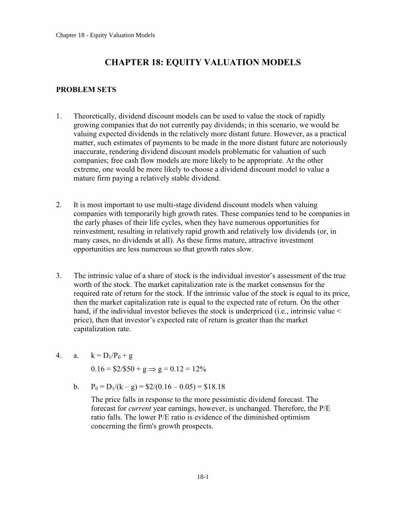
Chapter 18 - Equity Valuation Models
18-1
CHAPTER 18: EQUITY VALUATION MODELS
PROBLEM SETS
1. Theoretically, dividend discount models can be used to value the stock of rapidly
growing companies that do not currently pay dividends; in this scenario, we would be
valuing expected dividends in the relatively more distant future. However, as a practical
matter, such estimates of payments to be made in the more distant future are notoriously
inaccurate, rendering dividend discount models problematic for valuation of such
companies; free cash flow models are more likely to be appropriate. At the other
extreme, one would be more likely to choose a dividend discount model to value a
mature firm paying a relatively stable dividend.
2. It is most important to use multi-stage dividend discount models when valuing
companies with temporarily high growth rates. These companies tend to be companies in
the early phases of their life cycles, when they have numerous opportunities for
reinvestment, resulting in relatively rapid growth and relatively low dividends (or, in
many cases, no dividends at all). As these firms mature, attractive investment
opportunities are less numerous so that growth rates slow.
3. The intrinsic value of a share of stock is the individual investor’s assessment of the true
worth of the stock. The market capitalization rate is the market consensus for the
required rate of return for the stock. If the intrinsic value of the stock is equal to its price,
then the market capitalization rate is equal to the expected rate of return. On the other
hand, if the individual investor believes the stock is underpriced (i.e., intrinsic value <
price), then that investor’s expected rate of return is greater than the market
capitalization rate.
4. a. k = D1/P0 + g
0.16 = $2/$50 + g g = 0.12 = 12%
b. P0 = D1/(k – g) = $2/(0.16 – 0.05) = $18.18
The price falls in response to the more pessimistic dividend forecast. The
forecast for current year earnings, however, is unchanged. Therefore, the P/E
ratio falls. The lower P/E ratio is evidence of the diminished optimism
concerning the firm's growth prospects.
Chapter 18 - Equity Valuation Models
18-2
5. a. g = ROE b = 16% 0.5 = 8%
D1 = $2(1 – b) = $2(1 – 0.5) = $1
P0 = D1/(k – g) = $1/(0.12 – 0.08) = $25
b. P3 = P0(1 + g)3 = $25(1.08)
3 = $31.49
6. a. k = rf + (rM) – rf ] = 6% + 1.25(14% – 6%) = 16%
g = 2/3 9% = 6%
D1 = E0(1 + g) (1 – b) = $3(1.06) (1/3) = $1.06
60$10.0.060.16
$1.06
gk
DP 1
0
b. Leading P0/E1 = $10.60/$3.18 = 3.33
Trailing P0/E0 = $10.60/$3.00 = 3.53
c. 275.9$16.0
18.3$60.10$
k
EPPVGO 1
0
The low P/E ratios and negative PVGO are due to a poor ROE (9%) that is less
than the market capitalization rate (16%).
d. Now, you revise b to 1/3, g to 1/3 9% = 3%, and D1 to:
E0 1.03 (2/3) = $2.06
Thus:
V0 = $2.06/(0.16 – 0.03) = $15.85
V0 increases because the firm pays out more earnings instead of reinvesting a poor
ROE. This information is not yet known to the rest of the market.
7. Since beta = 1.0, then k = market return = 15%
Therefore:
15% = D1/P0 + g = 4% + g g = 11%
Chapter 18 - Equity Valuation Models
18-3
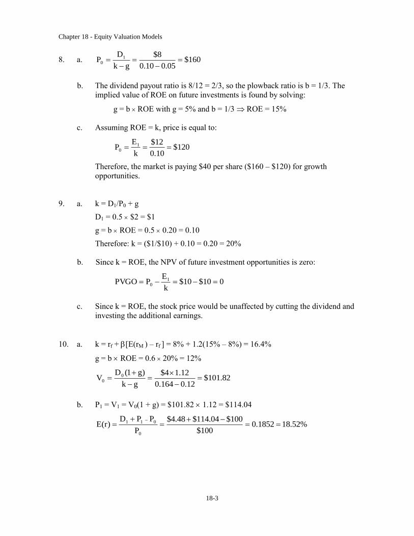
8. a. 160$05.010.0
8$
gk
DP 1
0
b. The dividend payout ratio is 8/12 = 2/3, so the plowback ratio is b = 1/3. The
implied value of ROE on future investments is found by solving:
g = b ROE with g = 5% and b = 1/3 ROE = 15%
c. Assuming ROE = k, price is equal to:
120$10.0
12$
k
EP 1
0
Therefore, the market is paying $40 per share ($160 – $120) for growth
opportunities.
9. a. k = D1/P0 + g
D1 = 0.5 $2 = $1
g = b ROE = 0.5 0.20 = 0.10
Therefore: k = ($1/$10) + 0.10 = 0.20 = 20%
b. Since k = ROE, the NPV of future investment opportunities is zero:
010$10$k
EPPVGO 1
0
c. Since k = ROE, the stock price would be unaffected by cutting the dividend and
investing the additional earnings.
10. a. k = rf +[E(rM ) – rf ] = 8% + 1.2(15% – 8%) = 16.4%
g = b ROE = 0.6 20% = 12%
82.101$12.0164.0
12.14$
gk
)g1(DV 0
0
b. P1 = V1 = V0(1 + g) = $101.82 1.12 = $114.04
%52.181852.0100$
100$04.114$48.4$
P
PPD)r(E
0
011
Chapter 18 - Equity Valuation Models
18-4
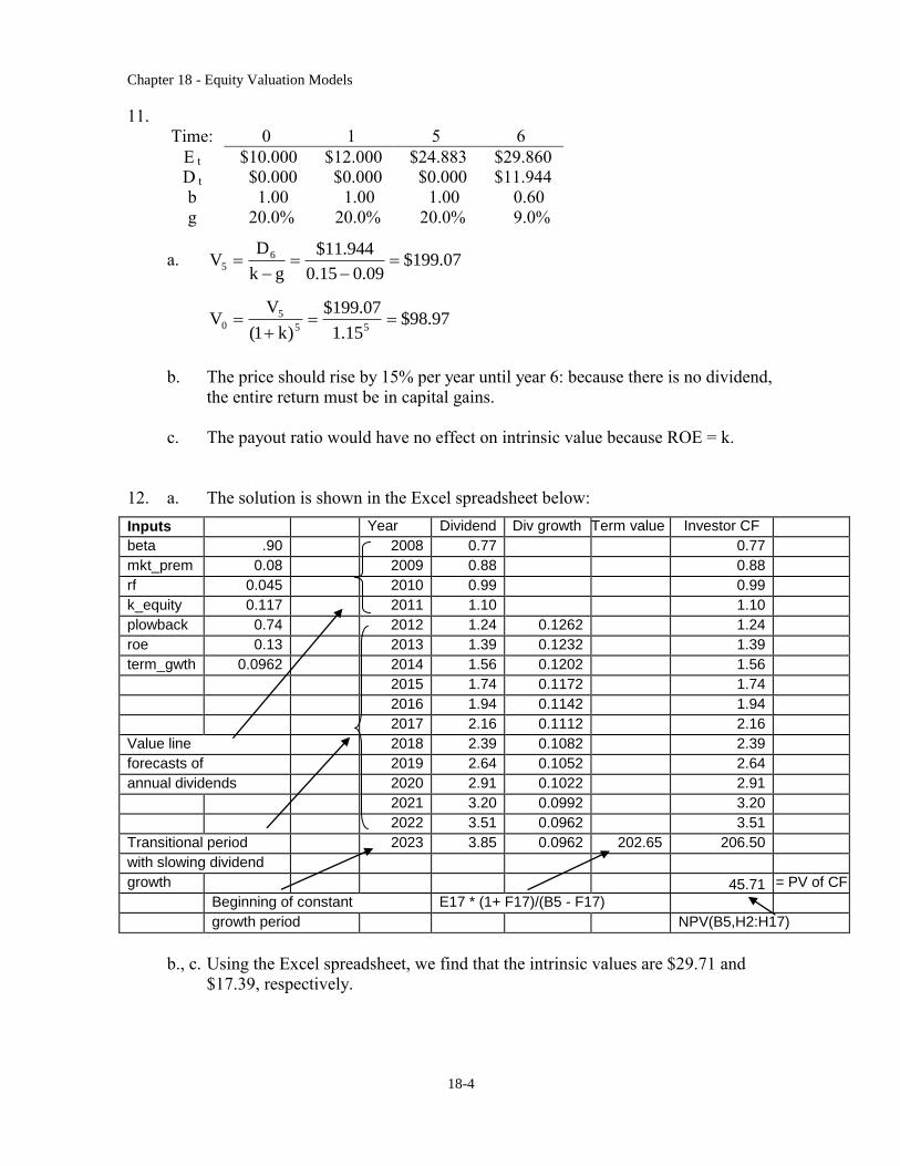
11.
Time: 0 1 5 6
E t $10.000 $12.000 $24.883 $29.860 D t $0.000 $0.000 $0.000 $11.944
b 1.00 1.00 1.00 0.60
g 20.0% 20.0% 20.0% 9.0%
a. 07.199$09.015.0
944.11$
gk
DV 6
5
97.98$15.1
07.199$
)k1(
VV
55
50
b. The price should rise by 15% per year until year 6: because there is no dividend,
the entire return must be in capital gains.
c. The payout ratio would have no effect on intrinsic value because ROE = k.
12. a. The solution is shown in the Excel spreadsheet below:
Inputs Year Dividend Div growth Term value Investor CF
beta .90
2008 0.77 0.77
mkt_prem 0.08 2009 0.88 0.88
rf 0.045 2010 0.99 0.99
k_equity 0.117 2011 1.10 1.10
plowback 0.74 2012 1.24 0.1262 1.24
roe 0.13 2013 1.39 0.1232 1.39
term_gwth 0.0962 2014 1.56 0.1202 1.56
2015 1.74 0.1172 1.74
2016 1.94 0.1142 1.94
2017 2.16 0.1112 2.16
Value line 2018 2.39 0.1082 2.39
forecasts of 2019 2.64 0.1052 2.64
annual dividends 2020 2.91 0.1022 2.91
2021 3.20 0.0992 3.20
2022 3.51 0.0962 3.51
Transitional period 2023 3.85 0.0962
202.65 206.50
with slowing dividend
growth 45.71
= PV of CF
Beginning of constant E17 * (1+ F17)/(B5 - F17)
growth period NPV(B5,H2:H17)
b., c. Using the Excel spreadsheet, we find that the intrinsic values are $29.71 and
$17.39, respectively.
Chapter 18 - Equity Valuation Models
18-5
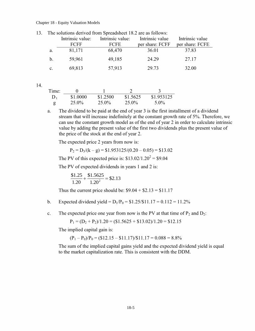
13. The solutions derived from Spreadsheet 18.2 are as follows:
Intrinsic value:
FCFF
Intrinsic value:
FCFE
Intrinsic value
per share: FCFF
Intrinsic value
per share: FCFE
a. 81,171 68,470 36.01 37.83
b. 59,961 49,185 24.29 27.17
c. 69,813 57,913 29.73 32.00
14.
Time: 0 1 2 3
D t $1.0000 $1.2500 $1.5625 $1.953125 g 25.0% 25.0% 25.0% 5.0%
a. The dividend to be paid at the end of year 3 is the first installment of a dividend
stream that will increase indefinitely at the constant growth rate of 5%. Therefore, we
can use the constant growth model as of the end of year 2 in order to calculate intrinsic
value by adding the present value of the first two dividends plus the present value of
the price of the stock at the end of year 2.
The expected price 2 years from now is:
P2 = D3/(k – g) = $1.953125/(0.20 – 0.05) = $13.02
The PV of this expected price is: $13.02/1.202 = $9.04
The PV of expected dividends in years 1 and 2 is:
13.2$20.1
5625.1$
20.1
25.1$2
Thus the current price should be: $9.04 + $2.13 = $11.17
b. Expected dividend yield = D1/P0 = $1.25/$11.17 = 0.112 = 11.2%
c. The expected price one year from now is the PV at that time of P2 and D2:
P1 = (D2 + P2)/1.20 = ($1.5625 + $13.02)/1.20 = $12.15
The implied capital gain is:
(P1 – P0)/P0 = ($12.15 – $11.17)/$11.17 = 0.088 = 8.8%
The sum of the implied capital gains yield and the expected dividend yield is equal
to the market capitalization rate. This is consistent with the DDM.
Chapter 18 - Equity Valuation Models
18-6
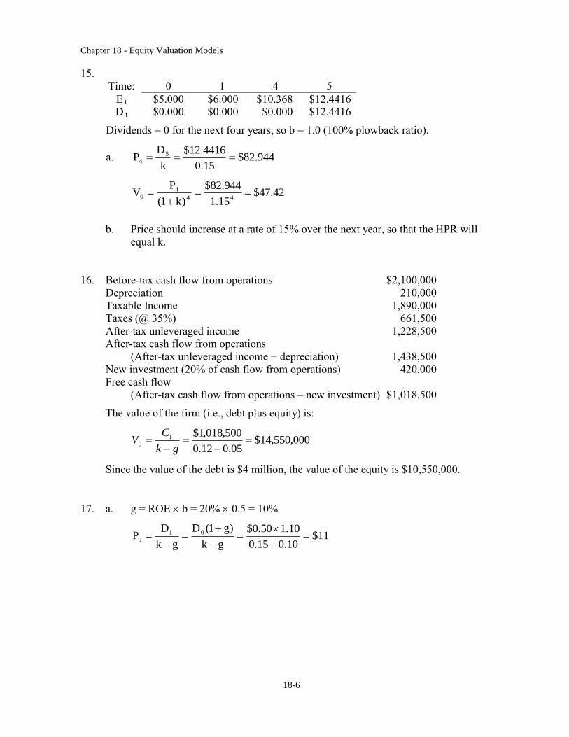
15.
Time: 0 1 4 5
E t $5.000 $6.000 $10.368 $12.4416 D t $0.000 $0.000 $0.000 $12.4416
Dividends = 0 for the next four years, so b = 1.0 (100% plowback ratio).
a. 944.82$15.0
4416.12$
k
DP 5
4
42.47$15.1
944.82$
)k1(
PV
44
40
b. Price should increase at a rate of 15% over the next year, so that the HPR will
equal k.
16. Before-tax cash flow from operations $2,100,000
Depreciation 210,000
Taxable Income 1,890,000
Taxes (@ 35%) 661,500
After-tax unleveraged income 1,228,500
After-tax cash flow from operations
(After-tax unleveraged income + depreciation) 1,438,500
New investment (20% of cash flow from operations) 420,000
Free cash flow
(After-tax cash flow from operations – new investment) $1,018,500
The value of the firm (i.e., debt plus equity) is:
000,550,14$05.012.0
500,018,1$10
gk
CV
Since the value of the debt is $4 million, the value of the equity is $10,550,000.
17. a. g = ROE b = 20% 0.5 = 10%
11$10.015.0
10.150.0$
gk
)g1(D
gk
DP 01
0
Chapter 18 - Equity Valuation Models
18-7
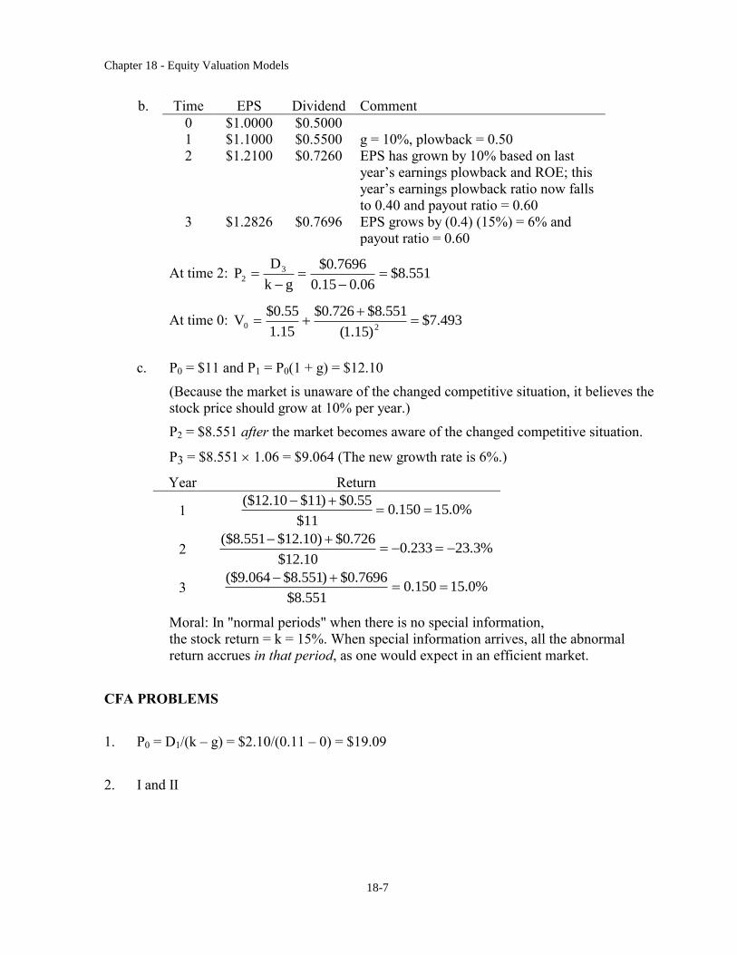
b. Time EPS Dividend Comment
0 $1.0000 $0.5000 1 $1.1000 $0.5500 g = 10%, plowback = 0.50
2 $1.2100 $0.7260 EPS has grown by 10% based on last
year’s earnings plowback and ROE; this
year’s earnings plowback ratio now falls
to 0.40 and payout ratio = 0.60
3 $1.2826 $0.7696 EPS grows by (0.4) (15%) = 6% and
payout ratio = 0.60
At time 2: 551.8$06.015.0
7696.0$
gk
DP 3
2
At time 0: 493.7$)15.1(
551.8$726.0$
15.1
55.0$V
20
c. P0 = $11 and P1 = P0(1 + g) = $12.10
(Because the market is unaware of the changed competitive situation, it believes the
stock price should grow at 10% per year.)
P2 = $8.551 after the market becomes aware of the changed competitive situation.
P3 = $8.551 1.06 = $9.064 (The new growth rate is 6%.)
Year Return
1 %0.15150.011$
55.0$)11$10.12($
2 %3.23233.010.12$
726.0$)10.12$551.8($
3 %0.15150.0551.8$
7696.0$)551.8$064.9($
Moral: In "normal periods" when there is no special information,
the stock return = k = 15%. When special information arrives, all the abnormal
return accrues in that period, as one would expect in an efficient market. CFA PROBLEMS 1. P0 = D1/(k – g) = $2.10/(0.11 – 0) = $19.09 2. I and II
Chapter 18 - Equity Valuation Models
18-8
3. a. This director is confused. In the context of the constant growth model
[i.e., P0 = D1/(k – g)], it is true that price is higher when dividends are higher
holding everything else including dividend growth constant. But everything else will
not be constant. If the firm increases the dividend payout rate, the growth rate g will
fall, and stock price will not necessarily rise. In fact, if ROE > k, price will fall.
b. (i) An increase in dividend payout will reduce the sustainable growth rate as less
funds are reinvested in the firm. The sustainable growth rate
(i.e., ROE plowback) will fall as plowback ratio falls.
(ii) The increased dividend payout rate will reduce the growth rate of book value
for the same reason -- less funds are reinvested in the firm.
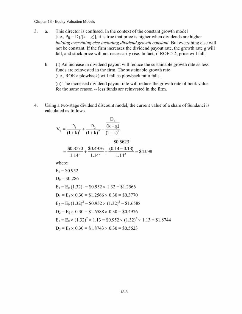
4. Using a two-stage dividend discount model, the current value of a share of Sundanci is
calculated as follows.
2
3
2
2
1
10
)k1(
)gk(
D
)k1(
D
)k1(
DV
98.43$14.1
)13.014.0(
5623.0$
14.1
4976.0$
14.1
3770.0$221
where:
E0 = $0.952
D0 = $0.286
E1 = E0 (1.32)1 = $0.952 1.32 = $1.2566
D1 = E1 0.30 = $1.2566 0.30 = $0.3770
E2 = E0 (1.32)2 = $0.952 (1.32)
2 = $1.6588
D2 = E2 0.30 = $1.6588 0.30 = $0.4976
E3 = E0 (1.32)2 1.13 = $0.952 (1.32)
3 1.13 = $1.8744
D3 = E3 0.30 = $1.8743 0.30 = $0.5623
Chapter 18 - Equity Valuation Models
18-9
5. a. Free cash flow to equity (FCFE) is defined as the cash flow remaining after
meeting all financial obligations (including debt payment) and after covering
capital expenditure and working capital needs. The FCFE is a measure of how
much the firm can afford to pay out as dividends, but in a given year may be more
or less than the amount actually paid out.
Sundanci's FCFE for the year 2008 is computed as follows:
FCFE =
Earnings after tax + Depreciation expense Capital expenditures Increase in NWC
= $80 million + $23 million $38 million $41 million = $24 million
FCFE per share = FCFE/number of shares outstanding
= $24 million/84 million shares = $0.286
At the given dividend payout ratio, Sundanci's FCFE per share equals dividends
per share.
b. The FCFE model requires forecasts of FCFE for the high growth years (2009 and
2010) plus a forecast for the first year of stable growth (2011) in order to to allow
for an estimate of the terminal value in 2010 based on perpetual growth. Because
all of the components of FCFE are expected to grow at the same rate, the values
can be obtained by projecting the FCFE at the common rate. (Alternatively, the
components of FCFE can be projected and aggregated for each year.)
The following table shows the process for estimating Sundanci's current value on a
per share basis.
Chapter 18 - Equity Valuation Models
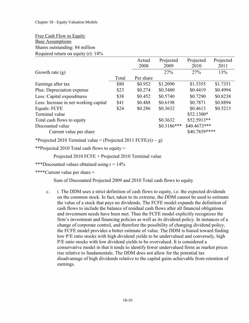
18-10
Free Cash Flow to Equity
Base Assumptions
Shares outstanding: 84 million
Required return on equity (r): 14%
Actual
2008
Projected
2009
Projected
2010
Projected
2011
Growth rate (g) 27% 27% 13%
Total Per share
Earnings after tax $80 $0.952 $1.2090 $1.5355 $1.7351
Plus: Depreciation expense $23 $0.274 $0.3480 $0.4419 $0.4994
Less: Capital expenditures $38 $0.452 $0.5740 $0.7290 $0.8238
Less: Increase in net working capital $41 $0.488 $0.6198 $0.7871 $0.8894
Equals: FCFE $24 $0.286 $0.3632 $0.4613 $0.5213
Terminal value $52.1300*
Total cash flows to equity $0.3632 $52.5913**
Discounted value $0.3186*** $40.4673***
Current value per share $40.7859****
*Projected 2010 Terminal value = (Projected 2011 FCFE)/(r g)
**Projected 2010 Total cash flows to equity =
Projected 2010 FCFE + Projected 2010 Terminal value
***Discounted values obtained using r = 14%
****Current value per share =
Sum of Discounted Projected 2009 and 2010 Total cash flows to equity
c. i. The DDM uses a strict definition of cash flows to equity, i.e. the expected dividends
on the common stock. In fact, taken to its extreme, the DDM cannot be used to estimate
the value of a stock that pays no dividends. The FCFE model expands the definition of
cash flows to include the balance of residual cash flows after all financial obligations
and investment needs have been met. Thus the FCFE model explicitly recognizes the
firm’s investment and financing policies as well as its dividend policy. In instances of a
change of corporate control, and therefore the possibility of changing dividend policy,
the FCFE model provides a better estimate of value. The DDM is biased toward finding
low P/E ratio stocks with high dividend yields to be undervalued and conversely, high
P/E ratio stocks with low dividend yields to be overvalued. It is considered a
conservative model in that it tends to identify fewer undervalued firms as market prices
rise relative to fundamentals. The DDM does not allow for the potential tax
disadvantage of high dividends relative to the capital gains achievable from retention of
earnings.
Chapter 18 - Equity Valuation Models
18-11
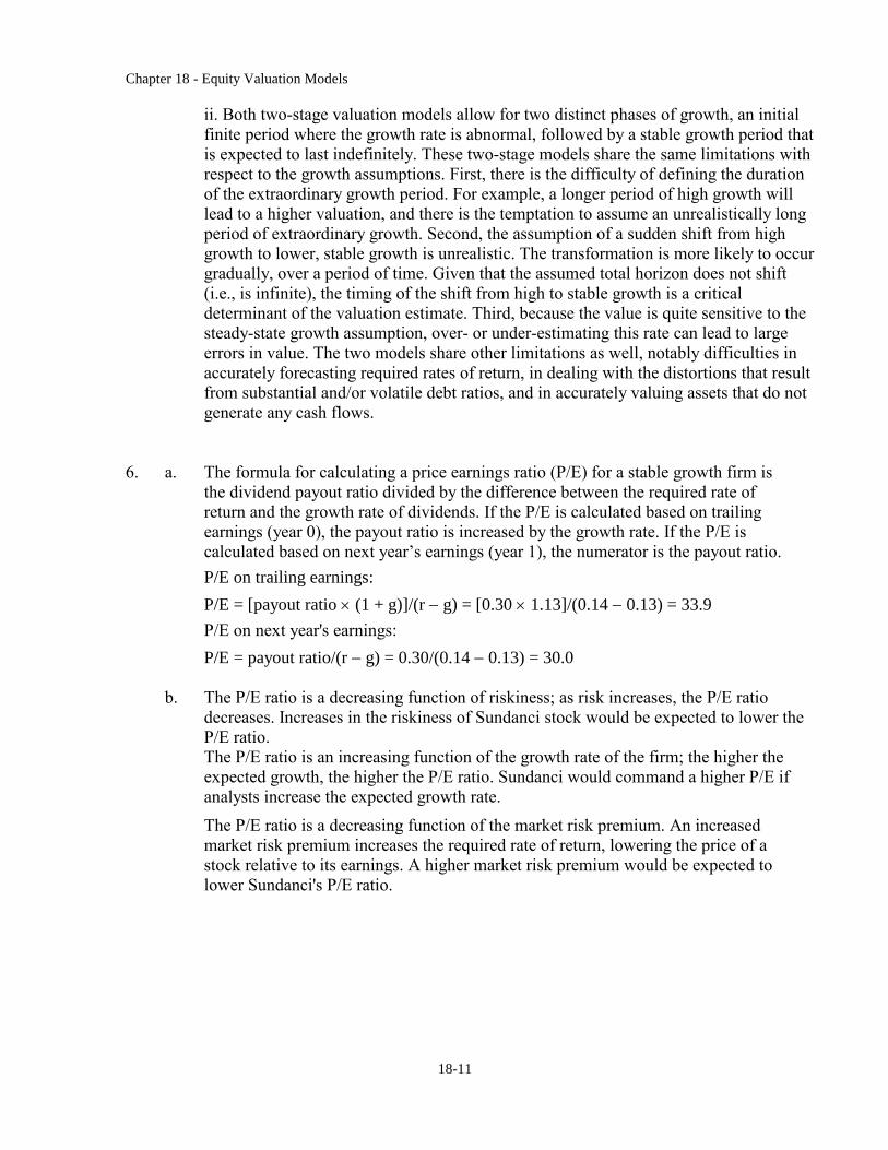
ii. Both two-stage valuation models allow for two distinct phases of growth, an initial
finite period where the growth rate is abnormal, followed by a stable growth period that
is expected to last indefinitely. These two-stage models share the same limitations with
respect to the growth assumptions. First, there is the difficulty of defining the duration
of the extraordinary growth period. For example, a longer period of high growth will
lead to a higher valuation, and there is the temptation to assume an unrealistically long
period of extraordinary growth. Second, the assumption of a sudden shift from high
growth to lower, stable growth is unrealistic. The transformation is more likely to occur
gradually, over a period of time. Given that the assumed total horizon does not shift
(i.e., is infinite), the timing of the shift from high to stable growth is a critical
determinant of the valuation estimate. Third, because the value is quite sensitive to the
steady-state growth assumption, over- or under-estimating this rate can lead to large
errors in value. The two models share other limitations as well, notably difficulties in
accurately forecasting required rates of return, in dealing with the distortions that result
from substantial and/or volatile debt ratios, and in accurately valuing assets that do not
generate any cash flows.
6. a. The formula for calculating a price earnings ratio (P/E) for a stable growth firm is
the dividend payout ratio divided by the difference between the required rate of
return and the growth rate of dividends. If the P/E is calculated based on trailing
earnings (year 0), the payout ratio is increased by the growth rate. If the P/E is
calculated based on next year’s earnings (year 1), the numerator is the payout ratio.
P/E on trailing earnings:
P/E = [payout ratio (1 + g)]/(r g) = [0.30 1.13]/(0.14 0.13) = 33.9
P/E on next year's earnings:
P/E = payout ratio/(r g) = 0.30/(0.14 0.13) = 30.0
b. The P/E ratio is a decreasing function of riskiness; as risk increases, the P/E ratio
decreases. Increases in the riskiness of Sundanci stock would be expected to lower the
P/E ratio.
The P/E ratio is an increasing function of the growth rate of the firm; the higher the
expected growth, the higher the P/E ratio. Sundanci would command a higher P/E if
analysts increase the expected growth rate.
The P/E ratio is a decreasing function of the market risk premium. An increased
market risk premium increases the required rate of return, lowering the price of a
stock relative to its earnings. A higher market risk premium would be expected to
lower Sundanci's P/E ratio.
Chapter 18 - Equity Valuation Models
18-12
7. a. The sustainable growth rate is equal to:
plowback ratio × return on equity = b × ROE
where
b = [Net Income – (Dividend per share × shares outstanding)]/Net Income
ROE = Net Income/Beginning of year equity
In 2005:
b = [208 – (0.80 × 100)]/208 = 0.6154
ROE = 208/1380 = 0.1507
Sustainable growth rate = 0.6154 × 0.1507 = 9.3%
In 2008:
b = [275 – (0.80 × 100)]/275 = 0.7091
ROE = 275/1836 = 0.1498
Sustainable growth rate = 0.7091 × 0.1498 = 10.6%
b. i. The increased retention ratio increased the sustainable growth rate.
Retention ratio = [Net Income – (Dividend per share × shares outstanding)]/Net Income
Retention ratio increased from 0.6154 in 2005 to 0.7091 in 2008. This increase in the retention ratio directly increased the sustainable growth rate
because the retention ratio is one of the two factors determining the sustainable
growth rate.
ii. The decrease in leverage reduced the sustainable growth rate.
Financial leverage = (Total Assets/Beginning of year equity)
Financial leverage decreased from 2.34 (= 3230/1380) at the beginning of 2005 to 2.10
at the beginning of 2008 (= 3856/1836)
This decrease in leverage directly decreased ROE (and thus the sustainable growth rate)
because financial leverage is one of the factors determining ROE (and ROE is one of the
two factors determining the sustainable growth rate). 8. a. The formula for the Gordon model is:
V0 = [D0 × (1 + g)]/(r – g)
where:
D0 = dividend paid at time of valuation
g = annual growth rate of dividends
r = required rate of return for equity
In the above formula, P0, the market price of the common stock, substitutes for V0
and g becomes the dividend growth rate implied by the market:
P0 = [D0 × (1 + g)]/(r – g)
Substituting, we have:
58.49 = [0.80 × (1 + g)]/(0.08 – g) g = 6.54%
Chapter 18 - Equity Valuation Models
18-13
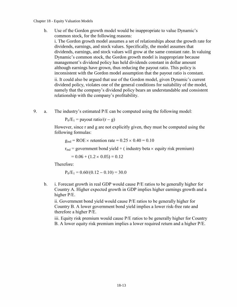
b. Use of the Gordon growth model would be inappropriate to value Dynamic’s
common stock, for the following reasons:
i. The Gordon growth model assumes a set of relationships about the growth rate for
dividends, earnings, and stock values. Specifically, the model assumes that
dividends, earnings, and stock values will grow at the same constant rate. In valuing
Dynamic’s common stock, the Gordon growth model is inappropriate because
management’s dividend policy has held dividends constant in dollar amount
although earnings have grown, thus reducing the payout ratio. This policy is
inconsistent with the Gordon model assumption that the payout ratio is constant.
ii. It could also be argued that use of the Gordon model, given Dynamic’s current
dividend policy, violates one of the general conditions for suitability of the model,
namely that the company’s dividend policy bears an understandable and consistent
relationship with the company’s profitability.
9. a. The industry’s estimated P/E can be computed using the following model:
P0/E1 = payout ratio/(r g)
However, since r and g are not explicitly given, they must be computed using the
following formulas:
gind = ROE retention rate = 0.25 0.40 = 0.10
rind = government bond yield + ( industry beta equity risk premium)
= 0.06 + (1.2 0.05) = 0.12
Therefore:
P0/E1 = 0.60/(0.12 0.10) = 30.0
b. i. Forecast growth in real GDP would cause P/E ratios to be generally higher for
Country A. Higher expected growth in GDP implies higher earnings growth and a
higher P/E.
ii. Government bond yield would cause P/E ratios to be generally higher for
Country B. A lower government bond yield implies a lower risk-free rate and
therefore a higher P/E.
iii. Equity risk premium would cause P/E ratios to be generally higher for Country
B. A lower equity risk premium implies a lower required return and a higher P/E.
Chapter 18 - Equity Valuation Models
18-14
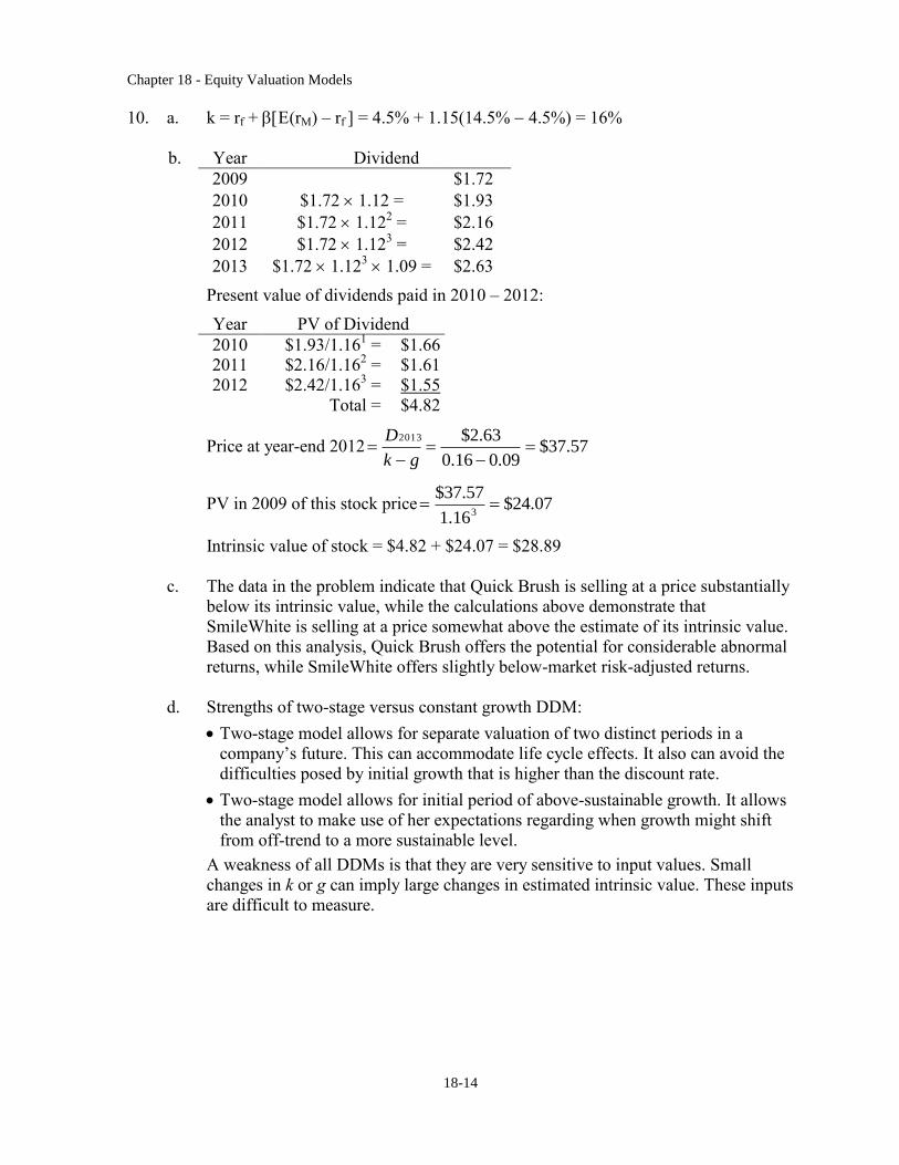
10. a. k = rf + (rM) – rf ] = 4.5% + 1.15(14.5% 4.5%) = 16%
b. Year Dividend
2009 $1.72
2010 $1.72 1.12 = $1.93
2011 $1.72 1.122 = $2.16
2012 $1.72 1.123 = $2.42
2013 $1.72 1.123 1.09 = $2.63
Present value of dividends paid in 2010 – 2012:
Year PV of Dividend
2010 $1.93/1.161 = $1.66
2011 $2.16/1.162 = $1.61
2012 $2.42/1.163 = $1.55
Total = $4.82
Price at year-end 2012 57.37$09.016.0
63.2$2013
gk
D
PV in 2009 of this stock price 07.24$16.1
57.37$3
Intrinsic value of stock = $4.82 + $24.07 = $28.89
c. The data in the problem indicate that Quick Brush is selling at a price substantially
below its intrinsic value, while the calculations above demonstrate that
SmileWhite is selling at a price somewhat above the estimate of its intrinsic value.
Based on this analysis, Quick Brush offers the potential for considerable abnormal
returns, while SmileWhite offers slightly below-market risk-adjusted returns.
d. Strengths of two-stage versus constant growth DDM:
Two-stage model allows for separate valuation of two distinct periods in a
company’s future. This can accommodate life cycle effects. It also can avoid the
difficulties posed by initial growth that is higher than the discount rate.
Two-stage model allows for initial period of above-sustainable growth. It allows
the analyst to make use of her expectations regarding when growth might shift
from off-trend to a more sustainable level.
A weakness of all DDMs is that they are very sensitive to input values. Small
changes in k or g can imply large changes in estimated intrinsic value. These inputs
are difficult to measure.
Chapter 18 - Equity Valuation Models
18-15
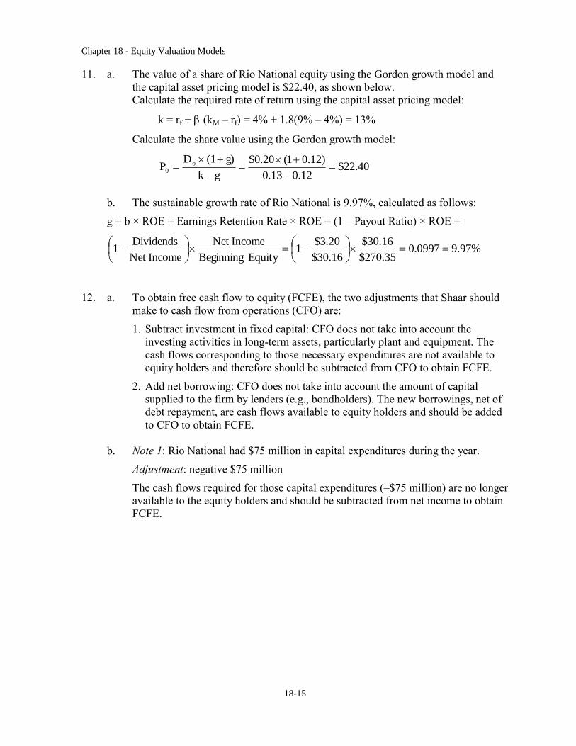
11. a. The value of a share of Rio National equity using the Gordon growth model and
the capital asset pricing model is $22.40, as shown below.
Calculate the required rate of return using the capital asset pricing model:
k = rf + (kM – rf) = 4% + 1.8(9% – 4%) = 13%
Calculate the share value using the Gordon growth model:
40.22$12.013.0
)12.01(20.0$
gk
g)(1DP o
0
b. The sustainable growth rate of Rio National is 9.97%, calculated as follows:
g = b × ROE = Earnings Retention Rate × ROE = (1 – Payout Ratio) × ROE =
%97.90997.035.270$
16.30$
16.30$
20.3$1
Equity Beginning
IncomeNet
IncomeNet
ividendsD1
12. a. To obtain free cash flow to equity (FCFE), the two adjustments that Shaar should
make to cash flow from operations (CFO) are:
1. Subtract investment in fixed capital: CFO does not take into account the
investing activities in long-term assets, particularly plant and equipment. The
cash flows corresponding to those necessary expenditures are not available to
equity holders and therefore should be subtracted from CFO to obtain FCFE.
2. Add net borrowing: CFO does not take into account the amount of capital
supplied to the firm by lenders (e.g., bondholders). The new borrowings, net of
debt repayment, are cash flows available to equity holders and should be added
to CFO to obtain FCFE.
b. Note 1: Rio National had $75 million in capital expenditures during the year.
Adjustment: negative $75 million
The cash flows required for those capital expenditures (–$75 million) are no longer
available to the equity holders and should be subtracted from net income to obtain
FCFE.
Chapter 18 - Equity Valuation Models
18-16
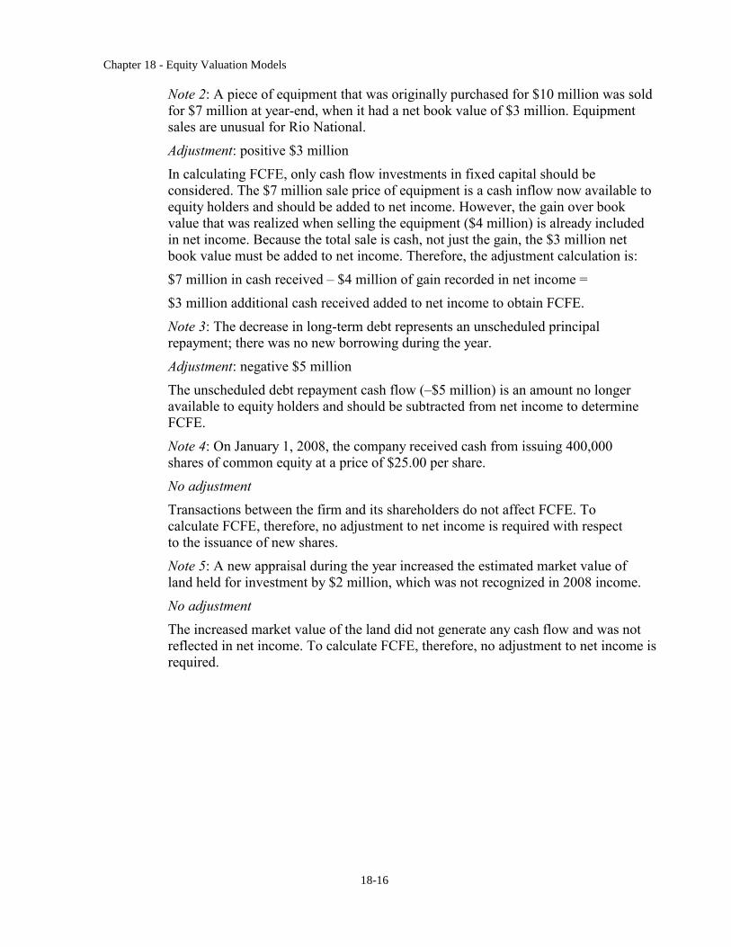
Note 2: A piece of equipment that was originally purchased for $10 million was sold
for $7 million at year-end, when it had a net book value of $3 million. Equipment
sales are unusual for Rio National.
Adjustment: positive $3 million
In calculating FCFE, only cash flow investments in fixed capital should be
considered. The $7 million sale price of equipment is a cash inflow now available to
equity holders and should be added to net income. However, the gain over book
value that was realized when selling the equipment ($4 million) is already included
in net income. Because the total sale is cash, not just the gain, the $3 million net
book value must be added to net income. Therefore, the adjustment calculation is:
$7 million in cash received – $4 million of gain recorded in net income =
$3 million additional cash received added to net income to obtain FCFE.
Note 3: The decrease in long-term debt represents an unscheduled principal
repayment; there was no new borrowing during the year.
Adjustment: negative $5 million
The unscheduled debt repayment cash flow (–$5 million) is an amount no longer
available to equity holders and should be subtracted from net income to determine
FCFE.
Note 4: On January 1, 2008, the company received cash from issuing 400,000
shares of common equity at a price of $25.00 per share.
No adjustment
Transactions between the firm and its shareholders do not affect FCFE. To
calculate FCFE, therefore, no adjustment to net income is required with respect
to the issuance of new shares.
Note 5: A new appraisal during the year increased the estimated market value of
land held for investment by $2 million, which was not recognized in 2008 income.
No adjustment
The increased market value of the land did not generate any cash flow and was not
reflected in net income. To calculate FCFE, therefore, no adjustment to net income is
required.
Chapter 18 - Equity Valuation Models
18-17
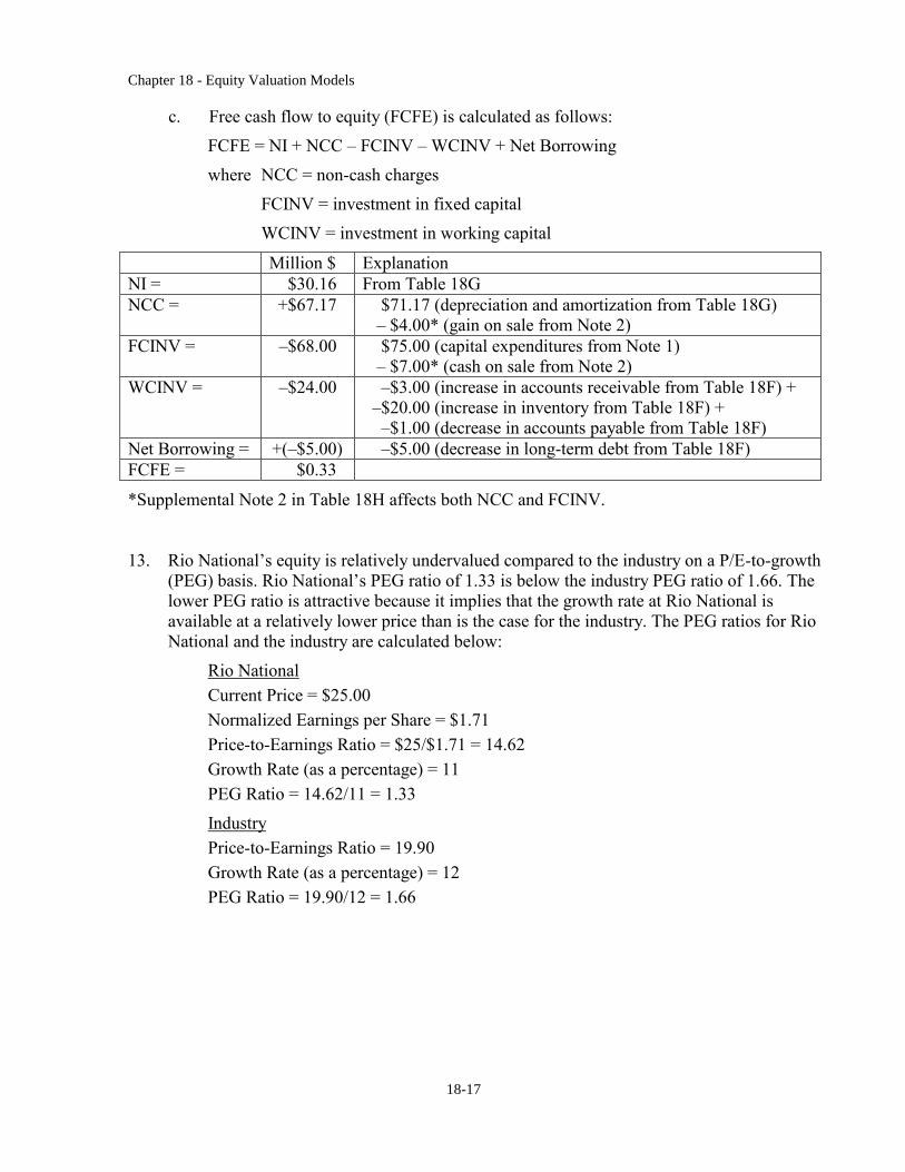
c. Free cash flow to equity (FCFE) is calculated as follows:
FCFE = NI + NCC – FCINV – WCINV + Net Borrowing
where NCC = non-cash charges
FCINV = investment in fixed capital
WCINV = investment in working capital
Million $ Explanation
NI = $30.16 From Table 18G
NCC = +$67.17 $71.17 (depreciation and amortization from Table 18G)
– $4.00* (gain on sale from Note 2)
FCINV = –$68.00 $75.00 (capital expenditures from Note 1)
– $7.00* (cash on sale from Note 2)
WCINV = –$24.00 –$3.00 (increase in accounts receivable from Table 18F) +
–$20.00 (increase in inventory from Table 18F) +
–$1.00 (decrease in accounts payable from Table 18F)
Net Borrowing = +(–$5.00) –$5.00 (decrease in long-term debt from Table 18F)
FCFE = $0.33
*Supplemental Note 2 in Table 18H affects both NCC and FCINV.
13. Rio National’s equity is relatively undervalued compared to the industry on a P/E-to-growth
(PEG) basis. Rio National’s PEG ratio of 1.33 is below the industry PEG ratio of 1.66. The
lower PEG ratio is attractive because it implies that the growth rate at Rio National is
available at a relatively lower price than is the case for the industry. The PEG ratios for Rio
National and the industry are calculated below:
Rio National
Current Price = $25.00
Normalized Earnings per Share = $1.71
Price-to-Earnings Ratio = $25/$1.71 = 14.62
Growth Rate (as a percentage) = 11
PEG Ratio = 14.62/11 = 1.33
Industry
Price-to-Earnings Ratio = 19.90
Growth Rate (as a percentage) = 12
PEG Ratio = 19.90/12 = 1.66