Chapter 17 Urban air pollution · Chapter 17 Urban air pollution ... Bart Ostro, Kiran Dev Pandey,...
82
Summary Current scientific evidence, derived largely from studies in North America and Western Europe (NAWE), indicates that urban air pollu- tion, 1 which is derived largely from combustion sources, causes a spec- trum of health effects ranging from eye irritation to death. Recent assessments suggest that the impacts on public health may be consider- able. This evidence has increasingly been used by national and interna- tional agencies to inform environmental policies, and quantification of the impact of air pollution on public health has gradually become a critical component in policy discussions as governments weigh options for the control of pollution. Quantifying the magnitude of these health impacts in cities world- wide, however, presents considerable challenges owing to the limited availability of information on both effects on health and on exposures to air pollution in many parts of the world. Man-made urban air pollu- tion is a complex mixture with many toxic components. We have chosen to index this mixture in terms of particulate matter (PM), a component that has been linked consistently with serious health effects, and, impor- tantly, levels of which can be estimated worldwide. Exposure to PM has been associated with a wide range of effects on health, but effects on mortality are arguably the most important, and are also most amenable to global assessment. Our estimates, therefore, consider only mortality. Currently, most epidemiological evidence and data on air quality that could be used for such estimates comes from developed countries. We have had, therefore, to make assumptions concerning factors such as the transferability of risk functions, exposure of the population and their underlying vulnerability to air pollution, while trying to ensure that these assumptions are transparent and that the uncertainty associated with them is assessed through appropriate sensitivity analyses. Chapter 17 Urban air pollution Aaron J. Cohen, H. Ross Anderson, Bart Ostro, Kiran Dev Pandey, Michal Krzyzanowski, Nino Künzli, Kersten Gutschmidt, C. Arden Pope III, Isabelle Romieu, Jonathan M. Samet and Kirk R. Smith
Transcript of Chapter 17 Urban air pollution · Chapter 17 Urban air pollution ... Bart Ostro, Kiran Dev Pandey,...

SummaryCurrent scientific evidence, derived largely from studies in NorthAmerica and Western Europe (NAWE), indicates that urban air pollu-tion,1 which is derived largely from combustion sources, causes a spec-trum of health effects ranging from eye irritation to death. Recentassessments suggest that the impacts on public health may be consider-able. This evidence has increasingly been used by national and interna-tional agencies to inform environmental policies, and quantification ofthe impact of air pollution on public health has gradually become a critical component in policy discussions as governments weigh optionsfor the control of pollution.
Quantifying the magnitude of these health impacts in cities world-wide, however, presents considerable challenges owing to the limitedavailability of information on both effects on health and on exposuresto air pollution in many parts of the world. Man-made urban air pollu-tion is a complex mixture with many toxic components. We have chosento index this mixture in terms of particulate matter (PM), a componentthat has been linked consistently with serious health effects, and, impor-tantly, levels of which can be estimated worldwide. Exposure to PM hasbeen associated with a wide range of effects on health, but effects onmortality are arguably the most important, and are also most amenableto global assessment. Our estimates, therefore, consider only mortality.Currently, most epidemiological evidence and data on air quality thatcould be used for such estimates comes from developed countries. Wehave had, therefore, to make assumptions concerning factors such as thetransferability of risk functions, exposure of the population and theirunderlying vulnerability to air pollution, while trying to ensure that theseassumptions are transparent and that the uncertainty associated withthem is assessed through appropriate sensitivity analyses.
Chapter 17
Urban air pollution
Aaron J. Cohen, H. Ross Anderson, Bart Ostro,Kiran Dev Pandey, Michal Krzyzanowski,Nino Künzli, Kersten Gutschmidt,C. Arden Pope III, Isabelle Romieu,Jonathan M. Samet and Kirk R. Smith

In order to provide estimates for all 14 subregions,2 models developedby the World Bank were used to estimate ambient concentrations ofinhalable particles (particulate matter with an aerodynamic diameter of<10mm, PM10) for PM in 3211 national capitals and cities with popula-tions of >100000 using economic, meteorological and demographic data and the available measurements. To allow the most appropriate epidemiological studies to be used for the estimation of the burden ofdisease, the estimates for PM10 were converted to estimates of fine particles (particulate matter with an aerodynamic diameter of <2.5mm,PM2.5) using available information on geographic variation in the ratioof PM2.5 to PM10. Population-weighted subregional annual average con-centrations of PM2.5 and PM10 were obtained using the population of thecities in the year 2000.
Our estimates of the burden of disease were based on the contribu-tions of three health outcomes: mortality from cardiopulmonary diseasein adults, mortality from lung cancer, and mortality from acute respira-tory infections (ARI) in children aged 0–4 years. Numbers of attribut-able deaths and years of life lost (YLL) for adults and children (aged 0–4years) were estimated using risk coefficients from a large cohort studyof adults in the United States of America (Pope et al. 2002) and a meta-analytical summary of five time-series studies of mortality in children,respectively. Base-case estimates were calculated assuming that the riskof death increases linearly over a range of annual average concentra-tions of PM2.5, between a counterfactual (or referent) concentration of7.5mg/m3 and a maximum of 50mg/m3.
The results indicate that the impact of urban air pollution on theburden of disease in the cities of the world is large, but this is likely tobe an underestimate of the actual burden, on the basis of an assessmentof sources of uncertainty. There is also considerable variation in ourestimates among the 14 subregions, with the greatest burden occurringin the more polluted and rapidly growing cities of developing countries.We estimated that air pollution in urban areas worldwide, in terms ofconcentrations of PM, causes about 3% of mortality attributable to car-diopulmonary disease in adults, about 5% of mortality attributable tocancers of the trachea, bronchus and lung, and about 1% of mortalityattributable to ARI in children. This amounts to about 0.80 million pre-mature deaths (1.4% of the global total) and 6.4 million YLL (0.7% ofthe global total). This burden occurs predominantly in developing coun-tries, with 39% of attributable YLL occurring in WPR-B and 20% inSEAR-D. The highest proportions of the total burden occurred in WPR-B and EUR-B, where urban air pollution caused 0.7–1.0% of the burdenof disease.
We quantified the statistical uncertainty of our base-case estimates byestimating the joint uncertainty in the estimates of annual average concentration of PM and the estimates of the relative risks. Estimatesworldwide and for most subregions vary by less than two-fold (50%
1354 Comparative Quantification of Health Risks
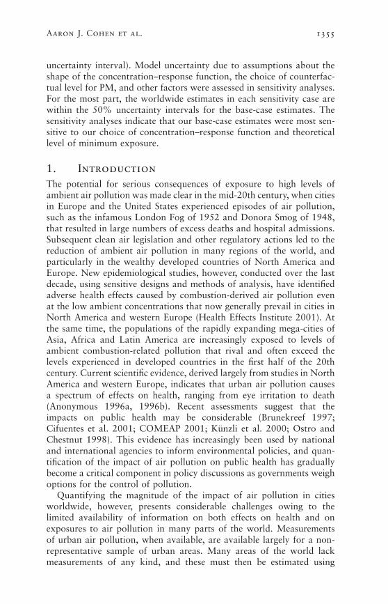
uncertainty interval). Model uncertainty due to assumptions about theshape of the concentration–response function, the choice of counterfac-tual level for PM, and other factors were assessed in sensitivity analyses.For the most part, the worldwide estimates in each sensitivity case arewithin the 50% uncertainty intervals for the base-case estimates. Thesensitivity analyses indicate that our base-case estimates were most sen-sitive to our choice of concentration–response function and theoreticallevel of minimum exposure.
1. IntroductionThe potential for serious consequences of exposure to high levels ofambient air pollution was made clear in the mid-20th century, when citiesin Europe and the United States experienced episodes of air pollution,such as the infamous London Fog of 1952 and Donora Smog of 1948,that resulted in large numbers of excess deaths and hospital admissions.Subsequent clean air legislation and other regulatory actions led to thereduction of ambient air pollution in many regions of the world, andparticularly in the wealthy developed countries of North America andEurope. New epidemiological studies, however, conducted over the lastdecade, using sensitive designs and methods of analysis, have identifiedadverse health effects caused by combustion-derived air pollution evenat the low ambient concentrations that now generally prevail in cities inNorth America and western Europe (Health Effects Institute 2001). Atthe same time, the populations of the rapidly expanding mega-cities ofAsia, Africa and Latin America are increasingly exposed to levels ofambient combustion-related pollution that rival and often exceed thelevels experienced in developed countries in the first half of the 20thcentury. Current scientific evidence, derived largely from studies in NorthAmerica and western Europe, indicates that urban air pollution causesa spectrum of effects on health, ranging from eye irritation to death(Anonymous 1996a, 1996b). Recent assessments suggest that theimpacts on public health may be considerable (Brunekreef 1997;Cifuentes et al. 2001; COMEAP 2001; Künzli et al. 2000; Ostro andChestnut 1998). This evidence has increasingly been used by nationaland international agencies to inform environmental policies, and quan-tification of the impact of air pollution on public health has graduallybecome a critical component in policy discussions as governments weighoptions for the control of pollution.
Quantifying the magnitude of the impact of air pollution in citiesworldwide, however, presents considerable challenges owing to thelimited availability of information on both effects on health and on exposures to air pollution in many parts of the world. Measurements of urban air pollution, when available, are available largely for a non-representative sample of urban areas. Many areas of the world lack measurements of any kind, and these must then be estimated using
Aaron J. Cohen et al. 1355
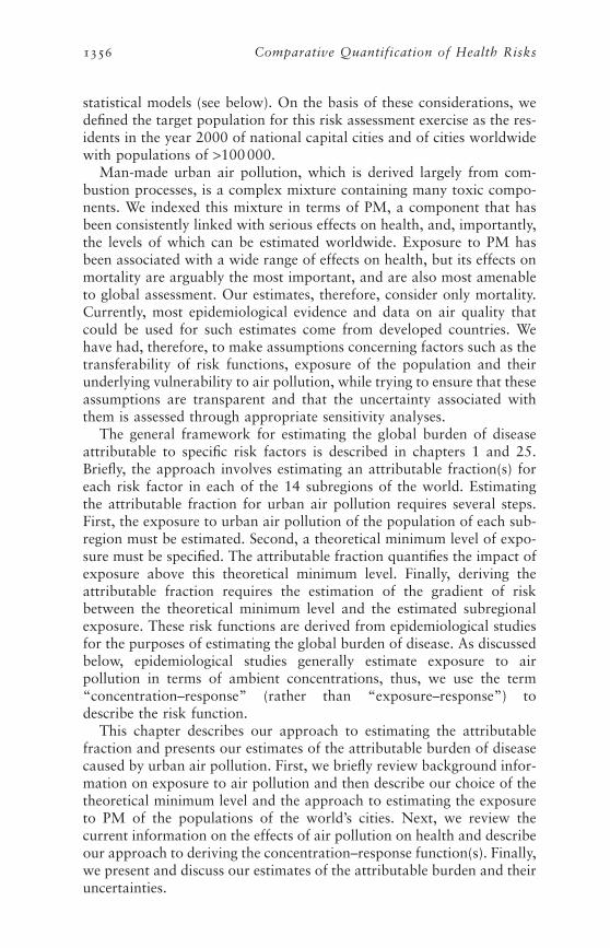
statistical models (see below). On the basis of these considerations, wedefined the target population for this risk assessment exercise as the res-idents in the year 2000 of national capital cities and of cities worldwidewith populations of >100000.
Man-made urban air pollution, which is derived largely from com-bustion processes, is a complex mixture containing many toxic compo-nents. We indexed this mixture in terms of PM, a component that hasbeen consistently linked with serious effects on health, and, importantly,the levels of which can be estimated worldwide. Exposure to PM hasbeen associated with a wide range of effects on health, but its effects onmortality are arguably the most important, and are also most amenableto global assessment. Our estimates, therefore, consider only mortality.Currently, most epidemiological evidence and data on air quality thatcould be used for such estimates come from developed countries. Wehave had, therefore, to make assumptions concerning factors such as thetransferability of risk functions, exposure of the population and theirunderlying vulnerability to air pollution, while trying to ensure that theseassumptions are transparent and that the uncertainty associated withthem is assessed through appropriate sensitivity analyses.
The general framework for estimating the global burden of diseaseattributable to specific risk factors is described in chapters 1 and 25.Briefly, the approach involves estimating an attributable fraction(s) foreach risk factor in each of the 14 subregions of the world. Estimatingthe attributable fraction for urban air pollution requires several steps.First, the exposure to urban air pollution of the population of each sub-region must be estimated. Second, a theoretical minimum level of expo-sure must be specified. The attributable fraction quantifies the impact ofexposure above this theoretical minimum level. Finally, deriving theattributable fraction requires the estimation of the gradient of riskbetween the theoretical minimum level and the estimated subregionalexposure. These risk functions are derived from epidemiological studiesfor the purposes of estimating the global burden of disease. As discussedbelow, epidemiological studies generally estimate exposure to air pollution in terms of ambient concentrations, thus, we use the term “concentration–response” (rather than “exposure–response”) todescribe the risk function.
This chapter describes our approach to estimating the attributablefraction and presents our estimates of the attributable burden of diseasecaused by urban air pollution. First, we briefly review background infor-mation on exposure to air pollution and then describe our choice of thetheoretical minimum level and the approach to estimating the exposureto PM of the populations of the world’s cities. Next, we review thecurrent information on the effects of air pollution on health and describeour approach to deriving the concentration–response function(s). Finally,we present and discuss our estimates of the attributable burden and theiruncertainties.
1356 Comparative Quantification of Health Risks

2. Exposure to urban air pollution fromcombustion sources
Combustion of fossil fuels for transportation, power generation, andother human activities produces a complex mixture of pollutants comprising literally thousands of chemical constituents (Derwent 1999;Holman 1999). Exposure to such mixtures is a ubiquitous feature ofurban life. The precise characteristics of the mixture in a given localedepend on the relative contributions of the different sources of pollution,such as vehicular traffic and power generation, and on the effects of thelocal geoclimatic factors. The relative contribution of different combus-tion sources is a function of economic, social and technological factors,but all mixtures contain certain primary gaseous pollutants, such assulfur dioxide (SO2), nitrogen oxides (NOX) and carbon monoxide (CO),that are emitted directly from combustion sources, as well as secondarypollutants, such as ozone (O3), that are formed in the atmosphere fromdirectly-emitted pollutants. The pollutant mixture also contains car-cinogens such as benzo(a)pyrene, benzene and 1,3-butadiene. Whenpetrol contains lead (Pb), as is still the case in many developing coun-tries, this element is a common constituent of the pollution mix, assessedin a separate chapter in this volume (chapter 19).
All combustion processes produce particles, most of which are smallenough to be inhaled into the lung either as primary emissions (such asdiesel soot), or as secondary particles via atmospheric transformation(such as sulfate particles formed from the burning of fuel containingsulfur). Their concentrations (in micrograms per cubic metre, or mg/m3)are generally measured as inhalable and fine particles, PM10 and PM2.5,respectively.3 However, the total suspended particle mass (TSP) is still the only particle measurement available in many developing countries(Krzyzanowski and Schwela 1999).
Pollution from the combustion of fossil fuels is largely emitted intothe outdoor air, but human exposure occurs both indoors and outdoors(Ozkaynak 1999). An individual’s exposure to ambient urban air pollu-tion depends on the relative amounts of time spent indoors and outdoors,the proximity to sources of ambient air pollution, and on the indoor con-centration of outdoor pollutants. The indoor concentrations depend onfactors such as the circulation of the indoor air and the degree to whichconstituents of the outdoor combustion mixture penetrate and persist inthe indoor environment. Studies conducted largely in Europe and NorthAmerica have shown that the fine particles generated from combustionoutdoors both effectively penetrate and persist in many indoor environ-ments. Gases, such as sulfur dioxide and ozone, may penetrate the indoorenvironment, but generally do not persist because of their reactivity. Insome rural areas of developing countries, indoor cooking on unventedcoal- or biomass-burning stoves is the most significant exposure to pollution from combustion sources. The burden of disease caused by
Aaron J. Cohen et al. 1357

such exposure is addressed in chapter 18. The actual dose delivered tothe lung or other organs will further depend on the type of pollutant,the breathing pattern and physical characteristics of the individual thatdetermine the extent and site of deposition.
Governments in many parts of the world monitor ambient concen-trations of air pollution as part of regulatory programmes designed toprotect public health and the environment (Grant et al. 1999). The mostextensive monitoring systems are in the United States and westernEurope, where regular monitoring of ambient air quality has been inplace since the mid-1970s. The most frequently and routinely monitoredair pollutants include sulfur dioxide (SO2), nitrogen oxides (NOX, includ-ing NO and NO2), carbon monoxide (CO), ozone (O3), lead (Pb), blacksmoke (BS) or soot, and PM. National monitoring systems also exist inother parts of the world, but access to the data collected by these systemsand international standardization of the monitoring methods are limited.The World Health Organization (WHO) Air Management InformationSystem (AMIS) (WHO 2001c) collects the available information, but thereporting from many regions is poor, and for some regions there are nodata in the WHO database. The various designs of the networks, dif-ferences in monitoring objectives and limited availability of the collecteddata for the outside users limit access to the information on populationexposure in the greater proportion of the world’s cities. In some parts ofthe world (e.g. in most of the countries of the former Soviet Union), themonitoring systems exist but do not provide the data necessary forassessment of the impact on health (Krzyzanowski and Schwela 1999).More details about the data available for this analysis are provided infurther sections of this chapter.
These monitoring systems currently provide much of the data onexposure to urban air pollution that have been used in epidemiologicalresearch, although some studies establish their own monitoring networkswhen routinely-collected data are either unavailable or of poor quality,or to measure specific air pollution constituents, such as specific knowncarcinogens. Typically, monitoring sites are located in the city centre orthroughout a given metropolitan area, in order to more accurately reflectthe average residential exposure of the population. The data from mon-itors sited so as to measure emissions from specific sources, such as alocal industry or heavy vehicular traffic, are frequently excluded fromthe data sets, as they may significantly deviate from the average levels ofexposure experienced by the population.
Exposure estimates that rely exclusively on data from one or morestationary monitoring sites may provide inaccurate estimates of theshort- and/or long-term average personal exposures of study populations(Navidi and Lurmann 1995; Zeger et al. 2000). The direction and mag-nitude of the errors that will be induced in estimates of the relative riskattributable to exposure to air pollution depend on the precision of theair quality monitoring data (or models used to generate the estimates of
1358 Comparative Quantification of Health Risks

the concentration of pollution), the applicability of one estimate to theentire target population and the correlation of the errors with the healthoutcome. Generally, such errors will be smaller for pollutants that tendto be uniformly distributed over large urban areas, and that penetrateefficiently indoors, both of these features being the case for fine PM produced by combustion. If the errors in the estimates of exposure areuncorrelated with the risk of the health outcome, then the estimates ofrelative risk attributable to air pollution will, in most cases, be too low(i.e. biased to the null) (Navidi and Lurmann 1995).
2.1 Definition of the air pollution metric for exposure variable
We selected PM10 and PM2.5 as the indicators of exposure to urban air pollution from combustion sources. As noted above, PM is a ubiquitouscomponent of the mixtures emitted into, and formed in, the ambient envi-ronment by combustion processes, and indicates the presence of these mix-tures in outdoor air. Most importantly, these measures of particulate airpollution have been used in many epidemiological studies from aroundthe world, of both mortality and morbidity of air pollution, and so providethe best overall indicator of exposure for our purposes (see section 3).Although other components of ambient air pollution from combustionsources are associated with these and other effects on health (Anonymous1996a, 1996b), particulate air pollution has been found to be consistentlyand independently related to the most serious effects of air pollution,including daily and longer-term average mortality (California AirResources Board 2002; Health Effects Institute 2001; U.S. EnvironmentalProtection Agency 2002; WHO 2000a, 2003). There is some evidence,although much less than that for PM, linking ozone to premature mor-tality, particularly during the summer months (Abbey et al. 1999; HealthEffects Institute 2000b). However, despite recent progress in developingmodels to estimate tropospheric (ground-level) ozone on a global scale, itwas not currently feasible to derive the subregional estimates that wouldhave been required for this project. In many developing countries, expo-sure to lead in the ambient air may also be of great consequence, havingeffects on mortality perhaps via effects on blood pressure. The impacts oflead in outdoor air are dealt with in chapter 19.
PM has been linked to serious effects on health after both short-termexposure (days to weeks), and more prolonged exposure (years),although there remains some uncertainty as to the distribution of induc-tion times with regard to mortality (see below). We chose the annualaverage concentration(s) of PM as the exposure metric(s) because it cor-responds to the time-scales of a priori interest for estimates of attribut-able and avoidable burden in the Global Burden of Disease (GBD)project, and because it was used to estimate the effects of exposure toPM in the key epidemiological study that provides our estimates of theconcentration–response function.
Aaron J. Cohen et al. 1359
2.2 Estimation of annual average concentrations ofparticulate matter
AIR POLLUTION MEASUREMENTS USED IN ESTIMATING ANNUAL
AVERAGE CONCENTRATIONS
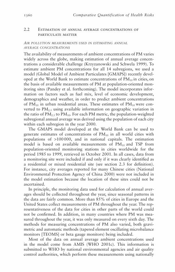
The availability of measurements of ambient concentrations of PM varieswidely across the globe, making estimation of annual average concen-trations a considerable challenge (Krzyzanowski and Schwela 1999). Toestimate ambient PM concentrations for all 14 subregions, we used amodel (Global Model of Ambient Particulates [GMAPS]) recently devel-oped at the World Bank to estimate concentrations of PM10 in cities, onthe basis of available measurements of PM at population-oriented mon-itoring sites (Pandey et al. forthcoming). The model incorporates infor-mation on factors such as fuel mix, level of economic development,demographics and weather, in order to predict ambient concentrationsof PM10 in urban residential areas. These estimates of PM10 were con-verted to PM2.5 using available information on geographic variation inthe ratio of PM2.5 to PM10. For each PM metric, the population-weightedsubregional annual average was derived using the population of each citywithin each subregion in the year 2000.
The GMAPS model developed at the World Bank can be used to generate estimates of concentrations of PM10 in all world cities with populations of >100000, and in national capitals. The estimation model is based on available measurements of PM10 and TSP from population-oriented monitoring stations in cities worldwide for theperiod 1985 to 1999, retrieved in October 2001. In all cases, data froma monitoring site were included if and only if it was clearly identified asa residential or mixed residential site (see section 2.3 for definition). For instance, city averages reported for many Chinese cities (NationalEnvironmental Protection Agency of China 2000) were not included inthe model estimation because the location of these sites could not beascertained.
In principle, the monitoring data used for calculation of annual aver-ages should be collected throughout the year, since seasonal patterns inthe data are fairly common. More than 85% of cities in Europe and theUnited States collect measurements of PM throughout the year. The rep-resentativeness of the data for cities in other parts of the world couldnot be confirmed. In addition, in many countries where PM was mea-sured throughout the year, it was only measured on every sixth day. Themethods for measuring concentrations of PM also varied, both gravi-metric and automatic methods (tapered element oscillating microbalancemonitors [TEOMS] or beta gauge monitors) being included.
Most of the data on annual average ambient concentrations used in the model come from AMIS (WHO 2001c). This information is submitted to WHO by national environmental agencies and air qualitycontrol authorities, which perform these measurements using nationally
1360 Comparative Quantification of Health Risks

approved methods and standards of data quality. The data set containsthe annual mean concentration of selected air pollutants, including PM,by monitoring site. Additional data, such as 95th percentiles of dailymeans, are also available for some sites. Although WHO requests thatall Member States provide data for compilation in the AMIS database,the reported data are still limited because many countries do not haveair quality monitoring networks. Additionally, some countries with mon-itoring networks may not report the data because of poor data qualityor limited ability to process and report the data.
The data from AMIS were supplemented with other sources of data on TSP and PM10 from monitoring sites. These included data forEuropean cities collected by WHO/European Centre for Environ-ment and Health (ECEH) for the Health Impact Assessment of Air Pollution (HIAAP) project in 1999 from both national and local environmental agencies (WHO 2001a), data for Canadian cities pro-vided by Environment Canada (www.ec.gc.ca) and statistics Canada(http://www.statcan.ca/english/ads/cansimII/index.htm), and data forcities in the United States from the U.S. Environmental Protection AgencyAIRS database (Aerometric Information Retrieval System 2001). Datafor Chinese cities were also obtained from the Environmental QualityReports from China (National Environmental Protection Agency ofChina 2000), and Mexican cities from the Instituto Nacional de Ecología(INE), SEMARNAP, Mexico (Instituto Nacional de Ecología 2000).Additional data were also obtained from the World Bank URBAIRstudies of air pollution in Jakarta and Kathmandu (Grønskei et al.1997a, 1997b). To limit undue influence of the data from cities in theUnited States, data used from the United States AIRS database werelimited to the years 1996–1999.4
Measured annual average concentrations of PM10 and TSP data frommonitoring sites were available for 512 unique locations in 304 cities in 55 countries over the period 1985–1999, and provided 1997 time–location data points. For some sites and years, data on both TSP andPM10 were available, yielding a total of 2344 individual observations.5
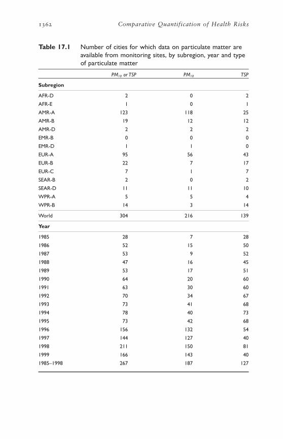
The number of cities with measured data on PM from monitoring sitesin each subregion and for each year by PM measure is shown in Table17.1. A total of 304 cities reported either the annual average concen-trations of PM10 or TSP for at least 1 year between 1985 and 1999. Ofthese, 51 cities reported both PM10 and TSP while 165 cities, mostly inNorth America and western Europe, reported PM10 only, and the remain-ing 88 cities reported data for TSP only.
Coverage of cities and populations with data from monitoring sitesvaries significantly across different subregions (Figure 17.1). Forinstance, data from monitoring were available for fewer than two citiesfor six of the subregions, AFR-D, AFR-E, AMR-D, EMR-B, EMR-D andSEAR-B. In contrast, data from monitoring sites were available for 218cities in NAWE, of which 174 report data on PM10. The 304 world cities
Aaron J. Cohen et al. 1361
1362 Comparative Quantification of Health Risks
Table 17.1 Number of cities for which data on particulate matter areavailable from monitoring sites, by subregion, year and typeof particulate matter
PM10 or TSP PM10 TSP
Subregion
AFR-D 2 0 2
AFR-E 1 0 1
AMR-A 123 118 25
AMR-B 19 12 12
AMR-D 2 2 2
EMR-B 0 0 0
EMR-D 1 1 0
EUR-A 95 56 43
EUR-B 22 7 17
EUR-C 7 1 7
SEAR-B 2 0 2
SEAR-D 11 11 10
WPR-A 5 5 4
WPR-B 14 3 14
World 304 216 139
Year
1985 28 7 28
1986 52 15 50
1987 53 9 52
1988 47 16 45
1989 53 17 51
1990 64 20 60
1991 63 30 60
1992 70 34 67
1993 73 41 68
1994 78 40 73
1995 73 42 68
1996 156 132 54
1997 144 127 40
1998 211 150 81
1999 166 143 40
1985–1998 267 187 127
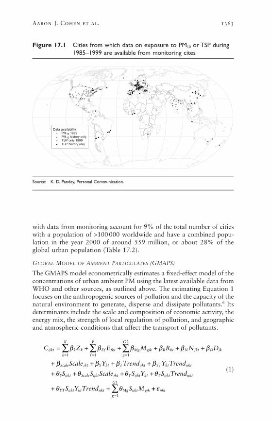
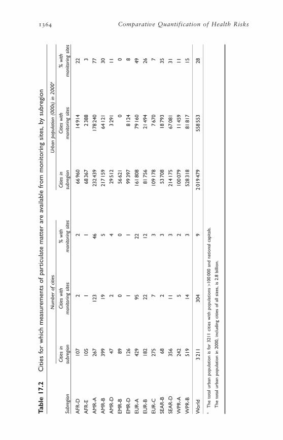
with data from monitoring account for 9% of the total number of citieswith a population of >100000 worldwide and have a combined popu-lation in the year 2000 of around 559 million, or about 28% of theglobal urban population (Table 17.2).
GLOBAL MODEL OF AMBIENT PARTICULATES (GMAPS)
The GMAPS model econometrically estimates a fixed-effect model of theconcentrations of urban ambient PM using the latest available data fromWHO and other sources, as outlined above. The estimating Equation 1focuses on the anthropogenic sources of pollution and the capacity of thenatural environment to generate, disperse and dissipate pollutants.6 Itsdeterminants include the scale and composition of economic activity, theenergy mix, the strength of local regulation of pollution, and geographicand atmospheric conditions that affect the transport of pollutants.
(1)
C Z E M R N D
Scale Y Trend Y Trend
S S Scale S Y S Trend
S Y Trend S M
ijkt k kk
K
Ef fktf
F
Mg gikg
G
R kt N jkt D jk
Scale jkt Y kt T ijkt YT kt ijkt
S ijkt Scale ijkt jkt Y ijkt kt T ijkt ijkt
YT ijkt kt ijkt Mg ijkt gjk
= + + + + +
+ + + ++ + + +
+ +
= = =Â Â Âb b b b b b
b b b bq q q q
q q
1 1 1
2
++=
 e ijktg
G
1
1
Aaron J. Cohen et al. 1363
Figure 17.1 Cities from which data on exposure to PM10 or TSP during1985–1999 are available from monitoring cites
PM10 1999
TSP only 1999TSP history only
PM10 history only
Source: K. D. Pandey, Personal Communication.
1364 Comparative Quantification of Health Risks
Tabl
e 17
.2C
ities
for
whi
ch m
easu
rem
ents
of
part
icul
ate
mat
ter
are
avai
labl
e fr
om m
onito
ring
site
s,by
sub
regi
on
Num
ber
of c
ities
Urb
an p
opul
atio
n (0
00s)
in 2
000a
Citie
s in
Ci
ties
with
%
with
Ci
ties
in
Citie
s w
ith
% w
ith
Subr
egio
nsu
breg
ion
mon
itorin
g sit
esm
onito
ring
sites
subr
egio
nm
onito
ring
sites
mon
itorin
g sit
es
AFR
-D10
72
266
960
1491
422
AFR
-E10
51
168
367
238
83
AM
R-A
267
123
4623
243
917
824
077
AM
R-B
399
195
217
159
6412
130
AM
R-D
472
429
512
329
111
EMR
-B89
00
5662
10
0
EMR
-D12
61
199
397
812
48
EUR
-A42
995
2216
180
879
160
49
EUR
-B18
222
1281
756
2149
426
EUR
-C27
57
310
917
87
670
7
SEA
R-B
682
353
708
1879
335
SEA
R-D
356
113
214
175
6708
131
WPR
-A24
25
210
007
911
459
11
WPR
-B51
914
352
831
881
817
15
Wor
ld3
211
304
92
019
479
558
553
28
aT
he t
otal
urb
an p
opul
atio
n is
for
3211
citi
es w
ith p
opul
atio
ns >
100
000
and
natio
nal c
apita
ls.
The
tot
al u
rban
pop
ulat
ion
in 2
000,
incl
udin
g ci
ties
of a
ll si
zes,
is 2
.8 b
illio
n.

where
Cijkt = log of concentration of PM in monitoring station i, city j,country k, at time t
Zk = binary variable for country k
Efkt = log of per capita energy consumption of energy source type ffor country k at time t (f=1 . . . F)
Mgjk = log of meteorological/geographic factor g for city j, country k(factors g=1 . . . G1 affect PM10 concentration in a differentway than TSP concentration. Factors g=G1+1 . . . G2 do notmake a distinction between PM10 and TSP)
Rkt = log of population density of country k at time t
Njkt = log of population of city j, country k, at time t
Djk = log of local population density in the vicinity of city j incountry k
Scalejkt = log of scale of economy (intensity of economic activity) forcity j, country k at time t
Ykt = log of income per capita (1-year lagged 3-year movingaverage) of country k at time t
Trendijkt = time trend (1985=1, 1986=2, . . . 1999=15)
Sijkt = binary variable for PM type measured at monitoring stationi, city j, country k, at time t, (1=TSP, 0=PM10), and
the bS and qS are the parameters that are estimated by the model.Equation 1 jointly determines the concentrations of total suspended
particulate matter (TSP) and inhalable particulates (PM10) in residentialareas. Most cities in developing countries only monitor TSP and notPM10. Adoption of the pooled specification permits use of all availabledata and provides better information about the concentrations of PM,especially for cities in developing countries. Limiting the estimationsample to PM10 observations is sensible only if knowledge of the con-centration of TSP in a city makes no contribution to predicting PM10.Since PM10 comprises the smaller size particles within TSP, this assump-tion is clearly unreasonable. The pooled specification allows for separateestimation of concentrations of PM10 and TSP for each city by settingthe binary variable, Sijkt, equal to zero or one, as shown in Equations 2and 3.
(2)log PM Z E M R N
D Scale Y Trend Y Trend
ijkt k kk
K
Ef fktf
F
Mg gjkg
G
R kt N jkt
D jk Scale jkt Y kt T ijkt YT kt ijkt
101 1 1
2
[ ] = + + + +
+ + + + += = =
  Âb b b b b
b b b b b
Aaron J. Cohen et al. 1365

(3)
To reduce undue influence from extreme values, all of the continuousvariables in the model were specified in log form and each exogenousvariable in the estimation sample was truncated to the middle 98% rangeobserved in the estimation sample.
The estimation Equation 1 includes country-specific binary variables,Zk, to control for economic, social and natural factors that are not cap-tured by the other explanatory variables. These include differences in the quality of the data on ambient concentration and in collectionmethods across countries, the degree of regulatory heterogeneity withina country, the relative importance of intercity transport, proximity of and pollution levels in neighbouring cities and the composition of economic activity. The country-specific binary variables measure theaverage concentration of PM in each country during the 15-year period1986–1999, controlling for variations within the country caused byfactors accounted for in the remainder of the estimating Equation 1. Incontrast, the rest of the estimation model (1) explains the marginal con-tribution of the included factors to deviations in the ambient concentra-tion in the city from this average.
The primary determinants of the observed variations in the ambientconcentrations of PM within a country in the estimation model are:
Energy consumption. The model includes six separate per capitaenergy consumption categories—coal, oil, natural gas, nuclear, hydro-electric, combustible renewables and wastes—that account for all energyconsumed in each country for which data are available from the International Energy Agency’s (IEA) Annual Energy Balance database(International Energy Agency 2001a, 2001b). The separate inclusion ofeach type of energy source accounts for differences in emission factors,variations in economic activity and intensity of fuel use across countries.In addition, the model also includes per capita consumption of petroland diesel used in the transportation sector, also available from IEA’sdatabase, to capture additional detail about one of the most significantcontributors to ambient concentrations of PM.
Meteorological and geographic factors. The model includes 22 atmos-pheric and geographic factors for each city to account for both the dissipative/dispersive capacity of the natural environment and naturalsources of particulates, such as desert dust storms, forest fires and seaspray. These include a suite of 18 climatic variables representing the long-
log TSP Z E M R N
D Scale Y Trend Y Trend
Scale Y Trend Y Trend
M
ijkt k kk
K
Ef fktf
F
Mg gjkg
G
R kt N jkt
D jk Scale jkt Y kt T ijkt YT kt ijkt
S Scale jkt Y kt T ijkt YT kt ijkt
Mg gjkg
G
[ ] = + + + +
+ + + + ++ + + + +
+
= = =
=
  Â
Â
b b b b b
b b b b bq q q q q
q
1 1 1
2
1
1
1366 Comparative Quantification of Health Risks

term average climatic conditions related to local atmospheric conditionsand transport of PM, consisting of the annual average (average of themonthly data) and seasonal changes (measured as the standard devia-tion of the monthly data) for the following nine factors: mean tempera-ture, diurnal temperature, mean precipitation, barometric pressure, windspeed, percentage cloud cover and frequency of wet, sunny and frostydays (New et al. 1999).7 In addition, two meteorological variables relatedto energy demand (heating and cooling degree-days) are estimated foreach city from the mean monthly temperature. Two topographical vari-ables related to atmospheric transport—distance from the city centre tothe nearest point on the coastline, calculated using the geographic infor-mation system (GIS), and elevation of the city, derived from a globaldigital elevation model (USGS 1996)—are also included in the model.
City and national population and national population density. Thesevariables provide measures of the scale and intensity of the pollutionproblem in each city. The data on population comes from the Demo-graphic yearbook published by the United Nations (UN 2001).
Local population density. The local population density in the vicinityof each city provides a measure of the intensity of pollution. It is esti-mated from the Gridded Population of the World (version 2), availablefrom the Consortium for International Earth Science InformationNetwork (CIESIN 2000). This data set provides the best available population data for about 120000 administrative units, converted to aregular grid of population counts at a resolution of about 5km. The localpopulation density in the vicinity of each city is the average populationdensity for all grid cells within a 20-km radius of the city centre.
Local intensity of economic activity. Most cities do not collect dataon the amount or composition of economic activity. Instead, the localgross domestic product (GDP) per square kilometre computed as theproduct of the national per capita GDP and the local population densityin the vicinity of each city is used as a proxy for the intensity of eco-nomic activity within each city (World Bank 2002).
National income per capita. This variable is used to capture the following national indicators: valuation of the quality of the environ-ment, strength of environmental policy and regulation, the institutionalcapacity to enforce environmental policies, and the potential use ofcleaner fuels along the fuel-use chain as countries develop. It is measuredas a 1-year lag of the average of the previous 3 years (World Bank 2002).
Time trends. The model includes two time-trend variables (with 1985=1 . . . 1999=15) to allow for differential time trends for PM10 andTSP particulate pollution. Both of these variables are in turn interactedwith lagged national per capita income to allow trends to vary acrosscountries on the basis of differential valuation and improvements in envi-ronmental quality across countries as measured by the level of economicdevelopment. These trends measure changes in concentrations of PM
Aaron J. Cohen et al. 1367
that are caused by factors not already captured in the model, such astechnological changes, improvements in knowledge and structural shiftsin the composition of economic activity. They do not represent theunconditional aggregate trends in concentrations of PM.
Binary variable to differentiate PM10 and TSP. The model includes abinary variable indicating whether PM is measured as TSP or PM10. Thisbinary variable is also allowed to interact in the model with other vari-ables to allow for size class differences in the composition of particulatesacross cities and countries. It provides a better representation of inter-city differences across the world, rather than assuming a uniform rela-tionship across all cities. The log of the ratio of PM10 to TSP in each citycan be estimated by subtracting Equation 3 from 2, as shown in Equa-tion 4. The key determinants of this ratio are the scale of economic activ-ity, differential trends across countries, level of economic developmentand strength of environmental policy, and the subset of meteorologicalvariables that are directly related to particle size (annual mean and seasonal variations in wind speed, precipitation and frequency of wetdays).
(4)
In order to facilitate predictions for countries not included in the esti-mation, a secondary model shown in Equation 5 is estimated to explainthe average level of ambient PM concentration in each country.
(5)
where
= country-specific binary variable coefficient estimated in Equation 1
= log of average per capita energy consumption of energy type f forcountry k during 1985–1999 (f = 1 . . . F)
= log of average population density of country k during 1985–1999
= log of average national per capita income of country k during1985–1999 (1-year lagged average of previous 3 years)
This secondary model (5) explains the average level of pollution underreference conditions for a country, on the basis of the scale of theeconomy, the composition of economic activity as measured by theenergy mix, and the strength of local pollution regulations and the insti-tutional capacity for implementing these regulations.
Yk
Rk
Efk
)bk
)b g g gk Ef fk R k R k k
f
F
E R Y u= + + +=
Â1
log logPM TSP Scale Y
Trend Y Trend M
ijkt ijkt S Scale jkt Y kt
T ijkt YT kt ijkt Mg gjkg
G
10
1
1
[ ] - [ ] = - - -
- - -=
Â
q q q
q q q
1368 Comparative Quantification of Health Risks

2.3 Model outputs
The GMAPS model is designed to obtain the best city-level prediction ofconcentrations of PM for a wide range of cities on the basis of the limitedamount of data from monitoring available, so it focuses on increasingthe fit of the model. It is not designed to provide a causal model forambient concentrations of air pollution. The estimation model (1)explains 88% of the variation in the observed data from monitoring,indicating a good fit (Pandey et al. forthcoming). The overall correlationbetween the measured and the predicted data is around 0.9 for both PM10
and TSP observations (see Table 17.3), and is >0.80 for all years and forboth observations of PM10 and TSP, with the exception of PM10 in 1985.The correlation by subregion is smaller than that over time, rangingbetween 0.2 and 0.9 for subregions with more than 10 data points. Thecorrelations for subregions with fewer data points are smaller than 0.2and are less precisely estimated. A negative correlation for EUR-B isdriven by a single erroneous observation for Bucharest, Romania, wherethe observed concentration of PM10 is higher than that of TSP. Theseresults originated from two different monitoring locations; had themodel been re-estimated without this particular PM10 observation, thecorrelation for the subregion would have been 0.32.
Subregion- and PM type-specific scatter plots of model predictionscompared to actual data also show a clustering of points around the solidline drawn at a 45∞ angle, indicating that the actual values are close tothe predicted values. As would be expected, the predicted values are lessextreme than the actual values at both tails, owing to the truncation ofall explanatory variables to the middle 98% range of the estimationsample. F-tests revealed that all of the eight aggregate factors in themodel added significant explanatory power to the regression.
The secondary estimation model (5) explains 85% of the variation inthe estimated average level of pollution in a country, indicating that thismodel provides a good fit. The explanatory power of the secondarymodel is not as robust to changes in the estimation sample owing to significant uncertainties in the estimated dependent variable.
Out-of-sample predictions were used to validate the model using bothstatistical and heuristic criteria. The model was re-estimated using sub-samples of the data on the basis of different cut-off points for per capitaincome, to examine the appropriateness of extrapolating from a modelprimarily based on industrialized cities in North America and westernEurope to cities in developing countries. The resulting estimates from themodel were used to predict concentrations of PM10 in residential areasin the out-of-sample cities located in developing countries. A second setof estimates was also made comprising income-based subsamples usingonly the available data on PM10 from monitoring in residential sites.These validation estimates consistently showed that out-of-sample cor-relations were higher when data on TSP were included in the estima-tions. Furthermore, the out-of-sample correlations on aggregate ranged
Aaron J. Cohen et al. 1369

1370 Comparative Quantification of Health Risks
Table 17.3 Correlation between observed concentrations of particulatematter at monitoring sites and predictions by subregion,year and type of particulate matter
PM10 or TSP PM10 TSP
No. of No. of No. of observations Correlation observations Correlation observations Correlation
Subregion
AFR-D 6 0.86 0 NA 6 0.86
AFR-E 2 –1.00 0 NA 2 –1.00
AMR-A 1 273 0.79 938 0.59 335 0.67
AMR-B 361 0.80 215 0.52 146 0.75
AMR-D 34 0.88 18 0.31 16 0.72
EMR-D 1 NA 1 NA 0 NA
EUR-A 182 0.85 75 0.82 107 0.73
EUR-B 63 0.83 16 –0.29 47 0.78
EUR-C 54 0.84 1 NA 53 0.83
SEAR-B 9 0.14 0 NA 9 0.14
SEAR-D 158 0.81 65 0.69 93 0.80
WPR-A 69 0.85 36 0.86 33 0.20
WPR-B 132 0.92 21 0.49 111 0.89
World 2 344 0.94 1 386 0.89 958 0.92
Year
1985 35 0.95 7 0.11 28 0.85
1986 68 0.93 17 0.81 51 0.92
1987 65 0.93 11 0.94 54 0.92
1988 70 0.93 20 0.91 50 0.92
1989 76 0.94 21 0.90 55 0.94
1990 91 0.94 24 0.90 67 0.94
1991 101 0.96 34 0.94 67 0.95
1992 116 0.94 38 0.95 78 0.93
1993 130 0.94 49 0.95 81 0.92
1994 138 0.94 46 0.94 92 0.93
1995 144 0.94 59 0.94 85 0.93
1996 330 0.92 259 0.88 71 0.90
1997 298 0.89 253 0.79 45 0.92
1998 377 0.88 289 0.84 88 0.84
1999 305 0.90 259 0.83 46 0.87
All years 2 039 0.94 1 127 0.90 912 0.92except 1999
NA Not applicable.

between 0.40 and 0.59, based on the income cut-off used, and lendsupport to the modelling approach.
Since cities with data from monitoring are not representative of allcities and account for a small fraction of urban residents in developingcountries, the following heuristic criteria were also used to evaluate thepredictions of the model.
• Comparison of the relative variation of the predictions within coun-tries and between countries relative to the actual data: The model predictions exhibited significant variations both across countries and across cities within a country. The predicted variations within acountry were about 60% of those between countries and were com-parable to the corresponding variations in the actual data.
• Number of cities for which predictions were outside the range of theestimation sample: The predictions for PM10 were within the rangeobserved in the actual data. They continued to be within bounds whenthe same fractions of values are removed from the tails of the esti-mated and measured data.
• Magnitude of predictions outside the range observed in the estimationsample: Of the 304 cities with data from monitoring, concentrationsof PM10 exceeded 200mg/m3 in three cities and concentrations of TSPexceeded 400mg/m3 in 10 cities. The predicted concentrations of PM10
exceeded 200mg/m3 in only four out of 3226 cities.
• Range of the PM10 :TSP ratio: The PM10 :TSP ratio predicted by the model is between 0.24 and 0.98 and spans the middle 95% of therange observed in the actual data. The mean ratio predicted by themodel is 0.49; the ratio for half of the cities lies between 0.39 and0.56.
• Comparison of the uncertainty in estimates for cities, relative to theamount of available information for neighbouring cities: Bootstraperror estimates of the prediction error for the city showed that theconfidence intervals were wider for cities with no data from monitoring and are largest in the countries with no data from monitoring.
The robustness of the model was tested using alternative specificationsof the model based on the goodness-of-fit of the model and the heuris-tic criteria outlined above. The alternative models that were consideredwere:
• Linear model. The linear model provides undue weight to the extremevalues in the explanatory variables, resulting in predictions that areorders of magnitude larger than those for cities with data from monitoring.
Aaron J. Cohen et al. 1371

• Explanatory variable truncation. The model was re-estimated withfour different levels of truncation for the explanatory variables: notruncation, truncation to the actual range for the cities with data frommonitoring, truncation to the middle 98% range of all explanatoryvariables for these cities, and truncation to the middle 90% range forthese cities. Estimates based on the first two of these were sensitive tosome of the extreme data points in the estimation sample, resultingin large variations in the predictions. Estimates from the last trunca-tion were rejected because more than one quarter of the observationswere truncated, leading to a poorer model fit.
• Energy consumption variables. The model was re-estimated with threealternative measures for the energy consumption variables: energyconsumption per area, total per capita energy consumption and shareof each energy type in the total energy mix, and the product ofnational per capita energy consumption by energy type and city pop-ulation density. The specification per area resulted in predictions thatwere unstable and orders of magnitude larger than those observed inany city because of truncation of extreme values in countries withmissing data on fuels. The second and third specifications resulted inpoorer fits with over-predictions for >100 cities with values outsideof the observed range of concentrations of PM10.
• Income. The model was estimated using income-squared and income-cubed terms to measure the impact of national per capita income.Higher order terms were unstable and resulted in predictions thatwere orders of magnitude larger than those observed in any city.
• PM10 :TSP ratio. A number of different models were estimated from full interactivity of the binary variable Sijkt with all of the continuous variables, to no interactivity with the continuous vari-ables. The full interactivity model was rejected because it predictedphysically implausible PM10 :TSP ratios of 2 for a significant number of cities. The limited model with no interactivity was rejectedbecause it over-predicted the results for many cities in the Middle Eastand North Africa that contain a larger fraction of wind-blown coarserparticles. Other models were estimated that incrementally addedgroups of variables, such as energy type and the other climate vari-ables. These were all rejected using the heuristic criteria outlinedabove.
• Location of monitoring sites. The sensitivity of the model predictionsto the inclusion of mixed residential sites was examined by re-estimating the model using only pure residential sites.8 Although esti-mates for some individual cities change in significant ways, predictionsat the subregional level, and for most countries, are not statisticallydifferent as compared to when mixed sites are included.
1372 Comparative Quantification of Health Risks

• Inclusion of non-residential sites. A more inclusive model, whichjointly estimates concentrations of PM in residential and non-residential sites indicated that most model parameters were relativelystable and that the model predictions for subregional residential concentrations of PM10 were not significantly different for most subregions.
• Additional monitoring data. The sensitivity of the model was testedto the inclusion of additional monitoring data that became availablebetween October 2001 and July 2002. The aggregate PM predictionswere not statistically different for all subregions, except for EMR-Bwhere concentrations of PM increase by nearly 50%. This is pri-marily owing to the inclusion of data for Kuwait City, which is the only city for which data from monitoring sites are available in thissubregion.
• Influential data point. The sensitivity of the model predictions to influ-ential data points was examined using bootstrap error techniques.Variations in the predictions based on different subsamples of the datawere used to estimate the degree of uncertainty in the model estimates.
ESTIMATING AMBIENT CONCENTRATIONS OF PARTICULATE MATTER IN CITIES
The average subregional ambient concentrations used in this work areestimated from the city-level model predictions for 1999, the latest yearfor which all of the explanatory variables were available. The estimatesof concentrations of PM10 in each city for 1999 were generated using a three-step approach. First, for all cities located in countries with atleast one population-oriented monitoring site, the concentration of PM10
was estimated using the GMAPS model, as specified in Equation 1. The concentration of PM10 cannot be estimated using Equation 1 alonefor cities in every country, because the average level of pollution in the country as measured by the country binary variable was not avail-able for countries without monitors. Therefore, in the second step, the secondary Equation 5 was used to predict the country coefficient for countries without monitors. These predictions were combined withestimates from Equation 1 that explain variations around the averagelevel to generate 1999 concentrations of PM10 for these cities in thesecountries.
Finally, for cities with actual data from monitoring, a best estimate ofconcentration of PM10 in the city in 1999 was generated by incorporat-ing information on concentrations from previous years. Specifically, anaverage residual for each city was determined by comparing each year-specific predicted value generated by the estimation model (1) with theactual monitored value for that year and city. This served to adjust themodel predictions for local factors that are known but unmeasured inthe model, such as the composition of local economic activity. Given the
Aaron J. Cohen et al. 1373

large year-to-year variations in the available measured data even at thesame monitoring station, correcting for the average residual provides abetter representation of long-term average factors affecting concentra-tions of PM in a city than using the actual monitored value for the lastyear of data from monitoring alone.
ESTIMATING SUBREGIONAL AMBIENT CONCENTRATIONS OF
PARTICULATE MATTER
To avoid extrapolating outside the sample frame, all exogenous variableswere truncated to the range used in the estimation sample. When neces-sary, missing explanatory variables for the country were filled in withthe median values for economically similar countries located in the samegeographic area. For most subregions, data were available for at least95% of the cities, accounting for at least 95% of the population in eachsubregion. In contrast, data on either fuel, GDP or gross national product(GNP) were missing for 20–30% of the cities, accounting for 20–30%of the population for each of the four subregions AFR-D, AFR-E, EMR-B and EMR-D. In all, data on either fuel, GDP or GNP were completedin this way for 176 cities worldwide, accounting for 5% of the totalworld urban population.
The estimated annual average concentrations of PM10 in urban areasfor world cities with populations of >100000 and national capitals areshown in Figure 17.2. Each circle on the map represents a city and isshaded according to the estimated concentrations of PM10 in that city.Standards currently in place in North America and western Europe lie
1374 Comparative Quantification of Health Risks
Figure 17.2 Estimated annual average concentrations of PM10 in citieswith populations of >100 000 and in national capitals
5–1415–2930–5960–99100–254
Concentration of PM10 (mg/m3)
Source: Map provided by Kiran Dev Pandey, World Bank.

Aaron J. Cohen et al. 1375
Table 17.4 Population-weighted predicted PM10 and TSP and percentilesof the distribution of estimated concentrations of PM10
Percentiles of the distributionPredicted point estimate (mg/m3) of estimated PM10 (mg/m3)
Subregion PM10 TSP PM10/TSP 5% 25% 50% 75% 95%
AFR-D 68 195 0.350 32 43 61 72 84
AFR-E 39 104 0.372 30 35 39 44 58
AMR-A 25 39 0.642 24 25 25 25 25
AMR-B 37 79 0.470 35 36 38 39 42
AMR-D 51 146 0.349 37 43 48 53 58
EMR-B 40 118 0.341 23 30 34 39 48
EMR-D 110 276 0.397 62 78 99 110 127
EUR-A 26 49 0.531 25 26 26 27 28
EUR-B 48 118 0.406 41 44 46 48 50
EUR-C 31 90 0.340 21 25 29 33 38
SEAR-B 108 245 0.439 39 86 105 129 151
SEAR-D 84 206 0.409 73 80 84 88 96
WPR-A 32 50 0.646 27 30 32 34 37
WPR-B 89 221 0.403 73 83 89 96 104
World 60 144 0.417 51 56 58 62 65
between 30–60mg/m3. Therefore, we defined a middle group with con-centrations of PM10 in the range of 30–60mg/m3. Cities with values thatfell outside this range were sorted into two groups of cities with higherconcentrations and two groups with lower concentrations (thus forminga total of five groups). Worldwide, about 30% of the urban populationlive in the less polluted cities while 40% live in the more polluted cities.The remaining 30% of people live in cities with concentrations of PM10
in the middle range. However, there are significant regional differences.More than 70% of the people living in NAWE live in cities with con-centrations of less than 30mg/m3, meeting the most stringent standards.In contrast, more than 70% of the populations in SEAR-D, WPR-B,EMR-D and SEAR-D live in cities where concentrations exceed even themost lenient standards.
This difference can also be seen in the estimated population-weightedmean concentrations of PM10 for each subregion, which are presented inTable 17.4. These are computed from 1999 estimates of concentrationsof PM10 in cities, using the populations of each city in 2000 as weights.We have not directly used data for cities with data from monitoring incomputing the subregional averages, to avoid incorporating short-termtransitional variations into our exposure estimates.9 The mean exposuresin the most polluted subregions (EMR-D, SEAR-B, SEAR-D and

WPR-B) are about three times higher than those in the least polluted subregions (AMR-A and EUR-A). The table also shows predictions ofpopulation-weighted average concentrations of TSP and the size com-position of PM for each subregion. Finer particles account for a largershare of PM in the highly industrialized countries of AMR-A and EUR-A compared to the other less industrialized subregions.
We quantified the uncertainty in our estimates of the subregion-specific mean concentrations of PM using a bootstrap technique. In thismethod, the model is re-estimated many times (200 trials) using a ran-domly repeated sample of the observations used in estimating the model.For each trial, city and population-weighted subregional predictions ofPM are generated using the methods described above. The predictionsfrom all trials are sorted from highest to lowest to obtain the percentiledistribution of concentrations of PM10 for each subregion and are alsoshown in Table 17.4. The degree of certainty in the point estimates ofconcentration of PM10 for each subregion is directly related to thenumber of observations available from monitoring of PM. For example,the two subregions (AMR-A and EUR-A) with the most frequently mon-itored cities also have the smallest confidence intervals for PM10 values.In contrast, the five subregions with two or fewer cities that are moni-tored (AFR-E, AFR-D, EMR-B, EMR-D and SEAR-B) have larger con-fidence intervals than the other subregions. The width of the confidenceintervals for these subregions depends on the geographic and climaticsimilarity of their cities with monitored data. For example, confidenceintervals for AFR-E and EMR-B are about half of those for AFR-D andfor EMR-D.
The estimates also show that substantial differences exist in theaverage concentration of PM within each subregion. The share of theurban population in cities with populations >100000 and in nationalcapitals according to estimated concentrations of PM10 is given in Figure17.3. All cities in AMR-A, EUR-A, EUR-C and WPR-A are estimated tohave concentrations of PM10 of <60mg/m3. In contrast, 95% of the urbanpopulation in SEAR-B and about 82% of the urban population in WPR-B and EMR-D are exposed to >60mg/m3 PM10. We also estimate that ahigh proportion of the urban population in SEAR-D is exposed to highannual average concentrations of PM10.
Since some of the health outcomes are based on PM2.5, rather than PM10, concentrations for this pollutant had to be estimated. City-specific concentration of PM2.5 was estimated as a fixed proportion ofPM10. Available measurements indicate that the ratio of PM2.5 to PM10
ranges from 0.5 to 0.8 in many urban areas in developed countries, (California Air Resources Board 2002; U.S. Environmental ProtectionAgency 2002). Limited evidence suggests that a similar ratio may existin large cities in other subregions. For example, a recent study fromChina reports the PM2.5 :PM10 ratio to be in the range of 0.51 to 0.72 infour urban locations (Quian et al. 2001). However, in areas impacted
1376 Comparative Quantification of Health Risks

Aaron J. Cohen et al. 1377
Figure 17.3 Distribution of the urban population according to estimatedconcentrations of PM10 in cities with populations of >100 and innational capitals, by subregion
0
10
20
30
40
50
60
70
80
90
100
AMR-A EUR-A EUR-C WPR-A AMR-B AFR-E EMR-B EUR-B AMR-D World AFR-D SEAR-D WPR-B EMR-D SEAR-B
Subregion
Pec
enta
ge
of
urb
an p
op
ula
tio
n
>100
60–100
30–60
15–30
<15
by more crustal particles (e.g. arid areas or cities with a significantnumber of unpaved roads or windy days), the ratios are likely to be much lower. These areas will have a greater proportion of PM10 in thecoarse size range of 2.5–10mm. For example, evidence from theCoachella Valley (i.e. the Palm Springs area), an arid range of southernCalifornia suggests that the PM2.5 :PM10 ratio is 0.35 (Ostro et al.1999b). Therefore, we assumed a ratio of 0.5 for our base case and haveexamined the sensitivity of our results to this assumption. Specifically,for our sensitivity analysis, for cities in AMR-A, EUR-A, EUR-B, EUR-C and WPR-A (including the United States, Canada, all Europe, Japan,Singapore, Australia and New Zealand), a higher scaling factor of 0.65 was used, assuming relatively more combustion-related particles,while a lower scaling factor of 0.35 was used for cities in all other subregions.
Estimates of the annual average population-weighted concentration ofPM2.5 for each subregion were calculated in a similar manner to that forPM10, using the estimated concentration of PM2.5 for the city in 1999 andthe population for each city in 2000.
2.4 Choice of the theoretical-minimum-risk exposure
Studies of mortality associated with both short- and long-term exposureto PM, discussed below, have been unable to detect a threshold below

which there is no effect of exposure. For most results presented below,we estimated the burden of disease with respect to a counterfactual con-centration of 7.5mg/m3 PM2.5 (or 15mg/m3 PM10). This value is close tothe lowest concentration observed in the epidemiological study (Pope etal. 2002) from which we derived the concentration–response functionsused for the majority of our estimates. This choice avoids extrapolatingthe concentration–response function(s) below the concentrations actu-ally observed in the epidemiologic studies from which they were derived,although health benefits may well accrue from reductions below thoseconcentrations.
We were aware, however, that for some cities the estimated (andobserved) concentrations of PM are lower, e.g. in AMR-A (United Statesand Canada), and that achieving such concentrations more widely wouldbe not only desirable, but also feasible in some settings (U.S. Environ-mental Protection Agency 2002). Moreover, previous impact estimateshave been sensitive to where this value was set (Künzli et al. 2000).Therefore, we also conducted sensitivity analyses in which the theoreti-cal minimum concentration was halved and doubled (see below).
3. Health effects of exposure to urban air pollution
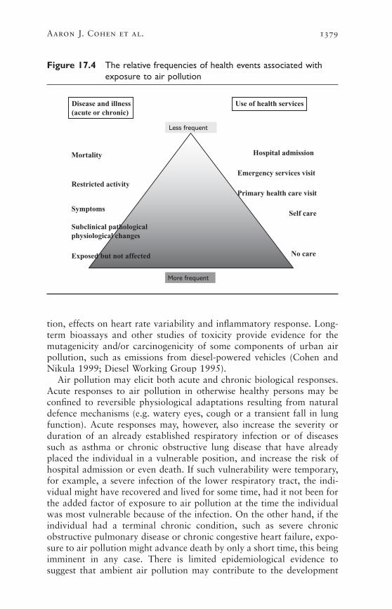
The past 10–15 years have seen a rapid increase in research on the healtheffects of air pollution, and it is now widely accepted that exposure tourban air pollution is associated with a broad range of acute and chronichealth effects, ranging from minor physiological disturbances to deathfrom respiratory and cardiovascular disease (Anonymous 1996a, 1996b;Figure 17.4). Recently, a committee of the American Thoracic Societyidentified effects on respiratory health associated with air pollution,which should be considered adverse, spanning outcomes from deathfrom respiratory diseases to reduced quality of life, and included someirreversible changes in physiological function (American ThoracicSociety 2000). In general, the frequency of occurrence of the healthoutcome is inversely related to its severity, with the consequence thatassessing total health impact solely in terms of the most severe, but lesscommon, outcomes, such as mortality, will underestimate the total healthburden of air pollution (WHO 2001b).
A large body of epidemiological research, discussed in more detailbelow, provides evidence that exposure to air pollution is associated withincreased mortality and morbidity. The respiratory and cardiovascularsystems appear to be the most affected. A growing body of toxicologi-cal and clinical evidence currently offers some limited insight into themechanisms through which exposure to air pollution may produce theeffects on respiratory and cardiovascular outcomes observed in epi-demiological studies (Anonymous 1996a, 1996b; Health Effects Institute2002). These mechanisms may involve decrements in pulmonary func-
1378 Comparative Quantification of Health Risks
tion, effects on heart rate variability and inflammatory response. Long-term bioassays and other studies of toxicity provide evidence for themutagenicity and/or carcinogenicity of some components of urban airpollution, such as emissions from diesel-powered vehicles (Cohen andNikula 1999; Diesel Working Group 1995).
Air pollution may elicit both acute and chronic biological responses.Acute responses to air pollution in otherwise healthy persons may beconfined to reversible physiological adaptations resulting from naturaldefence mechanisms (e.g. watery eyes, cough or a transient fall in lungfunction). Acute responses may, however, also increase the severity orduration of an already established respiratory infection or of diseasessuch as asthma or chronic obstructive lung disease that have alreadyplaced the individual in a vulnerable position, and increase the risk ofhospital admission or even death. If such vulnerability were temporary,for example, a severe infection of the lower respiratory tract, the indi-vidual might have recovered and lived for some time, had it not been forthe added factor of exposure to air pollution at the time the individualwas most vulnerable because of the infection. On the other hand, if theindividual had a terminal chronic condition, such as severe chronicobstructive pulmonary disease or chronic congestive heart failure, expo-sure to air pollution might advance death by only a short time, this beingimminent in any case. There is limited epidemiological evidence tosuggest that ambient air pollution may contribute to the development
Aaron J. Cohen et al. 1379
Figure 17.4 The relative frequencies of health events associated withexposure to air pollution
Mortality
Restricted activity
Subclinical pathologicalphysiological changes
Exposed but not affected
Hospital admission
Emergency services visit
Primary health care visit
Self care
No care
Symptoms
Use of health servicesDisease and illness(acute or chronic)
Less frequent
More frequent
of diseases such as chronic obstructive pulmonary disease, for whichsmoking and, in developing countries, indoor air pollution, are also riskfactors (Abbey et al. 1999; Pope and Dockery 1999; Tager et al. 1998).Distributions of short-and long-term vulnerability, reflecting the preva-lence of acute and chronic cardiorespiratory disease, may well differacross populations worldwide. This will have implications for the trans-ferability of risk functions from studies in populations in NAWE to populations where differences in genetic factors, diet, tobacco smoking,extent of urbanization, distribution of wealth and other factors relatedto social class, have resulted in different patterns of disease.
For example, recent analyses of two cohorts in the United States(Krewski et al. 2000) showed clearly that the effects of long-term expo-sure to air pollution on mortality depend on attained educational level,with the largest relative effects observed among the least educated.Recent studies in developing countries have also reported such gradientsin the relative risks of mortality (O’Neill et al. 2003). It is not clear whatfactor(s) might be responsible for these observations (e.g. aspects of occupation or diet), but it is reasonable to expect that they might varyacross the globe. Differences in vulnerability to air pollution introducea source of uncertainty in our estimates that can currently be only par-tially quantified.
Epidemiological evidence about exposure–response relationships ismost directly applicable to the risk assessment of air pollution, becauseit comes from the direct observation of human populations under rele-vant conditions (Samet 1999). Epidemiological studies have limitationsthat are largely a result of their observational nature. These relate to theaccurate measurement of exposure, definition of outcomes and inter-pretation of associations that are observed. Assessing the causality ofsuch associations requires a process of scientific reasoning that considersall evidence, including that from experimental studies (WHO 2000b).While there remain many gaps in our knowledge about the explanationsfor epidemiological associations, they can provide the best evidence toguide action to reduce the exposure of the population to air pollution,and to undertake health impact assessments, provided the uncertaintiesare recognized.
The epidemiology of air pollution takes advantage of the fact that con-centrations of urban air pollution, and thus human exposure, vary inboth time and space. For the most part, current epidemiological researchhas focused on either one or the other dimension, but infrequently onboth within the same population(s). Short-term temporal variation inconcentrations of air pollution over days and weeks has been used toestimate effects on daily mortality and morbidity. Spatial variation inlong-term average concentrations of air pollution has provided the basisfor cross-sectional and cohort studies of long-term exposure.
1380 Comparative Quantification of Health Risks

3.1 Studies of short-term exposure
The effects of short-term exposure to air pollution have been extensivelystudied in time-series studies in which daily rates of health events (e.g.deaths or hospital admissions) in one or more locales are analysed inrelation to contemporaneous series of daily concentrations of air pollu-tants, and other risk factors (e.g. weather) that vary over time periodsof months or years. Regression techniques are used to estimate a coeffi-cient that represents the relationship between exposure to pollution andthe outcome variable. The usual method of regression models the loga-rithm of the outcome, and thus arrives at an estimate of the relative risk,a proportional change in the outcome per increment of ambient con-centration. There has been a rapid increase in the number of these studiesas computing and statistical techniques have improved and as data onoutcomes and air pollution have become more extensive and easily acces-sible from routine sources. It is a strength of these studies that individ-ual cofactors, such as smoking, nutrition, behaviour, genetic factors, etc.,are unlikely confounders because they are not generally associated, on aday-to-day basis, with the daily concentration of air pollution. Studiesof time series have found associations between concentrations of PM inthe air and a large range of outcomes. These have been reviewed by Popeand Dockery (1999) and include daily mortality (all causes, respiratory,cardiovascular), hospitalization for respiratory diseases (all causes,chronic obstructive pulmonary disease, asthma, pneumonia) and for cardiovascular diseases (acute myocardial infarction, congestive cardiacfailure). Since this review, associations have also been reported forprimary health care visits for disease of the lower respiratory tract, anddiseases of the upper respiratory tract of both infective and allergic origin(Hajat et al. 2001, 2002). However, recent methodological studies andre-examination of earlier work indicate that the magnitude of the esti-mates of relative risk from time-series studies of daily mortality dependson the approach used to model both the temporal pattern of exposure(Braga et al. 2001) and potential confounders that vary with time, suchas season and weather (Health Effects Institute 2003).
The acute effects of air pollution have also been studied longitudinallyin panel studies, which can provide evidence of physiological effects atan individual level. Small groups, or panels, of individuals are followedover short time intervals, and health outcomes, exposure to air pollutionand potential confounders are ascertained for each subject on one ormore occasions. Panel studies have generally reported associations ofexposure to urban air pollution with increased prevalence of symptomsinvolving the upper and lower respiratory tract, and increased rates ofasthma attacks and medication use. Associations with short-term reduc-tion in lung function and the prevalence of cough symptoms have beenreported in studies in the United States (Pope and Dockery 1999), but are not consistently supported by studies in Europe (Roemer et al.1999).
Aaron J. Cohen et al. 1381

TIME-SERIES STUDIES IN ADULTS ACROSS THE WORLD
Studies of time series concerning daily mortality and, to a lesser extent,daily hospital admissions, have been conducted in cities throughout the world. A recent meta-analysis summarized the evidence from >100studies of daily mortality (Stieb et al. 2003). In addition, large studieshave now been conducted using uniform methods for assembling andanalysing data from multiple cities: APHEA 2 (Air Pollution and Health:A European Approach) (Katsouyanni et al. 1996, 2001) and NMMAPS(National Mortality and Morbidity Air Pollution Study) (Health EffectsInstitute 2000a, 2000b) in the United States. These multi-city studieshave confirmed the findings of earlier studies of individual cities infinding positive associations between daily mortality and hospital admis-sions and concentrations of PM, and have also attempted to explain theheterogeneity among cities in the relative risks associated with exposureto air pollution. For example, in the APHEA 2 Study, it was found thatthe effects of PM on mortality were modified by mean concentrations ofnitrogen dioxide (Katsouyanni et al. 2001), and in the NMMAPS Study,daily mortality was modified by the long-term average concentrations ofPM10. Levy et al. (2000) reported that the effects of PM10 were greaterin cities where PM2.5 comprised a higher proportion of PM10.
Most studies of time series are from countries in NAWE, where airpollution is low and decreasing and populations are characterized bywestern lifestyles and patterns of disease. To examine the epidemiologi-cal evidence for other non-NAWE countries, we searched a database ofstudies of time series and panel studies compiled at St George’s Hospi-tal Medical School, for which researchers had systematically ascertained,reviewed, and abstracted results from studies published in the peer-reviewed scientific literature (WHO 2003). All studies meeting pre-specified quality criteria related to adequacy of confounder control, andwhich provided estimates of the concentration–response relationship andits statistical precision were included. We classified them by the sub-region in which the study was performed and tabulated the results forsix outcomes: all-cause mortality, respiratory mortality, cardiovascularmortality, infant and child mortality, reduction in peak expiratory flowrate and cough symptom.
The distribution of time-series and panel studies by outcome and sub-region is shown in Tables 17.5(a) and (b). Up to mid-November 2001,the number of studies from AMR-A (71) and EUR-A (75) far exceededthe total for the remaining 12 subregions (42). The next largest con-tributor was AMR-B (Central and South America), with 18 studies. Thetable shows the numbers of panel studies presenting usable numericalestimates. Only 14 studies from non-NAWE subregions were identified,compared with 64 from the NAWE subregions. Some of the non-NAWEcountries had lifestyles and patterns of disease similar to those inNAWE—those in Australasia, for example.
1382 Comparative Quantification of Health Risks

Aaron J. Cohen et al. 1383
Table 17.5 Distribution of studies by outcome status and subregion
(a) Selected time-series studies
Outcome status
Cause of mortalityHospital
admissions/ Other TotalAll Respiratory Cardiovascular emergency time-series (from
Subregion causes disease disease room visits studies subregion)
AFR-D 0 0 0 0 0 0
AFR-E 0 0 0 0 0 0
AMR-A 34 11 13 39 2 71
AMR-B 10 9 6 5 0 18
AMR-D 0 0 0 0 0 0
EMR-B 0 0 0 0 0 0
EMR-D 0 0 0 0 0 0
EUR-A 44 28 24 28 3 75
EUR-B 4 3 4 0 0 5
EUR-C 0 0 0 0 0 0
SEAR-B 1 1 1 0 0 1
SEAR-D 0 0 0 0 0 0
WPR-A 4 4 4 2 0 6
WPR-B 8 3 4 4 0 12
World (from 113 78 5 187outcome status)
(b) Selected panel studies
Outcome status for valid studies Total for selected studiesSubregion Lung function Symptoms (from subregion)
AFR-D 0 0 0
AFR-E 0 0 0
AMR-A 19 17 28
AMR-B 3 3 3
AMR-D 0 0 0
EMR-B 0 0 0
EMR-D 0 0 0
EUR-A 32 31 38
EUR-B 3 2 3
EUR-C 2 1 2
SEAR-B 0 0 0
SEAR-D 0 1 1
WPR-A 4 1 4
WPR-B 0 1 1
World (from 62 57 79outcome status)

1384 Comparative Quantification of Health Risks
Figures 17.5 and 17.6 show the results for daily mortality and PM,by subregion, for adults and children, respectively. These estimates werescaled to PM10 (PM2.5 =0.6xPM10, BS=0.5xPM10, TSP=2xPM10). Thesescaling factors were decided after examining a number of co-locatedmeasures, but are likely to be variable across the individual cities. Esti-mates of random effects and fixed effects are shown because there is heterogeneity.
The pooled estimates are shown in Table 17.6. Most of the studies ofmortality showed relative risks of >1.0 (i.e. a change of >0.0%), withlower 95% confidence intervals also >1.0. However, the studies showingthe largest confidence intervals also tended to have the largest effects,this indicating the possibility of publication bias. There was considerableheterogeneity in the estimates. For this reason, the summary estimate forrandom effects is more appropriate because it takes into account thegreater uncertainty. The estimate for random effects was increased andstatistically significant for mortality from all causes, respiratory and car-diovascular diseases. It is remarkable that for daily mortality, the pooledestimate for the non-NAWE subregions of 0.5% increase in daily mor-tality per 10mg/m3 increase in PM was very similar to the estimates produced by the APHEA 2 and NMMAPS studies of 0.6 and 0.5, respec-tively. A recent meta-analysis of 109 published studies from around theworld reports similar estimates (Stieb et al. 2003).
These results indicate that daily mortality is positively associated withshort-term exposure to urban air pollution at time-scales in the order ofdays, in all subregions where this association has been measured. Theyalso suggest that the relative effect of exposure may also be of similarmagnitude in different parts of the world.
AIR POLLUTION AND REPRODUCTIVE AND CHILD HEALTH
Six time-series studies of daily mortality report associations between par-ticulate pollution and adverse effects in children, and all of them are fromnon-NAWE countries. Their estimates are shown in Figure 17.6. Fourwere from São Paulo (Conceiao et al. 2001; Gouveia and Fletcher 2000;Pereira et al. 1998; Saldiva et al. 1994), one from Mexico City (Loomiset al. 1999) and one from Bangkok (Ostro et al. 1999a). The Bangkokstudy was of PM10 and daily mortality from all causes in children aged<6 years. The study conducted in Mexico City evaluated the impact ofdaily changes in concentrations of PM2.5 and total mortality in childrenaged <1 year. Three studies in São Paulo (Conceiao et al. 2001; Gouveiaand Fletcher 2000; Saldiva et al. 1994), conducted during differentperiods of time, all reported an association between PM and mortalityfrom respiratory disease in children aged <5 years. The study conductedin São Paulo by Pereira et al. (1998) investigated the association of expo-sure to urban air pollution with intrauterine mortality. Some of the rel-ative risks reported in these studies were >1.0, but only the estimate fromMexico City was statistically significant at the 95% level.

Aaron J. Cohen et al. 1385F
igur
e 17
.5Pe
rcen
tage
cha
nge
in m
ean
daily
num
ber
of n
on-a
ccid
enta
l dea
ths,
in a
dults
,per
10
mg/m
3in
crea
se in
PM
10,
by c
ity
Not
e:Sc
alin
g fa
ctor
s us
ed:P
M2.
5=
0.6
¥PM
10,B
S=
0.5
¥PM
10,T
SP=
2¥
PM10
.
–2.0
–1.00.0
1.0
2.0
3.0
4.0
5.0
Mex
ico C
ity (L
oom
is et
al. 1
999)
Mex
ico C
ity (B
orja-
Aburto
et a
l. 199
8)
Mex
ico C
ity (B
orja-
Aburto
et a
l. 199
7)
Mex
ico C
ity (L
oom
is et
al. 1
996)
Santia
go (O
stro
et a
l. 199
6)
São P
aulo
(Sald
iva e
t al. 1
995)
Santia
go (S
anhu
eza
et a
l. 199
9)
Mex
ico C
ity (C
astill
ejos e
t al. 2
000)
Santia
go (C
ifuen
tes e
t al. 2
000)
São P
aulo
(Gou
veia
and
Fletch
er 2
000)
Lodz
(Wojt
yniak
and
Piek
arsk
a 19
96)
Pozna
n (W
ojtyn
iak a
nd P
iekar
ska
1996
)
Krako
w (Wojt
yniak
and
Piek
arsk
a 19
96)
Wro
claw (W
ojtyn
iak a
nd P
iekar
ska
1996
)
Bratis
lava
(Bac
haro
va e
t al. 1
996)
Krako
w (Krz
yzan
owsk
i and
Wojt
yniak
199
1)
Krako
w (Sza
franie
c and
Tec
za 1
999)
Bangk
ok (O
stro
et a
l. 199
9a)
Melb
ourn
e (S
imps
on e
t al. 2
000)
Christ
chur
ch (H
ales e
t al. 2
000)
Ulsan
(Lee
et a
l. 199
9)
Seoul
(Lee
et a
l. 199
9)
Beijing
(Xu
et a
l. 199
4)
Beijing
(Gao
199
3)
Inch
on (H
ong
et a
l. 199
9)
Inch
on (H
ong
et a
l. 199
9)
Sheny
ang
(Xu
et a
l. 200
0)
7 Kor
ean
Cities (
Lee
et a
l. 200
0)
Hong
Kong
SAR (Won
g et
al. 2
001)
Fixed-
effe
cts
Rando
m-e
ffects
% change in mean daily number of deaths per 10 mg/m3 increase in
concentration of PM10
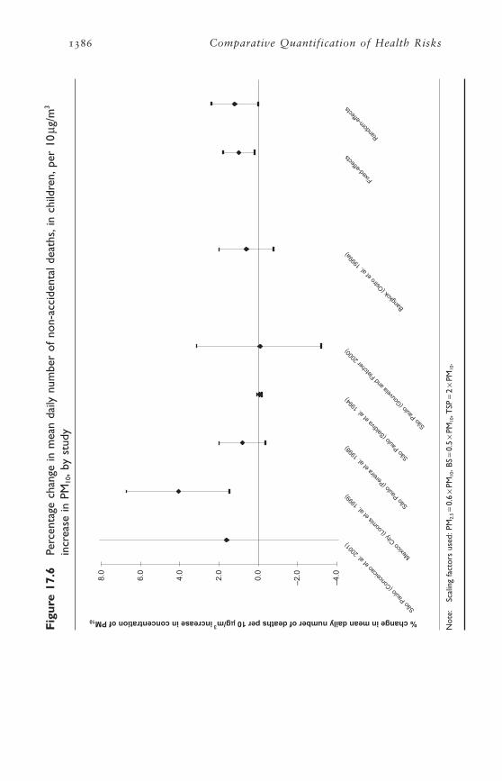
1386 Comparative Quantification of Health RisksF
igur
e 17
.6Pe
rcen
tage
cha
nge
in m
ean
daily
num
ber
of n
on-a
ccid
enta
l dea
ths,
in c
hild
ren,
per
10mg
/m3
incr
ease
in P
M10
,by
stud
y
Not
e:Sc
alin
g fa
ctor
s us
ed:P
M2.
5=
0.6
¥PM
10,B
S=
0.5
¥PM
10,T
SP=
2¥
PM10
.
–4.0
–2.00.0
2.0
4.0
6.0
8.0
São P
aulo
(Con
ceica
o et
al. 2
001)
Mex
ico C
ity (L
oom
is et
al. 1
999)
São P
aulo
(Per
eira
et a
l. 199
8)
São P
aulo
(Sald
iva e
t al. 1
994)
São P
aulo
(Gou
veia
and
Fletch
er 2
000)
Bangk
ok (O
stro
et a
l. 199
9a)
Fixed-
effe
cts
Rando
m-e
ffects
% change in mean daily number of deaths per 10 mg/m3 increase in concentration of PM10
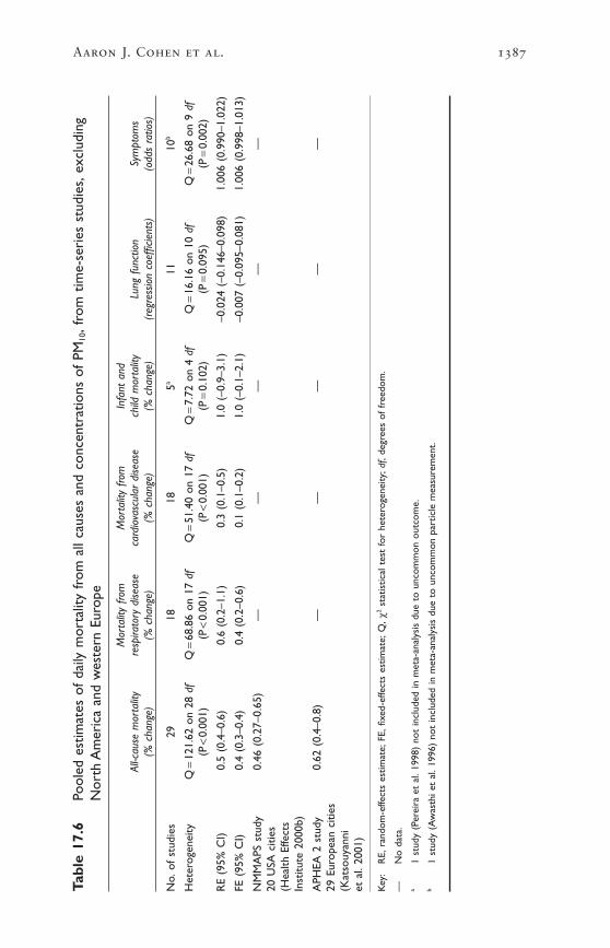
Aaron J. Cohen et al. 1387
Tabl
e 17
.6Po
oled
est
imat
es o
f da
ily m
orta
lity
from
all
caus
es a
nd c
once
ntra
tions
of
PM10
,fro
m t
ime-
seri
es s
tudi
es,e
xclu
ding
Nor
th A
mer
ica
and
wes
tern
Eur
ope
Mor
talit
y fro
m
Mor
talit
y fro
m
Infa
nt a
nd
All-c
ause
mor
talit
yre
spira
tory
dise
ase
card
iova
scul
ar d
iseas
ech
ild m
orta
lity
Lung
fun
ctio
nSy
mpt
oms
(% c
hang
e)(%
cha
nge)
(% c
hang
e)(%
cha
nge)
(reg
ress
ion
coef
ficie
nts)
(odd
s ra
tios)
No.
of s
tudi
es29
1818
5a11
10b
Het
erog
enei
tyQ
=12
1.62
on
28 d
fQ
=68
.86
on 1
7 df
Q=
51.4
0 on
17
dfQ
=7.
72 o
n 4
dfQ
=16
.16
on 1
0 df
Q=
26.6
8 on
9 d
f(P
<0.
001)
(P<
0.00
1)(P
<0.
001)
(P=
0.10
2)(P
=0.
095)
(P=
0.00
2)
RE
(95%
CI)
0.5
(0.4
–0.6
)0.
6 (0
.2–1
.1)
0.3
(0.1
–0.5
)1.
0 (–
0.9–
3.1)
–0.0
24 (
–0.1
46–0
.098
)1.
006
(0.9
90–1
.022
)
FE (
95%
CI)
0.4
(0.3
–0.4
)0.
4 (0
.2–0
.6)
0.1
(0.1
–0.2
)1.
0 (–
0.1–
2.1)
–0.0
07 (
–0.0
95–0
.081
)1.
006
(0.9
98–1
.013
)
NM
MA
PS s
tudy
0.46
(0.
27–0
.65)
——
——
—20
USA
citi
es(H
ealth
Effe
cts
Inst
itute
200
0b)
APH
EA 2
stu
dy0.
62 (
0.4–
0.8)
——
——
—29
Eur
opea
n ci
ties
(Kat
souy
anni
et
al.
2001
)
Key
:R
E,ra
ndom
-effe
cts
estim
ate;
FE,fi
xed-
effe
cts
estim
ate;
Q,c
2st
atis
tical
tes
t fo
r he
tero
gene
ity;d
f,de
gree
s of
fre
edom
.
—N
o da
ta.
a1
stud
y (P
erei
ra e
t al
.199
8) n
ot in
clud
ed in
met
a-an
alys
is d
ue t
o un
com
mon
out
com
e.b
1 st
udy
(Aw
asth
i et
al.1
996)
not
incl
uded
in m
eta-
anal
ysis
due
to
unco
mm
on p
artic
le m
easu
rem
ent.

Infant mortality from respiratory disease and other adverse perinatalevents, such as low birth weight and malformations, have also been asso-ciated with more prolonged exposure to air pollution (Bobak and Leon1999; Wilhelm and Ritz 2003; Woodruff et al. 1997). Woodruff et al.followed a large birth cohort in the United States for one year and esti-mated the relative risk of mortality associated with residential exposureto PM10 in the first two post-natal months, conditional on a variety ofpotential confounders, including maternal smoking. They reported anincrease in total mortality of 4% per 10mg/m3, and 20% for mortalityfrom respiratory causes. Two studies recently evaluated changes in infantmortality associated with reductions in industrial emissions caused by arecession and mandated reductions in pollution resulting from the UnitedStates Clean Air Act Amendments of 1970 (Chay and Greenstone 1999,2001). Using county-level data, the authors estimated that 4–8 infantdeaths per 100000 live births were prevented for each 1mg/m3 reductionin TSP.
STUDIES OF ACUTE MORBIDITY
Far fewer studies have been conducted of the association of exposure to urban air pollution with acute morbidity, especially in non-NAWEcountries. There were insufficient studies in any one outcome group to allow formal meta-analysis of non-NAWE studies, but most reports sug-gested a positive association with urban air pollution, consistent withthat observed in NAWE countries, especially for hospital admissions(Atkinson et al. 2001; Burnett et al. 1999; Health Effects Institute2000b). A recent study compared directly the effects of air pollution onhospital admissions in China, Hong Kong Special Administrative Region(Hong Kong SAR) and London. Similar associations were observed forPM10 and gaseous pollutants and hospital admissions for ischaemic heartdisease in both locations, and the associations were strongest duringseasons of low humidity in both cities, but no association with admis-sions for cardiac disease was observed in Hong Kong SAR (Wong et al.2002).
3.2 Studies of long-term exposure
COHORT STUDIES OF MORTALITY FROM CHRONIC RESPIRATORY AND
CARDIOVASCULAR DISEASE
Cohort studies take advantage of spatial heterogeneity in concentrationsof air pollution to compare the incidence of disease and death in popu-lations exposed in the long term to differing levels of pollution. By fol-lowing large populations for a number of years, cohort studies provideestimates of both attributable numbers of deaths and, more importantly,average reductions in life span attributable to air pollution.
The evidence from cohort studies of populations in Europe and theUnited States indicates that long-term exposure to urban air pollution
1388 Comparative Quantification of Health Risks

is associated with an increase in total and cardiopulmonary mortality in adults (Dockery et al. 1993; Hoek et al. 2002; Lipfert et al. 2003;McDonnell et al. 2000; Pope et al. 2002). In each of these studies, theeffects of potential confounders such as cigarette smoking, occupationand prior medical history were adjusted for in regression analyses. Moststudies find the strongest and most consistent associations with exposureto PM, and PM2.5 appears to be more closely associated with mortalitythan PM10 or TSP (Dockery et al. 1993; Pope et al. 2002). The recentlypublished results of a study conducted in the Netherlands confirm theimpacts of long-term exposure to air pollution, and in particular thatrelated to road traffic, on mortality (Hoek et al. 2002).
Unfortunately, the cohort studies provide little information on whenexposure to air pollution acts to increase the risk of mortality (i.e. theinduction time for mortality attributable to exposure to long-term expo-sure to air pollution), making it difficult to estimate when the effects ofreduction of air pollution might be observed.
Comparable cohort studies have not yet been carried out in develop-ing countries. However, the imposition of restrictions on the sulfurcontent of fuel for power generation and transportation in Hong KongSAR, instituted over short time intervals in 1990, provided opportuni-ties for researchers to measure directly the impact of reducing air pollu-tion on long-term average mortality (Hedley et al. 2002). Hedley et al.(2002) documented both changes in ambient air quality subsequent tothe imposition of the restrictions, and declines in long-term average ratesof mortality from cardiovascular and respiratory diseases associated withthose changes. Comparison of changes in mortality in more and less polluted areas of Hong Kong SAR provided limited ability to accountfor secular changes in other risk factors for mortality that could haveproduced the observed decrease in mortality following the change in thesulfur content of fuel. A similar study was also published recently byClancy et al. (2002), who measured decreased long-term average mor-tality in Dublin after the banning of the sale of bituminous coal in Dublinin 1990.
The American Cancer Society study
The American Cancer Society (ACS) study (Pope et al. 2002) in theUnited States is by far the largest cohort study of air pollution and long-term average mortality to date. The ACS study of air pollution and mortality is based in the ACS Cancer Prevention II Study, an on-goingprospective cohort of approximately 1.2 million adults from all 50 states(Calle et al. 2002). Friends and neighbours recruited cohort members onbehalf of the ACS. Participants were enrolled in 1982, when they wereaged ≥30 years, and their mortality has been ascertained through to1998. Data on a wide range of risk factors for cancer and other chronicdiseases were obtained from each participant. The ACS study links thedata for approximately 500000 cohort members with data on air pol-
Aaron J. Cohen et al. 1389

lution from metropolitan areas throughout the United States. The firststudy of air pollution and mortality in this cohort (Pope et al. 1995) wasbased on follow-up through to 1990. That study reported increases inmortality from cardiopulmonary disease for 19.9mg/m3 fine particulatesulfate (relative risk of 1.26, 95% CI 1.16–1.37), and from lung cancer(relative risk of 1.36, 95% CI 1.11–1.66). These findings were subse-quently corroborated in an independent re-analysis (Krewski et al. 2000).A more recent analysis of this cohort extended follow-up through to1998, and ascertained 40706 deaths from cardiopulmonary disease, and10749 from lung cancer. Data were analysed using Cox proportionalhazards regression models that incorporated both random effects andnon-parametric spatial smoothing to adjust for unmeasured factors cor-related spatially with air pollution and mortality across the United States.The models also adjusted for age, sex, race, education, marital status,body mass, diet, alcohol consumption, occupational exposures and theduration and intensity of cigarette smoking, all measured via question-naire at enrolment.
Concentrations of ambient air pollution had, in general, declinedacross the United States between 1982 and 1998. Measurements ofambient concentrations of fine particulate air pollution (PM2.5) in thecities where subjects resided at enrolment were available for periods bothbriefly preceding enrolment (1979–83) and immediately after follow-up(1999–2000). In separate regression analyses, cohort members wereassigned estimates of exposure corresponding to their city-of-residence-specific value for each of those periods, as well as for the average valueacross the two periods. For a change of 10mg/m3 in the ambient con-centration of PM2.5, the smallest relative increases were observed for themean concentration of the time period 1979–1983. This estimate wasbased on data from 61 cities, with a mean concentration of PM2.5 of 21.1mg/m3, and a range of 10–30mg/m3. The relative risks for a 10mg/m3
change in the concentration of ambient PM2.5 were larger when expo-sure was specified as the average of the ambient concentrations of thetwo time periods. This may be explained by the fact that the estimatesfrom the earliest periods are more subject to random (and non-differential) error. However, it also suggests that more recent exposuresmay be exerting the strongest effects on mortality, an interpretation alsooffered in the recent re-analysis of the earlier follow-up of the ACScohort (Krewski et al. 2000). Unfortunately, it was not possible to deriveindividual time-varying estimates of exposure from the available data(e.g. detailed residence histories were unavailable), precluding directevaluation of the induction time for mortality attributable to exposureto air pollution.
Long-term exposure and the incidence of chronic disease
Little evidence is available concerning exposure to air pollution and theincidence of chronic cardiovascular or respiratory disease. One study in
1390 Comparative Quantification of Health Risks

the United States reported an association of long-term exposure to PM10
with the incidence of self-reported physician-diagnosed chronic bron-chitis (Abbey et al. 1999). A recent case–control study reported an asso-ciation between short-term exposure and the incidence of non-fatalmyocardial infarction (Peters et al. 2001). Cross-sectional studies havefound associations with reduced lung function and increased respiratorysymptoms in both adults and children, which might in part representchronic disease as the result of long-term exposure. Several recent cross-sectional studies in large Chinese cities have reported increased preva-lence of respiratory symptoms in adults (Qian et al. 2001; Zhang et al.1999) and elementary school children (Qian et al. 2000; Zhang et al.2002) exposed to urban air pollution. A cross-sectional study in Delhiobserved reductions in pulmonary function in residents of highly pol-luted areas, but little evidence of increased prevalence of symptoms(Chhabra et al. 2001).
AIR POLLUTION AND LUNG CANCER
Epidemiological studies over the last 40 years have observed that generalambient air pollution, chiefly composed of the by-products of the incom-plete combustion of fossil fuels, is associated with small relative increasesin the incidence of lung cancer. The evidence derives from studies oftrends in the incidence of lung cancer, studies of occupational groups,comparisons of urban and rural populations, and case–control andcohort studies using diverse exposure metrics. Recent prospective cohortand case–control studies which have controlled for the effects of ciga-rette smoking, occupation and other risk factors have consistentlyobserved small increases in the relative risk of lung cancer in relation toexposure to particulate air pollution (Abbey et al. 1999; Dockery et al.1993; Krewski et al. 2000; Pope et al. 2002; Samet and Cohen 1999).A recent Swedish case–control study reported that excess lung cancerwas related specifically to exposure to mobile sources of air pollution,with the largest effects observed for exposure occurring 20 years priorto diagnosis (Nyberg et al. 2000).
3.3 Choice of outcomes and hazards
STUDIES USED FOR HAZARD ESTIMATES
The use of results from time series to estimate the disease burden attrib-utable to urban air pollution is problematic for various reasons. First,data on rates of occurrence, such as hospital admissions, primary healthcare consultations or asthma exacerbation are not collected in manycountries. Thus there is no baseline upon which to develop an estimateof health impact. Mortality is an exception in that data are availablefrom death registration or indirect demographic methods in all subregions.
Aaron J. Cohen et al. 1391

The application of the time-series concentration–response functions tothe assessment of mortality impact, however, is limited. Specifically, it isnot possible to use the results of studies of time series to estimate YLLin adults. This is because time-series studies of daily mortality do not inthemselves allow the estimation of lost life time, but rather only allowestimation of the number of deaths that have been brought forward byan unspecified amount of time. Recent research has made clear that thetime-series estimates reflect deaths that may have been brought forwardby as much as several months, rather than simply advancing the time ofdeath in frail people by a few days (Schwartz 2000; Zeger et al. 1999).The design of the time-series study of daily mortality, which requires thecontrol of long-term variation in air pollution, precludes estimation ofgreater losses (Künzli et al. 2001; Leksell and Rabl 2001; McMichael etal. 1998). Thus, the time-series studies only provide an estimate of thedaily number of deaths brought-forward.
Cohort studies include not only people whose deaths were advancedby recent exposure to air pollution, but also those who died from chronicdisease caused by long-term exposure (COMEAP 1998; Künzli et al.2001), thus they provide a more comprehensive estimate of the effectson mortality. Furthermore, because their relative risks can be applied topopulation life tables, the effects of air pollution on life span can be esti-mated (Brunekreef 1997; COMEAP 2001; Hurley et al. 2000; Sommeret al. 2000)
The situation may be different for children. In developing countries,the major causes of death, such as acute respiratory disease, are verylikely to result from a severe acute infection, which represents a briefwindow of vulnerability. If the child survives, they might be expected tofully recover and enjoy a full life expectancy. If we assume that deathwas not otherwise imminent, then these deaths, on average, represent theloss of considerable life years. Under such an assumption, one could usetime-series estimates to estimate YLL in children aged 0–4 years.
In making these estimates, several further considerations should bekept in mind. The first is that the effects of cumulative exposure overseveral weeks are several times greater than those obtained by using asingle day lag and thus underestimate the impacts on health. The secondis that other air pollutants in the mixture may be exerting additionaleffects, may interact with particles or may be confounding the associa-tions of particles. Ozone, for example, is also toxic and while its effectstend to be independent of PM, it also seems to modify the effect of par-ticles on number of hospital admissions (Atkinson et al. 2001).
DEFINITION AND SPECIFICATION OF HEALTH OUTCOMES
We estimated the burden of disease imposed by mortality from car-diopulmonary disease and lung cancer in adults, and from ARI in chil-dren aged 0–4 years. We made this choice despite the fact, discussedabove, that other serious health effects of air pollution are well-
1392 Comparative Quantification of Health Risks

documented, and that still others appear from more limited evidence tobe of potential concern. Our decision to focus on mortality outcomeswas made on the basis of the following considerations.
• Strength of evidence. A large body of research from many parts of theworld indicates that ambient air pollution causes increased daily mor-tality from cardiovascular and respiratory disease. There appear to becomparable effects in the cities of developed and developing countries,on the basis of the limited evidence available. Although no cohortstudies of mortality have as yet been conducted in developing coun-tries, the possibility that associations comparable to those observedin the United States would be observed is strengthened by the resultsof the studies of daily mortality, and the limited results from studiesof morbidity.
• Consistent definition of the end-point. Mortality per se is a well-defined event that is registered in most countries. For this reason, epidemiologists have frequently measured the effect of air pollutionon total mortality from all natural causes, ascertained from death cer-tificates or other sources of vital statistics. Other outcomes, such asbronchitis and the symptom of wheeze, are subject to very large vari-ations in severity, and without such qualification their impact onhealth is difficult to assess. The definitions of other possible healthoutcomes, such as restricted activity days, use of primary health careservices, diagnoses and school absences, are likely to vary withnational culture and among health care systems.
The cause of death is more problematic because it is not certified medically in many countries, and there are considerable differencesbetween and within countries in terms of diagnostic practice. Never-theless, we propose to base our estimates primarily on cardiopul-monary, rather than total, mortality. There is strong evidence fromboth time-series and cohort studies that ambient air pollution specif-ically increases the risk of death from these causes. Moreover, varia-tions in the relative contribution of non-cardiopulmonary mortalityamong countries could increase the error in the burden assessment,particularly in countries with lower cardiopulmonary death rates,potentially leading to overestimates of impact. Since considerablecross-coding is likely, we have chosen to use the combined car-diopulmonary group consisting of GBD infectious and chronic respi-ratory diseases and selected cardiovascular outcomes for adults. Inchildren, death from cardiovascular diseases is rare and the pul-monary group is adequate.
• Availability of baseline occurrence rates. Data on age-specific mortal-ity are collected or estimated using consistent methods for all subre-gions. This is not the case for some important potential measures ofmorbidity, such as the frequency of asthma attacks, or measures of
Aaron J. Cohen et al. 1393
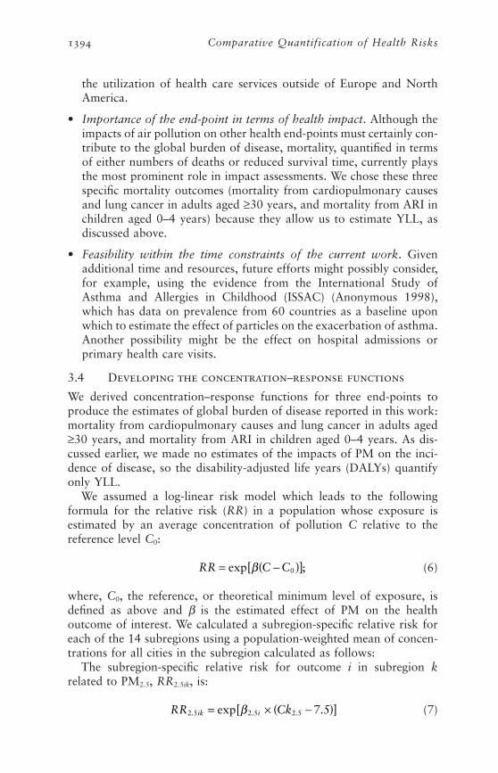
the utilization of health care services outside of Europe and NorthAmerica.
• Importance of the end-point in terms of health impact. Although theimpacts of air pollution on other health end-points must certainly con-tribute to the global burden of disease, mortality, quantified in termsof either numbers of deaths or reduced survival time, currently playsthe most prominent role in impact assessments. We chose these threespecific mortality outcomes (mortality from cardiopulmonary causesand lung cancer in adults aged ≥30 years, and mortality from ARI inchildren aged 0–4 years) because they allow us to estimate YLL, asdiscussed above.
• Feasibility within the time constraints of the current work. Givenadditional time and resources, future efforts might possibly consider,for example, using the evidence from the International Study ofAsthma and Allergies in Childhood (ISSAC) (Anonymous 1998),which has data on prevalence from 60 countries as a baseline uponwhich to estimate the effect of particles on the exacerbation of asthma.Another possibility might be the effect on hospital admissions orprimary health care visits.
3.4 Developing the concentration–response functions
We derived concentration–response functions for three end-points toproduce the estimates of global burden of disease reported in this work:mortality from cardiopulmonary causes and lung cancer in adults aged≥30 years, and mortality from ARI in children aged 0–4 years. As dis-cussed earlier, we made no estimates of the impacts of PM on the inci-dence of disease, so the disability-adjusted life years (DALYs) quantifyonly YLL.
We assumed a log-linear risk model which leads to the followingformula for the relative risk (RR) in a population whose exposure is estimated by an average concentration of pollution C relative to the reference level C0:
(6)
where, C0, the reference, or theoretical minimum level of exposure, isdefined as above and b is the estimated effect of PM on the healthoutcome of interest. We calculated a subregion-specific relative risk foreach of the 14 subregions using a population-weighted mean of concen-trations for all cities in the subregion calculated as follows:
The subregion-specific relative risk for outcome i in subregion krelated to PM2.5, RR2.5ik, is:
(7)RR Ckik i2 5 2 5 2 5 7 5. . .exp .= ¥ -( )[ ]b
RR C C= -( )[ ]exp ;b 0
1394 Comparative Quantification of Health Risks
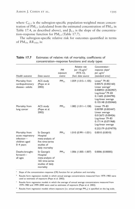
where Ck2.5 is the subregion-specific population-weighted mean concen-tration of PM2.5 (calculated from the estimated concentration of PM10 inTable 17.4, as described above), and b2.5i is the slope of the concentra-tion–response function for PM2.5 (Table 17.7).
The subregion-specific relative risk for outcomes quantified in termsof PM10, RR10ik, is:
Aaron J. Cohen et al. 1395
Table 17.7 Estimates of relative risk of mortality, coefficients ofconcentration–response functions and study types
Relative risk Concentration–PM per 10 mg/m3 response slopea
exposure (95% CI), per mg/m3
Health outcome Data source metric from data source (standard error)
Mortality from ACS study PM2.5 1.059 (1.015–1.105) Linearb 79–83cardiopulmonary (Pope et al. 0.00575 (0.002160)disease—adults 2002) Linear averagec
0.008933 (0.002907)Log-lineard 79–830.11605 (0.044790)Log-linear average0.155148 (0.050460)
Mortality from ACS study PM2.5 1.082 (1.011–1.158) Linear 79–83lung cancer (Pope et al. 0.00789 (0.003447)
2002) Linear average0.012673 (0.00426)Log-linear 79–830.17114 (0.071968)Log-linear average
0.232179 (0.074770)
Mortality from St George’s PM10 1.010 (0.991–1.031) 0.0010 (0.0010)acute respiratory Hospital infection— meta-analysis of children aged five time-series 0–4 years studies of
daily mortality
Deaths-brought- St George’s PM10 1.006 (1.005–1.007) 0.0006 (0.00005)forward— Hospital all ages meta-analysis of
165 time-series studies of daily mortality
a Slope of the concentration–response (CR) function for air pollution and mortality.b Results form regression models in which annual average concentrations measured from 1979–1983 were
used as estimates of exposure (Pope et al. 2002).c Results form regression models in which the average of annual average concentrations measured from
1979–1983 and 1999–2000 were used as estimates of exposure (Pope et al. 2002).d Results from regression models where exposure (i.e. annual average PM2.5) is specified on the log scale.

1396 Comparative Quantification of Health Risks
(8)
where Ck10 is the subregion-specific population-weighted mean concen-tration of PM10 (Table 17.4), and b10i is the slope of the concentra-tion–response function for PM10. The city-specific concentrations ofPM10 were truncated at 15 and 100mg/m3 for calculation of subregion-specific population-weighted mean concentrations of PM10.
MORTALITY FROM CARDIOPULMONARY DISEASE AND LUNG CANCER
IN ADULTS
We used the results of the ACS study of urban air pollution and mor-tality (Pope et al. 2002) to estimate attributable deaths and YLL fromcardiopulmonary diseases and lung cancer in adults aged ≥30 years. In our base-case analyses we used the estimates of the concentration–response functions based on the ambient concentrations in 1979–1983,which correspond to increases of 5.9% and 8.2% in mortality from car-diopulmonary disease and lung cancer, respectively, for each 10mg/m3
change in the ambient concentration of PM2.5 (Table 17.7).Deaths from cardiopulmonary disease and lung cancer in the ACS
cohort were defined as persons whose underlying cause of death was coded according to the International Statistical Classification of Diseases, ninth revision, on their death certificates as ICD-9 401–440and 460–519, and 162, respectively. When calculating the attributablefraction, ACS concentration–response functions for cardiopulmonarydisease defined in this way were applied to baseline cause-specific ratesof mortality in the GBD project. For lung cancer, this correspondedexactly to the definition used in the ACS study. For cardiopulmonarydeaths, the GBD groupings of cause of death (39, 40, 106–109, 111) didnot include several ICD codes (406–409, 415–417, 423–424, 426–429,440) that were included in the ACS definition. These codes representdiverse cardiac diseases, including conduction disorders, cardiac dys-rhythmias, heart failure and ill-defined cardiac causes. Together theycomprise approximately 18% of all cardiopulmonary deaths in the ACSstudy (R. Burnett, personal communication).
The ACS study estimated concentration–response functions for PM2.5
over a range that extends from annual average concentrations of PM2.5
of about 5–30mg/m3 (Pope et al. 2002). The shape of the concentra-tion–response function for fine particulate air pollution outside thatrange is currently unknown, as noted above, and estimated annualaverage concentrations of PM2.5 in some subregions are outside thatrange (Table 17.1). In our base-case analyses we limited the risk of mor-tality in any city to be no greater than that attained at a concentrationof PM2.5 of 50mg/m3 (Figure 17.7). Thus, for cities with estimated annualaverage concentrations of >50mg/m3, we assigned a maximum concen-tration, or Cm, equal to 50mg/m3, regardless of their actual estimated
RR Cik i k10 10 10 15= ¥ -( )[ ]exp b

concentration. This means that the excess risk is constrained to be nogreater than that associated with an annual average concentration of 50mg/m3, regardless of the actual estimated annual average concentra-tion. The counterfactual or theoretical minimum concentration was setat 7.5mg/m3, as discussed above.
We set the maximum city-specific concentration of PM2.5, Cm, at 50mg/m3 to avoid producing unrealistically large estimates of mortalityin the most extremely polluted subregions under a linear exposure model.With Cm =50, the subregion-specific attributable fraction was restrictedto no more than approximately 25% of the burden of a given healthoutcome, while not greatly exceeding the maximum observed annualaverage concentration in the ACS study. We also examined alternativevalues for the shape of the concentration–response function for PM2.5
and mortality from cardiopulmonary disease and lung cancer in sensi-tivity analyses, as described below.
MORTALITY FROM ACUTE RESPIRATORY INFECTIONS IN CHILDREN AGED
0–4 YEARS
In view of the importance of mortality from ARI among children indeveloping countries and the suggestion from available evidence of anassociation with air pollution (Romieu et al. 2002), we decided to make
Aaron J. Cohen et al. 1397
Figure 17.7 Alternative concentration–response curves for mortalityfrom cardiopulmonary disease, using different scenarios

a summary estimate on the basis of these studies, in spite of their het-erogeneity in outcomes and age groups.
To estimate the relationship between exposure to PM and mortalityfrom ARI among children aged 0–4 years, we computed a summary esti-mate from the five published time-series studies discussed above (Table17.6 and Figure 17.6). One study (Pereira et al. 1998) was excludedbecause the outcome, intrauterine mortality, was clearly unrelated toARI. The five remaining studies were summarized as a weighted averageof the estimates from individual studies (scaled to PM10, as discussedabove) with the weights determined by the inverse of the reported vari-ance in the concentration–response function. We estimate that a 10mg/m3
increase in ambient concentrations of PM10 results in a 1.0% (95% CI—0.9%–3.1%) increase in daily mortality from ARI in children aged 0–4years (Table 17.7).
When calculating the attributable fraction, this concentration–response function was applied to GBD baseline cause-specific rates ofmortality from acute respiratory infection (GBD code 38) that includesICD-9 codes 460–466, 480–487 and 381–382.
NUMBERS OF DEATHS FROM ALL NATURAL CAUSES CAUSED BY SHORT-TERM
EXPOSURE TO URBAN AIR POLLUTION IN ADULTS
We also calculated an estimate of the numbers of deaths from all natural(non-injury) causes attributable to short-term exposure to urban air pol-lution using an estimate of concentration–response derived from inter-national literature on air pollution and daily mortality. This estimate wasnot included in the total attributable deaths and disease burden becauseof the conceptual issue in quantifying the effects of short-term exposurediscussed above.
Using the St George’s Hospital Medical School database, describedabove, we identified 165 time-series studies of PM10 and daily mortalityfrom all causes at all ages in all languages and countries, up to the endof July 2001. As we were concerned about the possibility of publicationbias, we compared the summary estimates from 54 individual studies, a subset of the literature which would be expected to be susceptible topublication bias, with those of the two multi-city studies (Health Effects Institute 2000b; Katsouyanni et al. 2001), which selected citiesfrom a pre-specified sampling frame, used uniform methods of analysis,and published all results. The pooled estimate for the cities of the combined APHEA and NMMAPS studies (n=111) was 1.005 (95% CI1.004–1.006) with no evidence of publication bias in the funnel plot oron statistical testing. For the 54 studies of individual cities, graphicalanalysis showed some evidence of publication bias but when formallytested, this was weak (P=0.12). The pooled estimate was 1.007 (95%CI 1.006–1.008) but when adjusted for publication bias using Trim andFill analysis, it was reduced to 1.006 (95% CI 1.004–1.007). We thenexamined the results for all 165 studies with results for PM10. There was
1398 Comparative Quantification of Health Risks
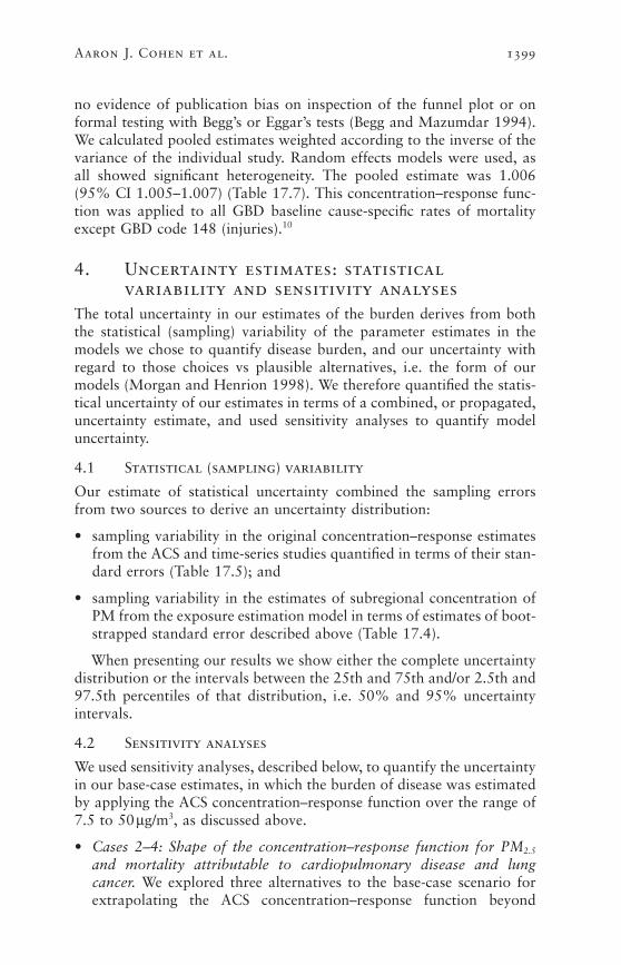
no evidence of publication bias on inspection of the funnel plot or onformal testing with Begg’s or Eggar’s tests (Begg and Mazumdar 1994).We calculated pooled estimates weighted according to the inverse of thevariance of the individual study. Random effects models were used, asall showed significant heterogeneity. The pooled estimate was 1.006(95% CI 1.005–1.007) (Table 17.7). This concentration–response func-tion was applied to all GBD baseline cause-specific rates of mortalityexcept GBD code 148 (injuries).10
4. Uncertainty estimates: statisticalvariability and sensitivity analyses
The total uncertainty in our estimates of the burden derives from boththe statistical (sampling) variability of the parameter estimates in themodels we chose to quantify disease burden, and our uncertainty withregard to those choices vs plausible alternatives, i.e. the form of ourmodels (Morgan and Henrion 1998). We therefore quantified the statis-tical uncertainty of our estimates in terms of a combined, or propagated,uncertainty estimate, and used sensitivity analyses to quantify modeluncertainty.
4.1 Statistical (sampling) variability
Our estimate of statistical uncertainty combined the sampling errorsfrom two sources to derive an uncertainty distribution:
• sampling variability in the original concentration–response estimatesfrom the ACS and time-series studies quantified in terms of their stan-dard errors (Table 17.5); and
• sampling variability in the estimates of subregional concentration ofPM from the exposure estimation model in terms of estimates of boot-strapped standard error described above (Table 17.4).
When presenting our results we show either the complete uncertaintydistribution or the intervals between the 25th and 75th and/or 2.5th and97.5th percentiles of that distribution, i.e. 50% and 95% uncertaintyintervals.
4.2 Sensitivity analyses
We used sensitivity analyses, described below, to quantify the uncertaintyin our base-case estimates, in which the burden of disease was estimatedby applying the ACS concentration–response function over the range of7.5 to 50mg/m3, as discussed above.
• Cases 2–4: Shape of the concentration–response function for PM2.5
and mortality attributable to cardiopulmonary disease and lungcancer. We explored three alternatives to the base-case scenario forextrapolating the ACS concentration–response function beyond
Aaron J. Cohen et al. 1399

30mg/m3, the highest annual average concentration observed in theACS study (Figure 17.7).
• Case 2: No incremental increase in excess mortality above 30mg/m3
PM2.5. Under this scenario, when calculating the population-weightedsubregional average concentration of PM2.5 we give the city-specificCm a value of 30mg/m3, regardless of the estimated concentration,rather than the base-case concentration of 50mg/m3. This means thatthe excess risk is constrained to be no greater than that associatedwith an annual average concentration of 30mg/m3, regardless of theactual estimated annual average concentration. The counterfactual ortheoretical minimum concentration was set at 7.5mg/m3. We consid-ered this the estimator that would produce the smallest (i.e. most sci-entifically conservative) estimate of the impact of mortality consistentwith the use of the ACS concentration–response function.
• Case 3: Excess mortality increases linearly above 30mg/m3 PM2.5.Under this scenario, the city-specific concentration of PM2.5 takes its actual estimated value when calculating the population-weightedsubregional averages, i.e. in contrast to the base-case and case 2scenarios. The counterfactual or theoretical minimum concentrationwas set at 7.5mg/m3. We considered this the estimator that wouldproduce the largest estimate of mortality impact consistent with theuse of the ACS concentration–response function.
• Case 4: Excess mortality increases with the log of concentration ofPM2.5 across the entire range. Under this scenario, the city-specificconcentration of PM2.5 takes the log of its actual estimated value whencalculating the population-weighted subregional averages. Therefore,in contrast to case 3, the slope of the concentration–response func-tion is constrained to decrease at higher concentrations. The coun-terfactual or theoretical minimum concentration was set at 7.5mg/m3.
We included this estimator, proposed by an external reviewer after wehad made our initial estimates (R. Burnett, personal communication),because it seemed a reasonable way to characterize an excess risk thatwe believed may: (i) increase directly with ambient levels over theentire range of annual average concentrations that we estimated forthe world’s cities, but (ii) be smaller at higher ambient concentrations,as has been observed for daily mortality in time-series studies (Danielset al. 2000; Schwartz et al. 2002).
• Cases 5 and 6: Choice of ACS concentration–response function. Inthe base-case analyses, we used the ACS coefficients that were basedon exposure of the cohort in 1979–1983. These arguably best repre-sented the effects of long-term past exposure that some researchersassume are responsible for the increased mortality attributable to airpollution in that cohort through to 1998. There is, however, consid-
1400 Comparative Quantification of Health Risks
erable uncertainty regarding the timing of exposure with regard torisk of mortality (Krewski et al. 2000), so we calculated alternativeestimates using the reported ACS coefficients based on the average ofpast (1979–1983) and recent (1999–2000) annual average concen-trations using both a linear (case 5) and log-linear (case 6) extrapo-lation (Table 17.7).
• Case 7: Change PM2.5 :PM10 ratio. In the base-case analyses, weassumed a PM2.5 :PM10 ratio of 0.50, although higher and lower ratioshave been observed in a number of locations, as discussed above. Weexamined the sensitivity of our base-case analyses by assigning citiesin AMR-A, EUR-A, EUR-B, EUR-C and WPR-A a higher scalingfactor of 0.65, while assigning a lower scaling factor of 0.35 to citiesin all other subregions.
• Cases 8 and 9: Choice of counterfactual or theoretical minimum concentration. We evaluated the sensitivity of the base-case estimatesto two different choices of counterfactual PM2.5 concentration: 3mg/m3 (case 8) and 15mg/m3 (case 9). The former is close to the minimum background level of PM2.5 observed in the United States, and the latter is the annual concentration of PM2.5 proposedby the United States National Ambient Air Quality Standard(NAAQS) (U.S. Environmental Protection Agency 2002). Each value was substituted for the base-case concentration of 7.5mg/m3 inEquation 7 above, when calculating population-weighted subregionalrelative risks.
5. Results
5.1 Base-case estimates
We estimated that exposure to particulate air pollution caused approxi-mately 800000 excess deaths and 6.4 million DALYs (consisting only ofyears of life lost to premature mortality) in the year 2000 worldwide asa result of cardiopulmonary disease, lung cancer and ARI in childrenaged 0–4 years, combined (Table 17.8).
The worldwide estimates of attributable deaths and YLL from car-diopulmonary and lung cancer are subject to uncertainty contributed bythe estimation of both the relative risks and the ambient concentrationsof PM (Figure 17.8).
Cardiopulmonary disease in adults aged ≥30 years contributed 89% (712000) and 78% (4.97million) of attributable deaths andburden, respectively. Lung cancer contributed 8% and 9% and ARI inchildren, contributed 3% and 7% of deaths and YLL, respectively, tothe total burden (Tables 17.9[a]–17.9[c]). The number of attributabledeaths from all natural causes estimated from the daily time-series studieswas roughly half the total attributable deaths, 378000 vs 799000 (Table
Aaron J. Cohen et al. 1401

17.9[d]). The overall and cause-specific burden of disease varies acrossthe 14 subregions, with the preponderance of the burden of air pollu-tion contributed by cities in WPR-B, which includes China, and SEAR-D, which includes India. The variation in attributable deaths and YLLamong the 14 subregions seen in Tables 17.9(a)–(d) reflects a subregionalvariation in the attributable fraction of approximately six-fold. Forexample, for all mortality end-points, EUR-A and WPR-B lie at the lowand high ends, respectively, of the subregional distribution of attributablefractions. This largely reflects differences in the estimated population-weighted subregional ambient concentrations of PM10 and PM2.5
(89 vs 26mg/m3 PM10 (see Table 17.4), rather than the proportion of thepopulation that resides in cities. The proportion of the population ofWPR-B that lives in cities is, in fact, lower than that in EUR-A (34% vs39%).
5.2 Sensitivity analyses
CASES 2–4: SHAPE OF THE CONCENTRATION–RESPONSE FUNCTION FOR PM2.5
The estimates of attributable deaths from cardiopulmonary disease andlung cancer and YLL under the base-case and three alternative scenar-ios for the shape of the PM2.5 concentration–response function are pre-sented in Table 17.10. When the city-specific estimated concentrations
1402 Comparative Quantification of Health Risks
Table 17.8 Attributable deaths and DALYs in 2000, by subregion (50% and95% confidence intervals)
Deaths DALYsSubregion (000s) 50% CI 95% CI (000s) 50% CI 95% CI
AFR-D 22 11.1–23.7 4.3–34.5 285 155.1–361.3 28.2–557.5
AFR-E 10 7.5–14.4 3.9–22.2 147 107.7–239.9 24.7–364.7
AMR-A 28 22.1–33.7 12.7–44.0 152 158.6–239.8 94.6–314.8
AMR-B 30 23.1–37.4 12.0–50.1 232 241.8–383.6 142.9–517.7
AMR-D 5 3.2–5.3 1.6–7.6 44 34.2–62.6 14.2–87.3
EMR-B 8 4.0–8.4 2.1–13.5 77 45.6–93.4 25.0–149.2
EMR-D 51 31.2–56.2 17.0–73.0 558 384.5–737.5 163.1–970.4
EUR-A 23 19.4–29.7 9.9–42.8 117 125.7–187.4 65.8–265.4
EUR-B 38 26.7–44.4 14.8–58.5 288 241.3–386.6 138.5–507.0
EUR-C 46 28.1–53.4 10.1–83.3 320 229.6–432.1 81.9–676.0
SEAR-B 32 19.2–37.5 5.5–51.5 282 191.0–388.9 67.0–532.6
SEAR-D 132 98.3–162.1 54.1–212.3 1 312 1 185.1–1 890.5 575.2–2 409.8
WPR-A 18 13.2–21.4 6.7–28.5 84 84.3–137.0 42.9–182.0
WPR-B 355 260.8–424.8 142.8–555.1 2 504 2 447.4–3 848.7 1 431.2–5 014.1
World 799 574.8–942.5 318.2–1 196.9 6 404 5 955.6–9 288.2 3 199.9–11 472.4
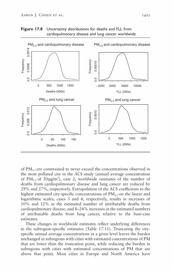
of PM2.5 are constrained to never exceed the concentrations observed inthe most polluted city in the ACS study (annual average concentrationof PM2.5 of 30mg/m3), case 2, worldwide estimates of the number ofdeaths from cardiopulmonary disease and lung cancer are reduced by29% and 27%, respectively. Extrapolation of the ACS coefficients to thehighest estimated city-specific concentrations of PM2.5 on the linear andlogarithmic scales, cases 3 and 4, respectively, results in increases of 10% and 12% in the estimated number of attributable deaths from cardiopulmonary disease, and 8–24% increases in the estimated numbersof attributable deaths from lung cancer, relative to the base-case estimates.
These changes in worldwide estimates reflect underlying differences in the subregion-specific estimates (Table 17.11). Truncating the city-specific annual average concentrations at a given level leaves the burdenunchanged in subregions with cities with estimated concentrations of PMthat are lower than the truncation point, while reducing the burden insubregions with cities with estimated concentrations of PM that areabove that point. Most cities in Europe and North America have
Aaron J. Cohen et al. 1403
Figure 17.8 Uncertainty distributions for deaths and YLL fromcardiopulmonary disease and lung cancer worldwide
Deaths (000s)
Fre
quen
cy
0 500 1000 1500
0.0
0.00
060.
0014
PM2.5 and cardiopulmonary disease PM2.5 and cardiopulmonary disease
YLL (000s)F
requ
ency
–2000 2000 6000 10000
0.0
0.00
010
Deaths (000s)
Fre
quen
cy
0 50 100 150
0.0
0.00
60.
012
PM2.5 and lung cancer PM2.5 and lung cancer
YLL (000s)
Fre
quen
cy
0 500 1000 1500
0.0
0.00
10

1404 Comparative Quantification of Health Risks
Tabl
e 17
.9(a
)A
ttri
buta
ble
deat
hs a
nd Y
LL:b
ase-
case
sce
nari
o fo
r ca
rdio
pulm
onar
y di
seas
e (5
0% a
nd 9
5% c
onfid
ence
inte
rval
s)
Subr
egio
nRe
lativ
e ris
kAt
trib
utab
le f
ract
ion
(%)
Dea
ths
(000
s)50
% C
I95
% C
IYL
L (0
00s)
50%
CI
95%
CI
AFR
-D1.
148
218
8.7–
20.4
4–31
162
80.2
–188
.336
–283
AFR
-E1.
071
19
6.1–
11.7
3–22
8459
.0–1
13.8
25–2
10
AM
R-A
1.02
92
2317
.5–2
9.0
8–38
116
87.6
–144
.741
–190
AM
R-B
1.06
63
2721
.3–3
5.5
10–4
720
115
7.4–
262.
777
–347
AM
R-D
1.10
83
42.
7–5.
01–
831
20.1
–36.
29–
60
EMR
-B1.
075
38
3.7–
8.3
1–13
6532
.0–7
0.9
11–1
11
EMR
-D1.
214
445
27.7
–51.
012
–72
386
237.
2–43
7.8
106–
618
EUR
-A1.
032
120
15.7
–26.
58–
3690
69.2
–116
.734
–156
EUR
-B1.
098
334
24.3
–41.
411
–53
238
167.
9–28
6.4
78–3
70
EUR
-C1.
046
243
26.4
–52.
412
–83
291
180.
0–35
6.9
83–5
65
SEA
R-B
1.25
04
3017
.1–3
3.8
5–50
240
136.
9–27
1.2
38–4
00
SEA
R-D
1.19
03
119
88.0
–152
.744
–198
100
674
4.7–
129
3.0
373–
167
7
WPR
-A1.
051
315
10.7
–18.
85–
2665
46.9
–81.
924
–115
WPR
-B1.
216
631
723
5.2–
402.
610
5–52
41
992
147
7.0–
252
8.5
658–
329
0
Wor
ld3
712
507.
0–87
4.7
245–
110
74
966
353
7.2–
608
3.2
169
5–7
700
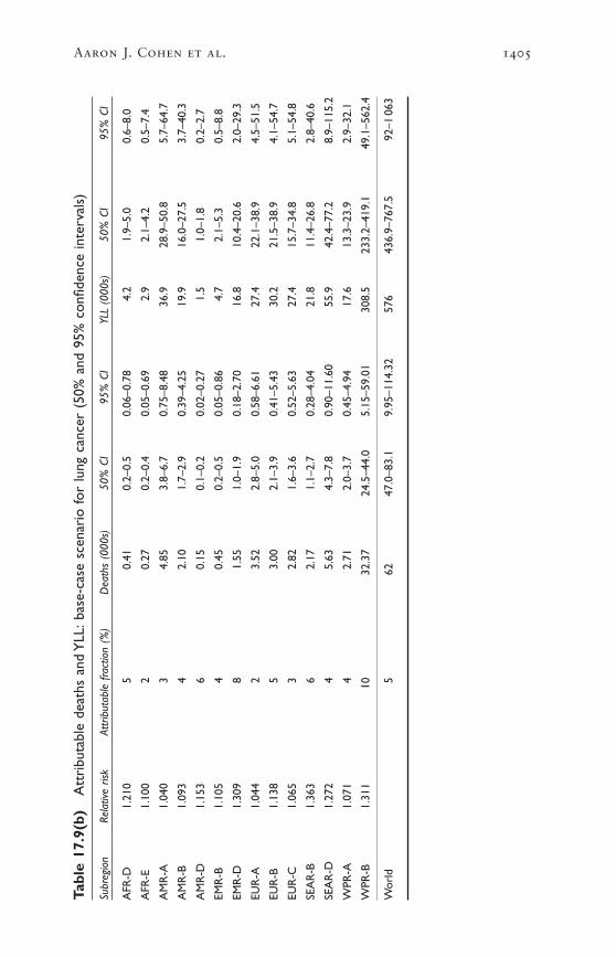
Aaron J. Cohen et al. 1405
Tabl
e 17
.9(b
)A
ttri
buta
ble
deat
hs a
nd Y
LL:b
ase-
case
sce
nari
o fo
r lu
ng c
ance
r (5
0% a
nd 9
5% c
onfid
ence
inte
rval
s)
Subr
egio
nRe
lativ
e ris
kAt
trib
utab
le f
ract
ion
(%)
Dea
ths
(000
s)50
% C
I95
% C
IYL
L (0
00s)
50%
CI
95%
CI
AFR
-D1.
210
50.
410.
2–0.
50.
06–0
.78
4.2
1.9–
5.0
0.6–
8.0
AFR
-E1.
100
20.
270.
2–0.
40.
05–0
.69
2.9
2.1–
4.2
0.5–
7.4
AM
R-A
1.04
03
4.85
3.8–
6.7
0.75
–8.4
836
.928
.9–5
0.8
5.7–
64.7
AM
R-B
1.09
34
2.10
1.7–
2.9
0.39
–4.2
519
.916
.0–2
7.5
3.7–
40.3
AM
R-D
1.15
36
0.15
0.1–
0.2
0.02
–0.2
71.
51.
0–1.
80.
2–2.
7
EMR
-B1.
105
40.
450.
2–0.
50.
05–0
.86
4.7
2.1–
5.3
0.5–
8.8
EMR
-D1.
309
81.
551.
0–1.
90.
18–2
.70
16.8
10.4
–20.
62.
0–29
.3
EUR
-A1.
044
23.
522.
8–5.
00.
58–6
.61
27.4
22.1
–38.
94.
5–51
.5
EUR
-B1.
138
53.
002.
1–3.
90.
41–5
.43
30.2
21.5
–38.
94.
1–54
.7
EUR
-C1.
065
32.
821.
6–3.
60.
52–5
.63
27.4
15.7
–34.
85.
1–54
.8
SEA
R-B
1.36
36
2.17
1.1–
2.7
0.28
–4.0
421
.811
.4–2
6.8
2.8–
40.6
SEA
R-D
1.27
24
5.63
4.3–
7.8
0.90
–11.
6055
.942
.4–7
7.2
8.9–
115.
2
WPR
-A1.
071
42.
712.
0–3.
70.
45–4
.94
17.6
13.3
–23.
92.
9–32
.1
WPR
-B1.
311
1032
.37
24.5
–44.
05.
15–5
9.01
308.
523
3.2–
419.
149
.1–5
62.4
Wor
ld5
6247
.0–8
3.1
9.95
–114
.32
576
436.
9–76
7.5
92–1
063

1406 Comparative Quantification of Health Risks
Tabl
e 17
.9(c
)A
ttri
buta
ble
deat
hs a
nd Y
LL:b
ase-
case
sce
nari
o fo
r A
RI
in c
hild
ren
aged
0–4
yea
rs (
50%
and
95%
con
fiden
cein
terv
als)
Subr
egio
nRe
lativ
e ris
kAt
trib
utab
le f
ract
ion
(%)
Dea
ths
(000
s)50
% C
I95
% C
IYL
L (0
00s)
50%
CI
95%
CI
AFR
-D1.
050
0.8
3.5
0.8–
4.9
–2.9
–9.0
119
26.8
–165
.6–9
6.0–
301.
2
AFR
-E1.
024
0.3
1.8
0.7–
3.4
–2.0
–5.8
6122
.6–1
13.5
–65.
8–19
3.3
AM
R-A
1.01
00.
00.
00.
0–0.
00.
0–0.
00
0.1–
0.3
–0.2
–0.5
AM
R-B
1.02
30.
30.
30.
1–0.
6–0
.3–0
.811
3.9–
19.1
–11.
3–27
.4
AM
R-D
1.03
70.
90.
30.
1–0.
5–0
.3–0
.911
3.2–
18.2
–10.
9–30
.3
EMR
-B1.
026
0.6
0.2
0.1–
0.3
–0.2
–0.6
71.
8–9.
6–6
.3–2
0.7
EMR
-D1.
070
1.4
4.6
1.5–
7.0
–4.1
–11.
515
551
.5–2
37.9
–137
.6–3
89.2
EUR
-A1.
011
0.0
0.0
0.0–
0.0
0.0–
0.0
00.
0–0.
1–0
.1–0
.2
EUR
-B1.
033
0.7
0.6
0.2–
1.0
–0.6
–1.5
207.
0–33
.1–2
0.1–
51.1
EUR
-C1.
016
0.1
0.1
0.0–
0.1
–0.1
–0.2
20.
6–3.
5–1
.9–5
.9
SEA
R-B
1.08
20.
50.
60.
2–1.
0–0
.6–1
.721
5.4–
35.3
–19.
7–58
.7
SEA
R-D
1.06
30.
67.
42.
6–13
.3–7
.2–2
0.1
250
86.6
–448
.4–2
43.8
–678
.5
WPR
-A1.
018
0.0
0.0
0.0–
0.0
0.0–
0.0
00.
1–0.
2–0
.1–0
.4
WPR
-B1.
071
1.2
6.1
2.0–
10.7
–6.1
–16.
520
468
.8–3
58.8
–203
.3–5
55.0
Wor
ld0.
725
.68.
2–43
.9–2
3.7–
66.1
862
277.
7–1
480.
7–7
98.6
–222
8.0
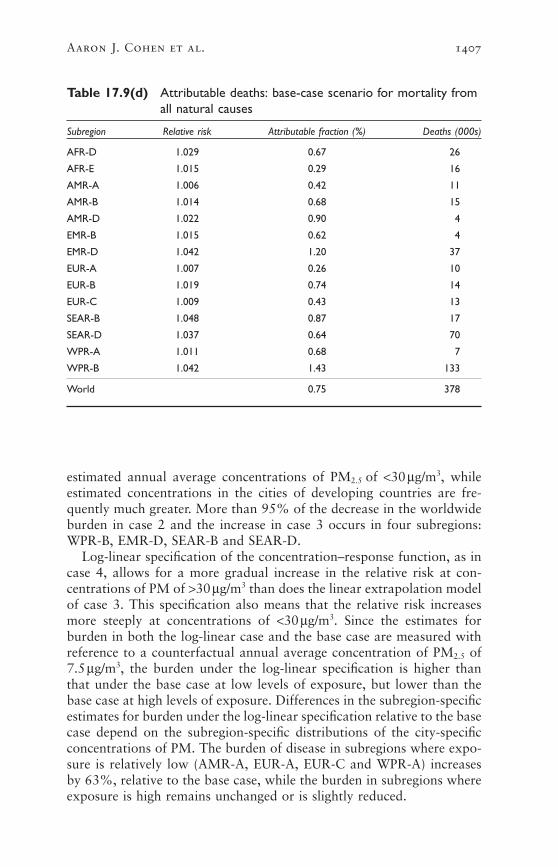
Aaron J. Cohen et al. 1407
Table 17.9(d) Attributable deaths: base-case scenario for mortality fromall natural causes
Subregion Relative risk Attributable fraction (%) Deaths (000s)
AFR-D 1.029 0.67 26
AFR-E 1.015 0.29 16
AMR-A 1.006 0.42 11
AMR-B 1.014 0.68 15
AMR-D 1.022 0.90 4
EMR-B 1.015 0.62 4
EMR-D 1.042 1.20 37
EUR-A 1.007 0.26 10
EUR-B 1.019 0.74 14
EUR-C 1.009 0.43 13
SEAR-B 1.048 0.87 17
SEAR-D 1.037 0.64 70
WPR-A 1.011 0.68 7
WPR-B 1.042 1.43 133
World 0.75 378
estimated annual average concentrations of PM2.5 of <30mg/m3, whileestimated concentrations in the cities of developing countries are fre-quently much greater. More than 95% of the decrease in the worldwideburden in case 2 and the increase in case 3 occurs in four subregions:WPR-B, EMR-D, SEAR-B and SEAR-D.
Log-linear specification of the concentration–response function, as incase 4, allows for a more gradual increase in the relative risk at con-centrations of PM of >30mg/m3 than does the linear extrapolation modelof case 3. This specification also means that the relative risk increasesmore steeply at concentrations of <30mg/m3. Since the estimates forburden in both the log-linear case and the base case are measured withreference to a counterfactual annual average concentration of PM2.5 of7.5mg/m3, the burden under the log-linear specification is higher thanthat under the base case at low levels of exposure, but lower than thebase case at high levels of exposure. Differences in the subregion-specificestimates for burden under the log-linear specification relative to the basecase depend on the subregion-specific distributions of the city-specificconcentrations of PM. The burden of disease in subregions where expo-sure is relatively low (AMR-A, EUR-A, EUR-C and WPR-A) increasesby 63%, relative to the base case, while the burden in subregions whereexposure is high remains unchanged or is slightly reduced.

1408 Comparative Quantification of Health Risks
Tabl
e 17
.10
Sens
itivi
ty a
naly
ses
of b
ase-
case
est
imat
es o
f at
trib
utab
le d
eath
s an
d Y
LL,b
y ca
use
Card
iopu
lmon
ary
dise
ase
Lung
can
cer
Acut
e re
spira
tory
infe
ctio
nsa
Attr
ibut
able
At
trib
utab
le
Attr
ibut
able
de
aths
(00
0s)
YLL
(000
s)de
aths
(00
0s)
YLL
(000
s)de
aths
(00
0s)
YLL
(000
s)Ca
seCo
nditi
ons
(% c
hang
e)(%
cha
nge)
(% c
hang
e)(%
cha
nge)
(% c
hang
e)(%
cha
nge)
Base
-cas
eM
axim
um c
once
ntra
tion
of P
M2.
5=
50mg
/m3
712
496
662
576
2686
2
Cas
e 2
Max
imum
con
cent
ratio
n of
PM
2.5=
30mg
/m3
506
(–29
)3
498
(–30
)45
(–2
7)41
4 (–
28)
NA
NA
Cas
e 3
Line
ar e
xtra
pola
tion
783
(10)
550
7 (1
1)67
(8)
623
(8)
NA
NA
Cas
e 4
Log-
linea
r ex
trap
olat
ion
794
(12)
547
6 (1
0)77
(24
)69
8 (2
1)N
AN
A
Cas
e 5
Cha
nge
AC
S co
effic
ient
/line
ar e
xtra
pola
tion
113
2 (5
9)7
908
(59)
101
(63)
939
(63)
NA
NA
Cas
e 6
Cha
nge
AC
S co
effic
ient
/log-
linea
r ex
trap
olat
ion
106
9 (5
0)7
385
(49)
105
(69)
955
(66)
NA
NA
Cas
e 7
Cha
nge
PM2.
5:P
M10
ratio
609
(–15
)4
109
(–17
)58
(–7
)52
1 (–
10)
NA
NA
Cas
e 8
The
oret
ical
min
imum
con
cent
ratio
n of
88
2 (2
4)6
081
(23)
80 (
29)
731
(27)
30 (
–15)
101
2 (–
17)
PM=
3mg
/m3
Cas
e 9
The
oret
ical
min
imum
con
cent
ratio
n of
47
4 (–
33)
336
5 (–
32)
39 (
–37)
369
(–36
)19
(27
)62
7 (2
7)PM
=15
mg/m
3
NA
Not
app
licab
le.
aIn
chi
ldre
n ag
ed–4
yea
rs.
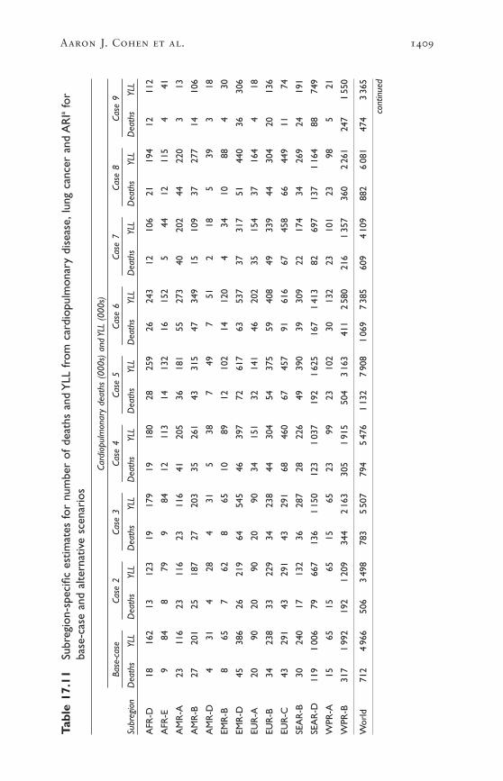
Aaron J. Cohen et al. 1409
Tabl
e 17
.11
Subr
egio
n-sp
ecifi
c es
timat
es fo
r nu
mbe
r of
dea
ths
and
YLL
fro
m c
ardi
opul
mon
ary
dise
ase,
lung
can
cer
and
AR
Iafo
rba
se-c
ase
and
alte
rnat
ive
scen
ario
s
Card
iopu
lmon
ary
deat
hs (
000s
) an
d YL
L (0
00s)
Base
-cas
eCa
se 2
Case
3Ca
se 4
Case
5Ca
se 6
Case
7Ca
se 8
Case
9
Subr
egio
nD
eath
sYL
LD
eath
sYL
LD
eath
sYL
LD
eath
sYL
LD
eath
sYL
LD
eath
sYL
LD
eath
sYL
LD
eath
sYL
LD
eath
sYL
L
AFR
-D18
162
1312
319
179
1918
028
259
2624
312
106
2119
412
112
AFR
-E9
848
799
8412
113
1413
216
152
544
1211
54
41
AM
R-A
2311
623
116
2311
641
205
3618
155
273
4020
244
220
313
AM
R-B
2720
125
187
2720
335
261
4331
547
349
1510
937
277
1410
6
AM
R-D
431
428
431
538
749
751
218
539
318
EMR
-B8
657
628
6510
8912
102
1412
04
3410
884
30
EMR
-D45
386
2621
964
545
4639
772
617
6353
737
317
5144
036
306
EUR
-A20
9020
9020
9034
151
3214
146
202
3515
437
164
418
EUR
-B34
238
3322
934
238
4430
454
375
5940
849
339
4430
420
136
EUR
-C43
291
4329
143
291
6846
067
457
9161
667
458
6644
911
74
SEA
R-B
3024
017
132
3628
728
226
4939
039
309
2217
434
269
2419
1
SEA
R-D
119
100
679
667
136
115
012
31
037
192
162
516
71
413
8269
713
71
164
8874
9
WPR
-A15
6515
6515
6523
9923
102
3013
223
101
2398
521
WPR
-B31
71
992
192
120
934
42
163
305
191
550
43
163
411
258
021
61
357
360
226
124
71
550
Wor
ld71
24
966
506
349
878
35
507
794
547
61
132
790
81
069
738
560
94
109
882
608
147
43
365
cont
inue
d

1410 Comparative Quantification of Health Risks
Tabl
e 17
.11
Subr
egio
n-sp
ecifi
c es
timat
es fo
r nu
mbe
r of
dea
ths
and
YLL
fro
m c
ardi
opul
mon
ary
dise
ase,
lung
can
cer
and
AR
Iafo
rba
se-c
ase
and
alte
rnat
ive
scen
ario
s (c
ontin
ued)
Lung
can
cer
deat
hs (
000s
) an
d YL
L (0
00s)
Base
-cas
eCa
se 2
Case
3Ca
se 4
Case
5Ca
se 6
Case
7Ca
se 8
Case
9
Subr
egio
nD
eath
sYL
LD
eath
sYL
LD
eath
sYL
LD
eath
sYL
LD
eath
sYL
LD
eath
sYL
LD
eath
sYL
LD
eath
sYL
LD
eath
sYL
L
AFR
-D0.
44.
20.
33.
20.
54.
70.
55.
01
71
70.
32.
80
50
3
AFR
-E0.
32.
90.
32.
70.
32.
90.
44.
10
51
60.
11.
50
40
1
AM
R-A
4.8
36.9
4.8
36.9
4.8
36.9
9.1
69.5
859
1294
8.4
64.4
970
14
AM
R-B
2.1
19.9
2.0
18.6
2.1
20.1
2.9
27.5
332
437
1.1
10.8
327
111
AM
R-D
0.1
1.5
0.1
1.4
0.1
1.5
0.2
2.0
02
03
0.1
0.9
02
01
EMR
-B0.
54.
70.
44.
50.
54.
70.
76.
81
71
90.
22.
41
60
2
EMR
-D1.
616
.80.
99.
52.
223
.81.
718
.43
282
251.
313
.82
191
13
EUR
-A3.
527
.43.
527
.43.
527
.46.
349
.26
449
676.
046
.96
501
6
EUR
-B3.
030
.22.
929
.03.
030
.24.
141
.05
496
564.
343
.04
392
17
EUR
-C2.
827
.42.
827
.42.
827
.44.
846
.25
446
634.
443
.14
421
7
SEA
R-B
2.2
21.8
1.2
11.9
2.6
26.2
2.2
22.0
437
331
1.6
15.7
225
217
SEA
R-D
5.6
55.9
3.7
36.8
6.4
64.0
6.2
61.6
994
986
3.9
38.5
765
441
WPR
-A2.
717
.62.
717
.62.
717
.64.
428
.34
286
384.
227
.14
261
6
WPR
-B32
.430
8.5
19.6
186.
735
.233
5.2
33.2
316.
153
503
4543
322
.020
9.6
3735
025
240
Wor
ld62
.057
645
414
6762
377
698
101
939
105
955
5852
180
731
3936
9
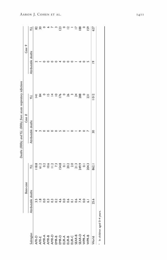
Aaron J. Cohen et al. 1411
Dea
ths
(000
s) a
nd Y
LL (
000s
) fro
m a
cute
res
pira
tory
infe
ctio
ns
Base
-cas
eCa
se 8
Case
9
Subr
egio
nAt
trib
utab
le d
eath
sYL
LAt
trib
utab
le d
eath
sYL
LAt
trib
utab
le d
eath
sYL
L
AFR
-D3.
511
8.8
414
12
82A
FR-E
1.8
61.2
384
130
AM
R-A
0.0
0.2
00
00
AM
R-B
0.3
10.6
015
06
AM
R-D
0.3
11.2
014
07
EMR
-B0.
27.
30
100
3EM
R-D
4.6
154.
85
176
412
3EU
R-A
0.0
0.1
00
00
EUR
-B0.
620
.21
260
12EU
R-C
0.1
2.0
03
01
SEA
R-B
0.6
21.3
124
117
SEA
R-D
7.4
249.
99
288
618
8W
PR-A
0.0
0.1
00
00
WPR
-B6.
120
4.3
723
15
159
Wor
ld25
.686
2.1
301
012
1962
7
aIn
chi
ldre
n ag
ed 0
–4 y
ears
.

CASES 5 AND 6: CHOICE OF ACS COEFFICIENT
Linear extrapolation beyond concentrations of PM of 30mg/m3 of largeralternative coefficients from the ACS study on the basis of the averageof ambient concentrations measured in 1979–1983 and 1999–2000resulted in increases of 59% and 63% in deaths attributable to cardiopulmonary disease and lung cancer, respectively, relative to thebase-case estimates. Log-linear extrapolation of the larger coefficientsproduced increases of 50% and 69% in the number of deaths attribut-able to cardiopulmonary disease and lung cancer, respectively (Table17.10).
Attributable burdens increased in all subregions (Table 17.11). Thedifferences between the linear and log-linear estimates followed the samesubregional patterns as in cases 3 and 4, discussed above.
CASE 7: CHOICE OF PM2.5 : PM10 RATIO
Allowing limited subregional variation in the ratio of PM2.5 to PM10 pro-duced reductions of 15% and 7% in the worldwide estimates of numbersof deaths attributable to cardiopulmonary disease and lung cancer,respectively, relative to the base-case scenario in which this ratio wasfixed at 0.50 (Table 17.10).
As one might expect, the burden of disease increases by 57% in thosesubregions assigned a ratio of 0.65, that is, AMR-A, all of Europe, andWPR-B. This increase is more than offset by the rest of the world,assigned a ratio of 0.35, where the burden of disease falls by 31% (Table17.11).
CASES 8 AND 9: CHOICE OF THEORETICAL MINIMUM LEVEL OF EXPOSURE
Halving and doubling the base-case theoretical minimum concentrationof PM2.5 of 7.5mg/m3 resulted in a 24% increase and a 33% decrease inthe number of deaths attributable to cardiopulmonary disease, and a29% increase and a 37% decrease in deaths attributable to lung cancer,but only minor variations in mortality from ARI (Table 17.10).
All subregions experienced increases in attributable burden when thetheoretical minimum concentration was halved, with the largest pro-portional increases in less polluted subregions (AMR-A, EUR-A andWPR-A). These subregions also experienced the largest reductions inburden when the theoretical minimum concentration was doubled.Highly polluted subregions (WPR-B and SEAR-D) also experiencedmarked reductions in the estimated burden when the theoreticalminimum concentration was doubled (Table 17.11).
6. DiscussionPreviously, most large-scale estimates of the health impacts of urban airpollution were conducted for countries or regions where data on expo-
1412 Comparative Quantification of Health Risks

sure and estimates of effect required for impact estimation were avail-able (e.g. Brunekreef 1997; COMEAP 1998; Künzli et al. 2000; Ostroand Chestnut 1998). In the few previous global estimates, systematicmethods were not applied to extrapolate exposures and exposure–response functions to other parts of the world (Hong 1995; WHO 1997;Working Group on Public Health and Fossil Fuel Combustion 1997).Although our estimates exceed those reported earlier, the differences arenot large, given the variation in the approaches that were taken (Smithand Mehta 2003). The global scope of the present analysis required newapproaches for estimating exposure, absent measurements of air pollu-tion in many developing countries, extrapolating the results of epidemi-ological studies more widely than had previously been attempted, anddescribing and attempting to quantify, the many uncertainties thisentailed. The results indicate that the impact of urban air pollution onthe burden of disease in the cities of the world is large and, for a varietyof reasons discussed below, have probably underestimated the burden.There is also considerable variation in our estimates among the 14 sub-regions, with the greatest burden occurring in the more polluted andrapidly growing cities of developing countries.
The availability of actual measurements of outdoor concentrations ofPM varied widely across the globe. In order to have estimates for all 14subregions, models developed by the World Bank were used to estimateconcentrations of inhalable particles (PM10) using economic, meteoro-logical and demographic data and the available measurements of PM for 3211 cities with populations of >100000, and also capital cities. Toallow the most appropriate epidemiological studies to be used for theestimation of the burden of disease, the PM10 estimates were convertedto estimates of fine particles (PM2.5) using information on geographicvariation in the ratio of PM2.5 to PM10. Population-weighted subregionalannual average exposure estimates for PM2.5 and for PM10 were obtainedusing the population of the city in the year 2000.
The estimates of the burden of disease were based on three health outcomes: mortality from cardiopulmonary causes in adults, mortalityfrom lung cancer and mortality from ARI in children aged 0–4 years.Attributable numbers of deaths and YLL for adults and children (aged0–4 years) were estimated using risk coefficients from a large cohortstudy of adults in the United States (Pope et al. 2002) and a meta-analytic summary of five time-series studies of mortality in children,respectively. Base-case estimates were calculated assuming that the riskof death increases linearly over a range of annual average concentrationsof PM2.5 between a counterfactual (or referent) concentration of 7.5 anda maximum of 50mg/m3. For comparison, an additional estimate ofattributable deaths was calculated from time-series studies of daily mor-tality, on the basis of results of a meta-analysis of the world literature,but was not used in the final calculations. Worldwide and subregion-
Aaron J. Cohen et al. 1413

specific estimates of attributable deaths and burden of disease in termsof YLL were calculated based on the standard methodology developedfor this project (see chapters 1 and 25).
We estimated that urban air pollution, as measured by PM, is respon-sible for about 3% of mortality caused by cardiopulmonary disease inadults, about 5% of mortality caused by cancers of the trachea, bronchusand lung, and about 1% of mortality caused by ARI in children world-wide in the year 2000. The total burden was about 0.80 million (1.2%of total) premature deaths and 6.4 million (0.5% of total) DALYs. Thisburden occurred predominantly in developing countries, with 30% ofattributable disease burden occurring in WPR-B and 19% in SEAR-D.The greatest contributions to the total burden of disease occurred inWPR-B, EUR-B and EUR-C, where urban air pollution caused 0.7–0.9%of the total burden of disease.
6.1 Identifying and quantifying uncertainty in the estimates
These estimates are subject to considerable uncertainty given the need toestimate exposures and to extrapolate concentration–response relation-ships. This is almost invariably the case in quantitative risk assessmentof complex environmental exposures; and is certainly to be expected inthis particular exercise, for reasons discussed above.
We quantified the statistical uncertainty of our base-case estimates byestimating the joint uncertainty in the estimates of annual average con-centration and the estimates of the relative risks. Worldwide and mostsubregional estimates vary by less than two-fold (50% uncertainty inter-vals (Tables 17.8 and 17.9[a]–[c]). Uncertainty of the model owing toassumptions about the shape of the concentration–response function, themagnitude of the relative risk of disease attributable to urban air pollu-tion, the choice of counterfactual level for PM, and the ratio of PM2.5 toPM10 was assessed in sensitivity analyses. For the most part, the estimatedworldwide burdens in the various sensitivity analyses are within the 50%uncertainty interval for the base-case estimate of worldwide burden. Thesensitivity analyses indicate that base-case estimates were most sensitiveto choice of coefficient from the ACS study and theoretical minimumconcentration.
Although some sources of uncertainty could be quantified, others thatwere no less important or were perhaps more important, could not.These additional sources of uncertainty arise from the methods we usedto estimate annual average exposure of the population and our choiceof health end-points and concentration–response functions.
ESTIMATES OF EXPOSURE TO URBAN AIR POLLUTION
There are four key uncertainties related to exposure that have not been quantified, and that could affect the estimates of burden of disease.
1414 Comparative Quantification of Health Risks
First, we used PM as the sole indicator of exposure to urban air pol-lution, although urban air pollution is a complex mixture, as notedabove. Other frequently measured pollutants, notably ozone, carbonmonoxide, oxides of sulfur and nitrogen, and lead are associated withmortality and morbidity, albeit not as consistently as PM, although theeffects of a number of these pollutants may be at least partially capturedvia the use of a PM metric (Sarnat et al. 2001). Estimating the healthimpacts of specific components poses challenges for both scientificresearch and risk assessment, including how to avoid attributing thesame burdens to multiple pollutants (i.e. double counting), and how toquantify the effects of possible interactions (i.e. synergistic effects) amongpollutants. Nonetheless, there is evidence for an effect of ozone on dailymortality that is independent of PM (e.g. Health Effects Institute 2000b).Future estimates of the burden of disease should include the healthimpacts of ozone. Unfortunately, lead in petrol remains an importanttoxic component of air pollution in some cities of the developing worldand its contribution to the burden of disease has been estimated else-where in this book (see chapter 19). Some combination of the GBD esti-mates for urban air pollution and lead probably provide the best overallestimate of the burden of disease attributable to urban air pollution.
Second, use of estimated levels of exposure introduces some uncer-tainties and biases in the predicted levels of exposure that could not beaddressed, owing to lack of data. The most important of these is the lack of city-specific data on the structure of economic activity and onfuel consumption. The exposure model uses national average data forthese variables as a reasonable proxy, which can lead to bias in unknowndirections with regard to city-specific estimates. The net bias in estimatesof the aggregate burden at the subregional level is unclear. The use oflong-run average climatic conditions instead of time-varying local datamay result in biased estimates for specific years, but may not pose aserious problem as we are interested mainly in the long-term averagehealth effects of air pollution. We have also explicitly examined ouruncertainty regarding spatial variations in the size composition of PMthrough sensitivity analysis. The model for the estimation of exposureclearly suggests that coarser particles account for a larger fraction of theTSP in developing countries than in developed countries, all other thingsbeing equal. The limited data from monitoring available on PM2.5 alsoindicate that spatial variations may also exist in the sizes of finer parti-cles. Consequently, we have used conservative estimates for the fractionof PM10 accounted for by finer particles in our overall estimates andfurther tested the implications of using an even more conservative estimate. The burden estimates should be relatively insensitive to PM sizefraction.
Third, misclassification of exposure may have led to underestimationof the burden of disease. Like the epidemiological studies used to quan-tify the estimates of health impact, we used the annual average ambient
Aaron J. Cohen et al. 1415

concentration measured from a few stationary sources in each city toestimate average personal levels of exposure. Differences between per-sonal levels of exposure and concentrations measured at fixed pointsdepend on how well the pollutant mixes in the environment and the efficiency with which the pollutant penetrates indoors. The exposure estimates are based on a model developed from population-orientedmonitors. Measurements of PM from these sites in well-designed moni-toring networks would provide representative city-wide levels of expo-sure for a pollutant that mixes uniformly in the environment. Theywould underestimate the actual level of exposure of people living nearpollution hotspots, such as busy roads or local sources of pollutant,which can contribute to spatial heterogeneity of exposure within cities(Hoek et al. 2002; Jerrett et al. 2001). This underestimate would prob-ably be more pronounced for cities in developing countries, where nearlyone third of the population resides in slums, which are often in heavily-polluted parts of cities, and even larger populations work near pollutionhotspots.
Exposure misclassification from using outdoor concentrations to rep-resent personal exposure to urban air pollution also results from differ-ences in the efficiency with which PM penetrates indoors. Use of ambientconcentrations as surrogates for exposure tends to underestimate the riskper unit exposure because the penetration of particles indoors, wheremost exposure occurs, is less than 100%. If average penetration is 66%,for example, actual exposure–response per 1mg/m3 would be 1.5-foldthat indicated by outdoor concentrations of pollution. However, becauseof climate and housing, the rates of penetration of pollution in most, butnot all, cities in developing countries can be expected to be somewhatgreater than those in the average city in the United States where the epi-demiology used here has been undertaken. Not being able to considerthis factor because of lack of data on penetration of the pollutant wouldbias estimates of burden downward if actual changes in exposures indeveloping countries are better indicated by changes in outdoor concen-trations than in developed countries.
An additional source of misclassification concerns the time referent ofour exposure estimate. The current burden is related to past exposure,but our model estimates current (i.e. 1999) levels only. However, even ifwe had been able to retrospectively estimate a time series of annualaverage concentrations for each subregion, the ACS study provides littleinformation as to how the concentration–response function varies overtime (Krewski et al. 2000). It is not clear how this source of misclassifi-cation would affect our estimates.
Fourth, our estimates do not include the attributable burden of diseaseamong the 800 million additional urban residents living either in subur-ban areas of some of the cities or in cities with populations of <100000and in the >3 billion residents of rural areas. Although lower levels ofemissions per area combined with the differences in the built-up envi-
1416 Comparative Quantification of Health Risks

ronment in rural areas probably results in a small average exposure toambient pollution and a modest increase in the global burden of diseasefrom such pollution in rural areas, the same is not true for the urbanresidents that were not included in the target population. The magnitudeof the missing burden depends on the actual exposures of those living in smaller cities. The target population was identified for the study onthe basis of data available from the United Nations, which compiles thedata reported by Member States from national censuses and makes pro-jections from them on the basis of expected changes in demographics.In compiling the population statistics, Member States, hence the UnitedNations, do not use uniform definitions either for city area (the charac-teristic such as city size that defines an urban area) or the populationincluded for each identified city (whether political boundaries are usedor agglomerations of contiguous urban areas are used). For the targetpopulation, we have used the population of the city agglomeration whenthis choice was available. If all of the remaining 800 million residentslived in suburban areas next to a targeted city, exposures and hence, esti-mates of burden, for these residents could be expected to be similar tothose in the identified city resulting in an aggregate underestimate of theattributable fraction of the population of about 28%. The exposuremodel suggests, however, that concentrations gradually decrease as thelocal population density decreases, suggesting that levels of exposure andhence estimates of burden are lower for these residents compared tothose living in larger cities. The net result is that our focus on residentsin cities with >100000 inhabitants may underestimate the aggregateburden by between 0% and 28%.
CHOICE OF HEALTH END-POINTS AND CONCENTRATION–RESPONSE FUNCTIONS
Our base-case estimates of burden in terms of disease burden consideredonly the impact of air pollution on mortality. This approach is likely tohave underestimated the true attributable burden, since there is evidencefrom studies of both epidemiology and toxicology, to suggest that airpollution may play a role in the incidence of cardiopulmonary disease,and thus contribute to years lived with disability (YLD). Lacking esti-mates of the concentration–response function for air pollution and theincidence of cardiopulmonary disease, lung cancer, and ARI in children,we calculated disease burden under the assumption that air pollutionmultiplies both incidence and mortality to the same extent, i.e. the rela-tive risk of unobserved morbidity equals the observed relative risk ofmortality (Table 17.12), an approach taken to estimating the attribut-able burden caused by other factors other than urban air pollution. The total disease burden, including YLD for cardiopulmonary disease,exceeds the YLL by 23% worldwide in the base-case analyses. The effect on the estimated burden for lung cancer and ARI in children isnegligible.
Aaron J. Cohen et al. 1417
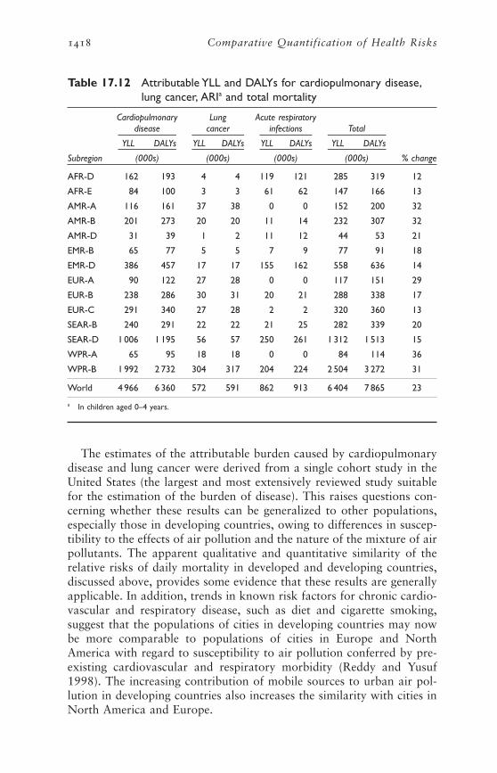
The estimates of the attributable burden caused by cardiopulmonarydisease and lung cancer were derived from a single cohort study in theUnited States (the largest and most extensively reviewed study suitablefor the estimation of the burden of disease). This raises questions con-cerning whether these results can be generalized to other populations,especially those in developing countries, owing to differences in suscep-tibility to the effects of air pollution and the nature of the mixture of airpollutants. The apparent qualitative and quantitative similarity of therelative risks of daily mortality in developed and developing countries,discussed above, provides some evidence that these results are generallyapplicable. In addition, trends in known risk factors for chronic cardio-vascular and respiratory disease, such as diet and cigarette smoking,suggest that the populations of cities in developing countries may nowbe more comparable to populations of cities in Europe and NorthAmerica with regard to susceptibility to air pollution conferred by pre-existing cardiovascular and respiratory morbidity (Reddy and Yusuf1998). The increasing contribution of mobile sources to urban air pol-lution in developing countries also increases the similarity with cities inNorth America and Europe.
1418 Comparative Quantification of Health Risks
Table 17.12 Attributable YLL and DALYs for cardiopulmonary disease,lung cancer, ARIa and total mortality
Cardiopulmonary Lung Acute respiratorydisease cancer infections Total
YLL DALYs YLL DALYs YLL DALYs YLL DALYs
Subregion (000s) (000s) (000s) (000s) % change
AFR-D 162 193 4 4 119 121 285 319 12
AFR-E 84 100 3 3 61 62 147 166 13
AMR-A 116 161 37 38 0 0 152 200 32
AMR-B 201 273 20 20 11 14 232 307 32
AMR-D 31 39 1 2 11 12 44 53 21
EMR-B 65 77 5 5 7 9 77 91 18
EMR-D 386 457 17 17 155 162 558 636 14
EUR-A 90 122 27 28 0 0 117 151 29
EUR-B 238 286 30 31 20 21 288 338 17
EUR-C 291 340 27 28 2 2 320 360 13
SEAR-B 240 291 22 22 21 25 282 339 20
SEAR-D 1 006 1 195 56 57 250 261 1 312 1 513 15
WPR-A 65 95 18 18 0 0 84 114 36
WPR-B 1 992 2 732 304 317 204 224 2 504 3 272 31
World 4 966 6 360 572 591 862 913 6 404 7 865 23
a In children aged 0–4 years.

Other sources of uncertainty in our estimates cannot be readily quan-tified for the following reasons:
• Lack of knowledge concerning differences between developed anddeveloping countries in the physicochemical nature of PM producedby different sources. The relative toxicity of PM may well vary accord-ing to the type of fuel burned and the type technology used to burnit. Increased burning of refuse outdoors and the prevalence of motorvehicles without emissions controls (e.g. vehicles powered by two-stroke engines) are two examples.
Inhalable particles that are not the direct or indirect product ofcombustion sources may also be important. These particles are mainlyof crustal origin and may be important, for example, in desert areas,or where there is disturbance of surface material owing to construc-tion, use of unsurfaced roads, etc. They are largely found in the coarsefraction of inhalable particles, whereas combustion-derived particlestend to be found in the fine and ultra-fine fractions. The evidence con-cerning the toxicity of this fraction is mixed (Anderson 2000). Dataon worldwide variation in the ratio of fine to coarse particles islimited, as discussed above, and our sensitivity analyses, which suggestrelatively minor differences with our base-case estimates, may under-state the uncertainty.
• Lack of knowledge concerning differences in the susceptibility of thepopulation. Despite the trends discussed above, differences in demog-raphy and in the patterns of the incidence and prevalence of diseasemay be associated with differences in short-term and long-term vulnerability to air pollution. There exists the possibility of effect-modification factors related to health status, and behavioural factors,such as smoking and diet (Katsouyanni et al. 2001). The effects ofprevious or concurrent exposure to high levels of indoor air pollutionmay also play a role in determining susceptibility to urban air pollu-tion. Poverty, which is a determinant of the factors just discussed, mayalso determine susceptibility in other ways. If the effects of air pollu-tion are more severe among the poor, who comprise a large part ofthe world’s population, then the magnitude of the burden would likely be greater than that which we estimated (Krewski et al. 2000; O’Neillet al. 2003).
• The shape of the exposure–response relationship may differ betweendeveloping and developed countries in ways that were not capturedin the sensitivity analyses. For example, a recent time-series study ofdaily mortality in Mexico City did not observe a flattening of the PM10 concentration–response curve until 175mg/m3 (the daily mean)(Tellez-Rojo et al. 2000). These concentrations are measured in manymega-cities in developing countries.
Aaron J. Cohen et al. 1419

We did not know which form of the concentration–response rela-tionship should be used in extrapolating the results of the ACS studyto the much higher concentrations observed in cities in India andChina, for example. For this reason, we examined the sensitivity ofthe estimates to a range of scenarios, presenting a “base case”, whichwe thought was a reasonable compromise between the conditions ofthe ACS and those of the rest of the world. Cohort evidence hasrecently been reported from Europe, although unfortunately it wasunable to estimate concentrations of PM (Hoek et al. 2002). Thisstudy provides evidence that long-term exposure to urban pollutionis associated with health effects elsewhere in developed countries, butwe still lack cohort evidence from developing countries.
MORTALITY FROM ACUTE RESPIRATORY INFECTIONS IN CHILDREN AGED
0–4 YEARS
Despite limited evidence, discussed above, linking mortality from ARI toexposure to urban air pollution, we used the results from the smallnumber of time-series studies in developing countries to estimate attrib-utable deaths and YLL in children aged 0–4 years. In our view, most ofthese deaths are likely to be among children with temporary vulnerabil-ity owing to chest infections which would resolve eventually, and there-fore represent, on average, the loss of many potential years of life, butthis view is largely speculative.
Several studies that we used to derive the concentration–responsefunction for ARI mortality actually reported results for all causes mor-tality in the 0–4 years age group (Ostro et al. 1999a), or total mortalityin the first year of life (Loomis et al. 1999). We have assumed that therelationship between PM10 and mortality from ARI in children aged 0–4 years is similar to that for all-cause mortality. To some extent thisis justified by the knowledge that mortality from ARI is an important component of all-cause mortality in developing countries.
6.2 Generalizability of our results
As a consequence of the uncertainties in this global assessment, its quan-titative results cannot be confidently extrapolated to smaller geographicareas, such as specific countries or cities. The methods for estimation ofexposure and extrapolation of concentration–response functions weredeveloped specifically for estimating burdens for large geographicregions, often in the absence of essential data on exposure and response.Where better data exist, as they currently do in some parts of the world,they can, of course, be used.
Differences between our estimates and those of other groups mayreflect other differences in methodology. For example, a tri-national Euro-pean assessment recently estimated that some 40000 deaths per year wereattributable to exposure to ambient air pollution in a population ofapproximately 72 million, whereas the burden in EUR-A, in an urban
1420 Comparative Quantification of Health Risks

population of 80 million, was estimated to be 23000 deaths per year, de-spite similar estimates of the concentration of ambient pollution (Künzliet al. 2000). The difference is largely owing to the different assumptionsregarding the exposure reference level of 15mg/m3 PM10 in this work vs7.5mg/m3 in the European study. In addition, the concentration–responsefunctions were slightly higher in the tri-national project, which used esti-mates of total mortality from both the first ACS publication and theHarvard Six City estimates (Dockery et al. 1993; Pope et al. 1995).
6.3 Avoidable disease burden
We did not attempt to estimate the avoidable burden of disease, despitethis being a specific objective of the project. Estimating the avoidableburden would have required making projections of concentrations ofambient air pollution and providing a model for the exposuretime–response function for PM and mortality. Time constraints did notallow us to undertake the former task, although it is feasible. The latterinformation is not currently available from the existing cohort studies,although there is limited evidence that the induction time for mortalityfrom lung cancer attributable to exposure to urban air pollution is in theorder of decades (Nyberg et al. 2000), and that it is perhaps in the orderof years for mortality from cardiovascular disease (Krewski et al. 2000).Evaluations of both “natural experiments” (Heinrich et al. 2000; Pope1989), and regulatory interventions (Clancy et al. 2002; Hedley et al.2002) provide further support for relatively rapid improvements in car-diovascular and respiratory outcomes. The latter studies also suggest thatalthough rates of mortality may decrease after the successful imple-mentation of air pollution reductions, the long-term benefits may extendwell beyond that observed during the first years after the intervention isimplemented.
6.4 How could a future risk assessment exercise provide better estimates?
There is a critical need for more information on the health effects of airpollution in developing counties. Research on exposure should aim toprovide better estimates not only of ambient concentrations of pollu-tants, but also the characteristics of urban air pollution, including thecontribution of various sources and the size distribution of PM. Epidemiological studies of mortality should be designed to provide age-and disease-specific estimates of the effects of air pollution, as well asidentifying factors that confer susceptibility to air pollution. There is anobvious need for epidemiological studies of the effect of air pollution onthe incidence of chronic cardiovascular and respiratory disease, and onthe growth and development of children. Future estimates of the burdenof disease attributable to urban air pollution should include morbidityoutcomes, such as asthma exacerbation, which most certainly contributeto morbidity.
Aaron J. Cohen et al. 1421

Estimates of uncertainty distributions should more fully incorporatemodel uncertainties, such as those related to the choice of concentra-tion–response function. This could be accomplished via the elicitationand weighting of expert opinions in the context of a Bayesian approachto quantifying model uncertainty (Morgan and Henrion 1998; NationalResearch Council 2002).
AcknowledgementsThe authors wish to acknowledge the contribution of Richard Burnett,Uwe Deichmann, Majid Ezzati, Stephen Vander Hoorn and DavidWheeler.
DisclaimerThe views expressed in this paper are those of the authors and do notnecessarily reflect the views of the Health Effects Institute (HEI) or itssponsors nor those of the World Bank.
Notes1 Throughout the chapter we refer to urban air pollution using the terms
“ambient air pollution” or “urban air pollution”. For our current purposes,these terms are fully interchangeable.
2 See Preface for an explanation of this term.
3 Ambient particles fall into a trimodal size distribution, according to theiraerodynamic diameter: coarse particles (>1 mm), fine particles (0.1–1 mm), andultrafine particles (<0.1 mm). Ultrafine particles constitute a small percentageof the total mass of PM, but are present in very high numbers. Because ofhealth concerns, the ambient concentrations (mass) of both coarse and finePM are regulated by the United States Environmental Protection Agency(EPA) through the National Ambient Air Quality Standards for PM10 (PM <10 mm) and PM2.5 (PM <2.5 mm) (USEPA 1997), and by the European Unionthrough limit values for PM10. PM2.5, which includes only fine and ultrafineparticles, is dominated by emissions from combustion processes; PM10, whichincludes coarse as well as fine and ultrafine particles, has a much higher pro-portion of particles generated by mechanical processes from a variety of non-combustion sources. It is currently not clear how much particles of differentsizes and composition differ in the effects on health that they cause.
4 Cities in the United States account for about 40% of the observations in theestimation model, even after this exclusion.
5 Data from monitoring were available for one additional city/country, Skopjein The former Yugoslav Republic of Macedonia, but were not used in theestimation model because of missing explanatory variables. In addition, 150observations primarily from Germany (94), Lithuania (30) and other easternEuropean states (26) made during the early 1990s were excluded because ofuncertainties in defining appropriate explanatory variables.
1422 Comparative Quantification of Health Risks

6 The model presented here is one of several versions of the GMAPS modeldeveloped at the World Bank. An alternative model jointly estimates con-centrations of PM10 and TSP at residential and non-residential sites.
7 The climatic variables have been constructed from a global mean monthlyclimatology map with a resolution of 0.5° latitude ¥ 0.5° longitude developed by researchers at the Climate Research Unit of the University ofEast Anglia. These data are available at http://ipcc-ddc.cru.uea.ac.uk/cru_data/examine/have_index.html. All of the climate variables are based on theconditions for the city centre.
8 Residential monitoring sites are located in residential areas but do not includepollution hotspots, such as locations that are immediately adjacent to indus-trial and commercial pollution sources or high traffic corridors. In contrast,mixed residential sites are characterized by both high population densitiesand the presence of some pollution sources that may result in elevated con-centrations of PM in the immediate vicinity of the pollution source. Neithersite includes areas of high pollution activity located in sparsely populatedareas.
9 Had we instead included data from monitoring for cities with measured data for 1999, there would be an insignificant difference in the subregionalaverage concentration, because a small fraction of the population in eachsubregion lives in monitored cities and most of the monitored cities arelocated in North America and western Europe, where the estimates of PMare more precise.
10 After these estimates had been made, investigators in the United States andCanada discovered several problems with the statistical software that hadbeen used to estimate the relative risks associated with air pollution in thetime-series studies (Health Effects Institute 2003). Correcting these problemsreduced the magnitude of estimated relative risks and increased their stan-dard errors.
ReferencesAbbey DE, Nishino N, McDonnell WF et al. (1999) Long-term inhalable parti-
cles and other air pollutants related to mortality in nonsmokers. AmericanJournal of Respiratory and Critical Care Medicine, 159:373–382.
Aerometric Information Retrieval System (2001) U.S. Environmental ProtectionAgency, Office of Air Quality Planning and Standards, AIRS. Available athttp://www.epa.gov/oar/oaqps/airpdata.html#airs.
American Thoracic Society (ATS) (2000) What constitutes an adverse healtheffect of air pollution? American Journal of Respiratory and Critical CareMedicine, 161:665–673.
Anonymous (1996a) Health effects of outdoor air pollution. Part 1. Committeeof the Environmental and Occupational Health Assembly of the AmericanThoracic Society. American Journal of Respiratory and Critical Care Medi-cine, 153:3–50.
Anonymous (1996b) Health effects of outdoor air pollution. Part 2. Committeeof the Environmental and Occupational Health Assembly of the American
Aaron J. Cohen et al. 1423
Thoracic Society. American Journal of Respiratory and Critical Care Medicine, 153:477–498.
Anonymous (1998) Worldwide variations in the prevalence of asthma symptoms:the International Study of Asthma and Allergies in Childhood (ISAAC). European Respiratory Journal. 12:315–335.
Anderson HR (2000) Differential epidemiology of ambient aerosols. Philo-sophical Transactions of the Royal Society of London, Series A, 358:2771–2785.
Atkinson RW, Anderson HR, Sunyer J et al. (2001) Acute effects of particulateair pollution on respiratory admissions: results from APHEA 2 project. Airpollution and health: a European approach. American Journal of Respiratoryand Critical Care Medicine, 164:1860–1866.
Awasthi S, Glick HA, Fletcher RH, Ahmed N (1996) Ambient air pollution andrespiratory symptoms complex in preschool children. Indian Journal ofMedical Research, 104:257–262.
Bacharova L, Fandakova K, Bratinka J, Budinska M, Bachar J, Gud-aba M(1996) The association between air pollution and the daily number ofdeaths: findings from the Slovak Republic contribution to the APHEAproject. Journal of Epidemiology and Community Health, 50:S19–21.
Begg CB, Mazumdar M (1994) Operating characteristics of a rank correlationtest for publication bias. Biometrics, 50:1088–1101.
Bobak M, Leon DA (1999) The effect of air pollution on infant mortality appearsspecific for respiratory causes in the post neonatal period. Epidemiology,10:666–670.
Borja-Aburto VH, Castillejos M, Gold DR, Bierzwinski S, Loomis D (1998)Mortality and ambient fine particles in southwest Mexico City, 1993–1995.Environmental Health Perspectives, 106:849–855.
Borja-Aburto VH, Loomis DP, Bangidiwala SI, Shy CM, Rascon-Pacheco RA(1997) Ozone, suspended particulates, and daily mortality in Mexico City.American Journal of Epidemiology, 145:258–268.
Braga AL, Zanobetti A, Schwartz J (2001) The lag structure between particulateair pollution and respiratory and cardiovascular deaths in 10 US cities.Journal of Occupational and Environmental Medicine, 43:927–933.
Brunekreef B (1997) Air pollution and life expectancy: is there a relation? Occu-pational and Environmental Medicine, 54:781–784.
Burnett RT, Smith-Doiron M, Stieb D, Cakmak S, Brook JR (1999) Effects ofparticulate and gaseous air pollution on cardiorespiratory hospitalizations.Archives of Environmental Health, 54:130–139.
Burney PG, Luczynska C, Chinn S, Jarvis D (1994) The European CommunityRespiratory Health Survey. European Respiratory Journal, 7:954–960.
California Air Resources Board (2002) Staff report: Public hearing to consideramendments to the ambient air quality standards for particulate matter andsulfates. California Air Resources Board and Office of Environmental HealthHazard Assessment, Sacramento, CA.
1424 Comparative Quantification of Health Risks

Calle EE, Rodriguez C, Jacobs EJ et al. (2002) The American Cancer SocietyCancer Prevention Study II Nutrition Cohort: rationale, study design, andbaseline characteristics. Cancer, 94:2490–2501.
Castillejos M, BorjaAburto VH, Dockery DW, Gold DR, Loomis D (2000) Airborne coarse particles and mortality. Inhalation Toxicology, 12:61–72.
CIESIN (2000) Gridded population of the world (GPW), version 2. Center forInternational Earth Science Information Network (CIESIN), Columbia University; International Food Policy Research Institute (IFPRI), WorldResources Institute (WRI) Columbia University, Palisades, NY. Available athttp://sedac.ciesin.columbia.edu/plue/gpw.
Chay KY, Greenstone M (1999) The impact of air pollution on infant mortal-ity: evidence from geographic variation in pollution shocks induced by a reces-sion. Unpublished document. (Working Paper No. 17.) Available from: Centerfor Labor Economics, University of California, Berkeley, CA.
Chay KY, Greenstone M (2001) Air quality, infant mortality, and the Clean Air Act of 1970. Unpublished document. (Working Paper No. 42.) Availablefrom: Center for Labor Economics, University of California, Berkeley, CA.
Chhabra SK, Chhabra P, Rajpal S, Gupta RK (2001) Ambient air pollution andchronic respiratory morbidity in Delhi. Archives of Environmental Health,56:58–64.
Cifuentes L, Borja-Aburto VH, Gouveia N, Thurston G, Davis DL (2001) Assessing the health benefits of urban air pollution reductions associated with climate change mitigation (2000–2020): Santiago, São Paulo, MexicoCity, and New York City. Environmental Health Perspectives, 109:S419–425.
Cifuentes L, Vega J, Kopfer K, Lava LB (2000) Effect of the fine fraction of par-ticulate matter versus the coarse mass and other pollutants on daily mor-tality in Santiago, Chile. Journal of the Air Waste Management Association,50:1287–1298.
Clancy L, Goodman P, Sinclair H, Dockery DW (2002) Effect of air pollutioncontrol on death rates in Dublin, Ireland: an intervention study. The Lancet,360:1210–1214.
Cohen AJ, Nikula K (1999) Health effects of diesel exhaust: laboratory and epidemiologic studies. In: Air pollution and health. Holgate ST, Samet JM,Koren HS, Maynard R, eds. Academic Press, London.
COMEAP (1998) Quantification of the effects of air pollution on health in theUnited Kingdom. Department of Health Committee on the Medical Effectsof Air Pollutants. Stationery Office, London.
COMEAP (2001) Statement on long term effects of particles on mortality. Avail-able at http://www.doh.gov.uk/comeap/state.htm, or as a printable documentat http://www.doh.gov.uk/comeap/statementsreports/longtermeffects.pdf.
Conceiao GMS, Miraglia SGEK, Kishi HS, Saldiva PNH, Singer JM (2001) Air pollution and child mortality: a time series study in São Paulo, Brazil.Environmental Health Perspectives, 109:347–350.
Aaron J. Cohen et al. 1425

Daniels MJ, Dominici F, Samet JM, Zeger SL (2000) Estimating particulatematter-mortality dose-response curves and threshold levels: an analysis ofdaily time-series for the 20 largest US cities. American Journal of Epidemiol-ogy, 152:397–406.
Derwent RG (1999) Atmospheric chemistry. In: Air pollution and health.Holgate ST, Samet JM, Koren HS, Maynard R, eds. Academic Press, London.
Diesel Working Group (1995) Diesel exhaust: a critical analysis of emissions,exposure, and health effects. Special report. Health Effects Institute, Cambridge, MA.
Dockery DW, Pope AC, Xu X et al. (1993) An association between air pollutionand mortality in six US cities. New England Journal of Medicine, 329:1753–1759.
Ezzati M, Lopez AD, Rodgers A, Vander Hoorn S, Murray CJL, Comparative Risk Assessment Collaborating Group (2002). Selected majorrisk factors and global and regional burden of disease. The Lancet, 360:1347–1360.
Gao J (1993) [Relationship between air pollution and mortality in Dongchengand Xicheng Districts, Beijing]. Chung-Hua Yu Fang i Hsueh Tsa Chih[Chinese Journal of Preventive Medicine], 27:340–343.
Gouveia N, Fletcher T (2000) Time series analysis of air pollution and mortal-ity: effects by cause, age and socioeconomic status. Journal of Epidemiologyand Community Health, 54:750–755.
Grant LD, Shoaf CR, Davis JM (1999) Sources of air pollution. In: Air pollu-tion and health. Holgate ST, Samet JM, Koren HS, Maynard R, eds. Acade-mic Press, London.
Grønskei KE, Gram F, Hagen LO et al. (1997a) URBAIR Urban air quality man-agement strategy in Asia: Jakarta report. Shah J, Nagpal T, eds. World Bank,Washington, DC.
Grønskei KE, Gram F, Hagen LO et al. (1997b) URBAIR Urban air quality man-agement strategy in Asia: Kathmandu Valley report. Shah J, Nagpal T, eds.World Bank, Washington, DC.
Hajat S, Anderson HR, Atkinson RW, Haines A (2002) Effects of air pollutionon general practitioner consultations for upper respiratory diseases inLondon. Occupational and Environmental Medicine, 59:294–299.
Hajat S, Haines A, Atkinson RW, Bremner SA, Anderson HR, Emberlin J (2001)Association between air pollution and daily consultations with general prac-titioners for allergic rhinitis in London, United Kingdom. American Journalof Epidemiology, 153:704–714.
Hales S, Salmond C, Town GI, Kjellstrom T, Woodward A (2000) Daily mor-tality in relation to weather and air pollution in Christchurch, New Zealand. Australia and New Zealand Journal of Public Health, 24:89–91.
Health Effects Institute (2000a) National morbidity, mortality and air pollutionstudy. (HEI Report No. 94, Part 1. Methods and methodologic issues) HealthEffects Institute. Cambridge, MA.
1426 Comparative Quantification of Health Risks
Health Effects Institute (2000b) National morbidity, mortality and air pollutionstudy. (HEI Report No. 94. Part 2.) Health Effects Institute. Cambridge, MA.
Health Effects Institute (2001) Airborne particles and health: HEI epidemiologicevidence. HEI perspectives. Health Effects Institute, Cambridge, MA.
Health Effects Institute (2002) Understanding the health effects of componentsof the particulate matter mix: progress and next steps. HEI Perspectives.Health Effects Institute, Boston, MA.
Health Effects Institute (2003) Revised analyses of time-series studies of air pol-lution and health. Health Effects Institute. Boston, MA.
Hedley AJ, Wong CM, Thach TQ, Ma S, Lam TH, Anderson HR (2002)Cardiorespiratory and all-cause mortality after restrictions on sulphur content of fuel in Hong Kong: an intervention study. The Lancet, 360:1646–1652.
Heinrich J, Hoelscher B, Wichmann HE (2000) Decline of ambient air pollutionand respiratory symptoms in children. American Journal of Respiratory andCritical Care Medicine, 161:1930–1936.
Hoek G, Brunekreef B, Goldbohm S, Fischer P, van den Brandt PA (2002) Asso-ciation between mortality and indicators of traffic-related air pollution in theNetherlands: a cohort study. The Lancet, 360:1203–1209.
Holman C (1999) Sources of air pollution. In: Air pollution and health. HolgateST, Samet JM, Koren HS, Maynard R, eds. Academic Press, London.
Hong C (1995) Global burden of disease from air pollution. World Health Orga-nization, Geneva. Available athttp://www.cru.uea.ac.uk/~markn/cru05/cru05_intro.html.
Hong YC, Leem JH, Ha EH (1999) Air pollution and daily mortality in Inchon,Korea. Journal of Korean Medical Science, 14:239–244.
Hong YC, Leem JH, Ha EH, Christiani DC (1999) PM10 exposure, gaseous pol-lutants, and daily mortality in Inchon, South Korea. Environmental HealthPerspectives, 107:873–888.
Hurley F, Holland MR, Markandya A et al. (2000) Towards assessing andcosting the health impacts of ambient particulate air pollution in the UK.(Report TM/00/07.) Institute of Occupational Medicine, Edinburgh.
Instituto Nacional de Ecología (2000) Almanaque de datos y tendencias de lacalidad del aire en ciudades Mexicanas [Temperature data and trends inMexican cities], Dirección General de Gestión e Información Ambiental delInstituto Nacional de Ecología, Secretaría de Medio Ambiente y RecursosNaturales (SEMARNAP) [The Secretariat of Environment and NaturalResources], Mexico. Unpublished document, available at http://www.ine.gob.mx.
International Energy Agency (2001a) Energy balance of non-OECD countries1995–1999. International Energy Agency, Vienna.
International Energy Agency (2001b) Energy Balance of OECD Countries1995–1999. International Energy Agency, Vienna.
Aaron J. Cohen et al. 1427

Jerrett M, Burnett RT, Kanaroglou P et al. (2001) A GIS-environmental justiceanalysis of particulate air pollution in Hamilton, Canada. Environment andPlanning A, 33:955–973.
Katsouyanni K, Schwartz J, Spix C et al. (1996) Short term effects of air pollution on health: a European approach using epidemiologic time seriesdata: the APHEA protocol. Journal of Epidemiology and Community Health,50:S12–18.
Katsouyanni K, Touloumi G, Samoli E et al. (2001) Confounding and effect mod-ification in the short-term effects of ambient particles on total mortality:results from 29 European cities within the APHEA2 project. Epidemiology,12:521–531.
Krewski D, Burnett RT, Goldberg MS et al. (2000) Reanalysis of the HarvardSix Cities Study and the American Cancer Society Study of particulate air pol-lution and mortality. A special report of the institute’s particle epidemiologyreanalysis project. Health Effects Institute, Cambridge, MA.
Krzyzanowski M, Schwela D (1999) Patterns of air pollution in developing coun-tries. In: Air pollution and health. Holgate ST, Samet JM, Koren HS, MaynardR, eds. Academic Press, London.
Krzyzanowski M, Wojtyniak B (1991) Air pollution and daily mortality inCracow. Public Health Reviews, 19:73–81.
Künzli N, Kaiser R, Medina S et al. (2000) Public-health impact of outdoor and traffic-related air pollution: a European assessment. The Lancet, 356:795–801.
Künzli N, Medina S, Kaiser R et al. (2001) Assessment of deaths attributable toair pollution: should we use risk estimates based on time series or cohortstudies? American Journal of Epidemiology, 153:1050–1055.
Lee J-T, Kim H, Hong YC, Kwon HJ, Schwartz J, Christiani DC (2000) Air pollution and daily mortality in seven major cities of Korea, 1991–1997.Environmental Research, 84:247–254.
Lee J-T, Shin D, Chung Y (1999) Air pollution and daily mortality in Seoul andUlsan, Korea. Environmental Health Perspectives, 107:149–154.
Leksell I, Rabl A (2001) Air pollution and mortality: quantification and valua-tion of years of life lost. Risk Analysis, 21:843–857.
Levy JI, Hammitt JK, Spengler JD (2000) Estimating the mortality impacts ofparticulate matter: what can be learned from between-study variability? Envi-ronmental Health Perspectives, 108:109–117.
Lipfert FW, Perry HM Jr, Miller JP, Baty JD, Wyzga RE, Carmody SE (2003) Airpollution, blood pressure, and their long-term associations with mortality.Inhalation Toxicology, 15:493–512.
Loomis D, Castillejos M, Gold DR et al. (1999) Air pollution and infant mor-tality in Mexico City. Epidemiology, 10:118–123.
McDonnell WF, Nishino-Ishikawa N, Petersen FF, Chen LH, Abbey DE (2000)Relationships of mortality with the fine and coarse fractions of long-termambient PM10 concentrations in nonsmokers. Journal of Exposure Analysisand Environmental Epidemiology, 10:427–436.
1428 Comparative Quantification of Health Risks

McMichael AJ, Anderson HR, Brunekreef B, Cohen AJ (1998) Inappropriate useof daily mortality analyses to estimate longer-term mortality effects of air pol-lution. International Journal of Epidemiology, 27:450–453.
Morgan MG, Henrion M (1998) Uncertainty: a guide to dealing with uncer-tainty in quantitative risk and policy analysis. Cambridge University Press,Cambridge.
National EPA of China (2000) Environmental statistical yearbook. China Envi-ronmental Publishing House, Beijing.
National Research Council (2002) Estimating the public health benefits of proposed air pollution regulations. National Academies Press, Washington,DC.
Navidi W, Lurmann F (1995) Measurement error in air pollution exposureassessment. Journal of Exposure Analysis and Environmental Epidemiology,5:111–124.
New M, Hulme M, Jones P (1999) Representing twentieth-century space-timeclimate variability. Part I. Development of a 1961–90 mean monthly terres-trial climatology, Journal of Climate, 12:829–856.
Nyberg F, Gustavsson P, Jarup L et al. (2000) Urban air pollution and lung cancerin Stockholm. Epidemiology, 11:487–495.
O’Neill M, Jerrett M, Kawachi I et al. (2003) Health, wealth and air pollution.Environmental Health Perspectives, 111:1861–1870.
Ostro B, Chestnut L (1998) Assessing the health benefits of reducing particulatematter air pollution in the United States. Environmental Research, 76:94–106.
Ostro B, Chestnut L, Vichit-Vadakan N, Laixuthai A (1999a). The impact ofparticulate matter on daily mortality in Bangkok, Thailand. Journal of theAir and Waste Management Association 49:100–107.
Ostro B, Hurley S, Lipsett MJ (1999b) Air pollution and daily mortality in theCoachella Valley, California: a study of PM10 in an area dominated by coarseparticles. Environmental Research, 81:231–238.
Ostro BD, Sanchez JM, Aranda C, Eskeland GS (1996) Air pollution and mortality: results from a study of Santiago, Chile. Journal of ExposureAnalysis and Environmental Epidemiology, 6:97–114.
Ozkaynak H (1999) Exposure assessment. In: Air pollution and health. HolgateST, Samet JM, Koren HS, Maynard R, eds. Academic Press, London.
Pandey KD, Wheeler D, Ostro B, Deichmann U, Hamilton K, Bolt K (forth-coming) Ambient particulate matter concentrations in residential areas ofworld cities: new estimates based on global model of ambient particulates(GMAPS). The Development Research Group and the Environment Depart-ment, World Bank, Washington, DC.
Pereira LA, Loomis D, Conceicao GM et al. (1998) Association between air pol-lution and intrauterine mortality in São Paulo, Brazil. Environmental HealthPerspectives, 106:325–329.
Peters A, Dockery DW, Muller JE, Mittleman MA (2001) Increased particulateair pollution and the triggering of myocardial infarction. Circulation, 103:2810–2815.
Aaron J. Cohen et al. 1429
Pope CA III (1989) Respiratory disease associated with community air pollutionand a steel mill, Utah Valley. American Journal of Public Health, 79:623–628.
Pope CA III, Burnett RT, Thun MJ et al. (2002) Lung cancer, cardiopulmonarymortality, and long-term exposure to fine particulate air pollution. Journal ofthe American Medical Association, 287:1132–1141.
Pope CA III, Dockery DW (1999) Epidemiology of particle effects. In: Air pollution and health. Holgate ST, Samet JM, Koren HS, Maynard R, eds. Academic Press, London.
Pope CA III, Thun MJ, Namboodiri MM et al. (1995) Particulate air pollutionas a predictor of mortality in a prospective study of US adults. AmericanJournal of Respiratory and Critical Care Medicine, 151:669–674.
Qian Z, Chapman RS, Tian Q, Chen Y, Lioy PJ, Zhang J (2000) Effects of airpollution on children’s respiratory health in three Chinese cities. Archives ofEnvironmental Health, 55:126–133.
Qian Z, Zhang J, Wei F, Wilson WE, Chapman RS (2001) Long term ambientair pollution levels in four Chinese cities: inter-city and intra-city concentra-tion gradients for epidemiological studies. Journal of Exposure Analysis andEnvironmental Epidemiology, 11:341–351.
Reddy KS, Yusuf S (1998) Emerging epidemic of cardiovascular disease in devel-oping countries. Circulation, 97:596–601.
Roemer W, Clench-Aas J, Englert N et al. (1999) Inhomogeneity in response toair pollution in European children (PEACE project). Occupational and Envi-ronmental Medicine, 56:86–92.
Romieu I, Samet JM, Smith KR, Bruce N (2002) Outdoor air pollution and acuterespiratory infections among children in developing countries. Journal ofOccupational and Environmental Medicine, 44:640–649.
Saldiva PHN, Lichtenfels AJFC, Paiva PSO et al. (1994) Association between airpollution and mortality due to respiratory diseases in children in São Paulo,Brazil: a preliminary report. Environmental Research, 65:218–225.
Saldiva PH, Pope CA, III, Schwartz J et al. (1995) Air pollution and mortalityin elderly people: a time-series study in São Paulo, Brazil. Archives of Envi-ronmental Health, 50:159–163.
Samet JM (1999) Air pollution and risk assessment. In: Air pollution and health.Holgate ST, Samet JM, Koren HS, Maynard R, eds. Academic Press, London.
Samet JM, Cohen AJ (1999) Air pollution and lung cancer. In: Air pollution andhealth. Holgate ST, Samet JM, Koren HS, Maynard R, eds. Academic Press,London.
Sanhueza P, Vargas C, Jimenez J (1999) Daily mortality in Santiago and its rela-tionship with air pollution. Revista Medica de Chile, 127:235–242.
Sarnat JA, Schwartz J, Catalano PJ, Suh HH (2001) Gaseous pollutants in par-ticulate matter epidemiology: confounders or surrogates? EnvironmentalHealth Perspectives, 109:1053–1061.
Schwartz J (2000) Harvesting and long-term exposure effects in the relationbetween air pollution and mortality. American Journal of Epidemiology,151:440–448.
1430 Comparative Quantification of Health Risks

Schwartz J, Laden F, Zanobetti A (2002) The concentration-response relationbetween PM(2.5) and daily deaths. Environmental Health Perspectives,110:1025–1029.
Simpson R, Denison L, Petroeschevsky A, Thalib L, Williams G (2000) Effectsof ambient particle pollution on daily mortality in Melbourne, 1991–1996.Journal of Exposure Analysis and Environmental Epidemiology, 10:488–496.
Smith KR, Mehta S (2003) The burden of disease from indoor air pollution indeveloping countries: comparison of estimates. International Journal ofHygiene and Environmental Health, 206:279–89.
Sommer H, Künzli N, Seethaler R et al. (2000) An impact assessment project ofAustria, France and Switzerland. Ancillary benefits and costs of greenhousegas mitigation (Proceedings from an OECD Expert Workshop). OECD, NewYork.
Stanfield JP (1993) Some aspects of the long-term effects of malnutrition on thebehaviour of children in the Third World. Proceedings of the NutritionalSociety, 52:201–210.
Stieb DM, Judek S, Burnett RT (2003) Meta-analysis of time-series studies of airpollution and mortality: update in relation to the use of generalized additivemodels. Journal of the Air and Waste Management Association, 53:258–261.
Szafraniec K, Tecza W (1999) The effect of short-term changes in levels of airpollution on mortality from cardiovascular diseases among inhabitants ofKrakow [in Polish]. Przeglad Lekarski, 56:698–703.
Tager IB, Künzli N, Lurmann F, Ngo L, Segal M, Balmes J (1998) Methods devel-opment for epidemiologic investigations of the health effects of prolongedozone exposure. Part II. An approach to retrospective estimation of lifetimeozone exposure using a questionnaire and ambient monitoring data (Califor-nia sites). (Research Report No. 81.) Health Effects Institute, Cambridge,MA.
Tellez-Rojo MM, Romieu I, Ruiz-Velasco S, Lezana MA, Hernandez-Avila MM(2000) Daily respiratory mortality and PM10 pollution in Mexico City:importance of considering place of death. European Respiratory Journal,16:391–396.
UN (2001) Demographic yearbook 1998. (United Nations Publication, Sales No.E/F.97.XIII.1.) Data also available at http://unstats.un.org/unsd/citydata/.
U.S. Environmental Protection Agency (1996) Review of the national ambientair quality standards for particulate matter: policy assessment of scientific andtechnical information: OAQPS staff paper (EPA-452\R-96-013.) Office of AirQuality Planning and Standards, Research Triangle Park, NC.
U.S. Environmental Protection Agency (1997) National ambient air quality stan-dards for particulate matter: final rule. (CFR Part 50, Federal register62:1–54.) U.S. Environmental Protection Agency, Washington, DC.
U.S. Environmental Protection Agency (2002) Third external review draft of airquality criteria for particulate matter, April 2002. (EPA/600/p-99/002aC.)Office of Research and Development, Washington, DC.
Aaron J. Cohen et al. 1431

USGS (1996) GTOPO30—Global digital elevation model, US geological survey.Eros Data Center, Sioux Falls, SD. Available at http://edcdaac.usgs.gov/gtopo30/gtopo30.asp.
WHO (1997) Health and environment in sustainable development: five yearsafter the earth summit. World Health Organization, Geneva.
WHO (2000a) Air quality guidelines for Europe. Second edition. (WHORegional Publication, European Series, No. 91.) WHO Regional Office forEurope, Copenhagen.
WHO (2000b) Evaluation and use of epidemiological evidence for environmen-tal health risk assessment. (EUR/00/5020369.) WHO Regional Office forEurope, Copenhagen.
WHO (2001a) Health impact assessment of air pollution in the WHO EuropeanRegion. (Technical Report from WHO/ECEH Project.) WHO EuropeanCentre for Environment and Health, Bonn.
WHO (2001b) Quantification of health effects of exposure to air pollution.WHO Regional Office for Europe. Available at http://www.euro.who.int/document/e74256.pdf.
WHO (2001c) Air quality and health. Air Management Information SystemAMIS3.0. World Health Organization, Geneva.
WHO (2002) World health report 2002. Reducing risks, promoting healthy life.World Health Organization, Geneva.
WHO (2003) Health aspects of air pollution with particulate matter, ozone andnitrogen dioxide. WHO Regional Office for Europe, Copenhagen. Availableat http://www.euro.who.int/document/e79097.pdf.
Wilhelm M, Ritz B (2003) Residential proximity to traffic and adverse birth out-comes in Los Angeles county, California, 1994–1996. Environmental HealthPerspectives, 111:207–216.
Wojtyniak B, Piekarska T (1996) Short term effect of air pollution on mortalityin Polish urban populations—what is different? Journal of Epidemiology andCommunity Health, 50:S36–41.
Wong CM, Atkinson RW, Anderson HR et al. (2002) A tale of two cities: effectsof air pollution on hospital admissions in Hong Kong and London compared.Environmental Health Perspectives, 110:67–77.
Wong CM, Ma S, Hedley AJ, Lam TH (2001) Effect of air pollution on dailymortality in Hong Kong. Environmental Health Perspectives, 109:335–340.
Woodruff TJ, Grillo J, Schoendorf KC (1997) The relationship between selectedcauses of post neonatal mortality and particulate air pollution in the UnitedStates. Environmental Health Perspectives, 105:608–612.
Working Group on Public Health and Fossil Fuel Combustion (1997) Short-termimprovements in public health from global-climate policies on fossil fuel com-bustion: an interim report. The Lancet, 350:1341–1349.
World Bank (2002) World development indicators 2002. World Bank, Washington.
1432 Comparative Quantification of Health Risks

Xu X, Gao J, Dockery DW, Chen Y (1994) Air pollution and daily mortality in residential areas of Beijing, China. Archives of Environmental Health,49:216–222.
Xu ZY, Yu DG, Jing LB, Xu XP (2000) Air pollution and daily mortality inShenyang, China. Archives of Environmental Health, 55:115–120.
Zeger SL, Dominici F, Samet J (1999) Harvesting-resistant estimates of air pollution effects on mortality. Epidemiology, 10:171–175.
Zeger SL, Thomas D, Dominici F et al. (2000) Exposure measurement error in time-series studies of air pollution: concepts and consequences. Environ-mental Health Perspectives, 108:419–426.
Zhang J, Qian Z, Kong L, Zhou L, Yan L, Chapman RS (1999) Effects of airpollution on respiratory health of adults in three Chinese cities. Archives ofEnvironmental Health, 54:373–381.
Zhang JJ, Hu W, Wei F, Wu G, Korn LR, Chapman RS (2002) Children’s respi-ratory morbidity prevalence in relation to air pollution in four Chinese cities.Environmental Health Perspectives, 110:961–967.
Aaron J. Cohen et al. 1433