Understanding Calculus is Largely Locally Linear Dan Kennedy Pearson Author.
Upload
michael-bradfordCategory
view
222download
1
Chapter 17Understanding Residuals
© 2010 Pearson Education
1

© 2010 Pearson Education
2
17.1 Examining Residuals for GroupsConsider the following study of the Sugar content vs. the Calorie content of breakfast cereals:
There is no obvious departure from the linearity assumption.
© 2010 Pearson Education
3
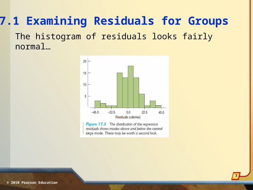
17.1 Examining Residuals for GroupsThe histogram of residuals looks fairly normal…
© 2010 Pearson Education
4
17.1 Examining Residuals for Groups
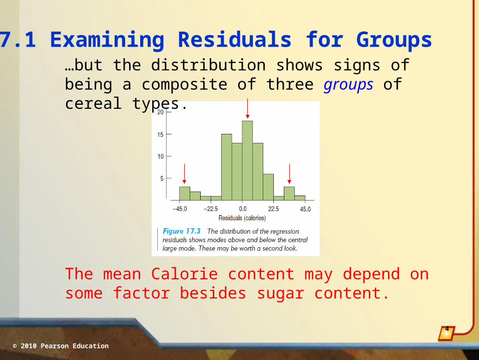
The mean Calorie content may depend on some factor besides sugar content.
…but the distribution shows signs of being a composite of three groups of cereal types.
© 2010 Pearson Education
5
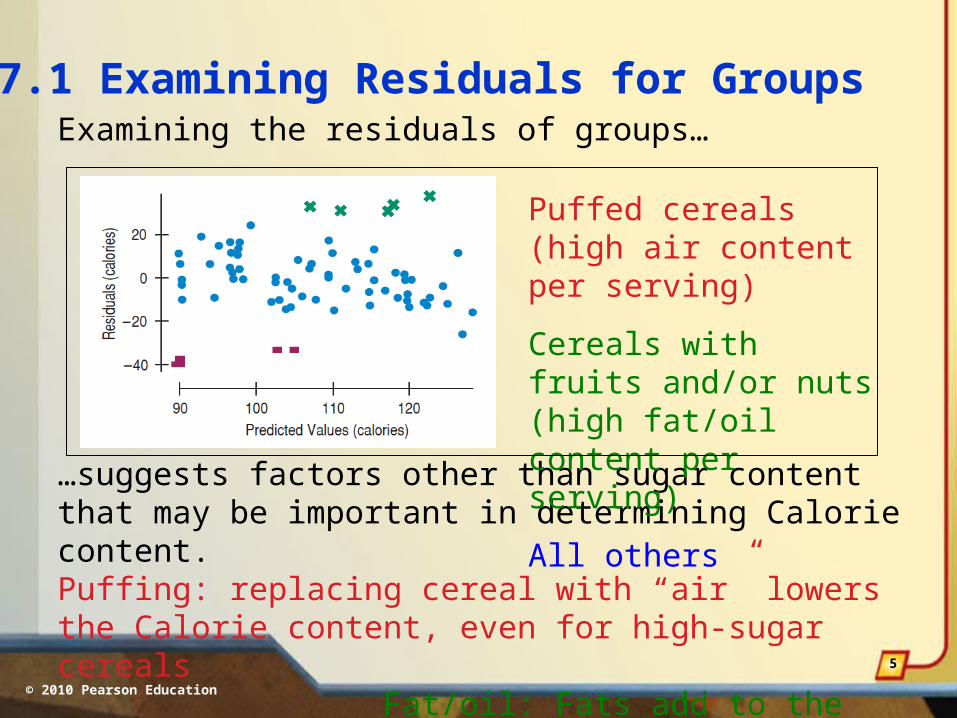
17.1 Examining Residuals for GroupsExamining the residuals of groups…
…suggests factors other than sugar content that may be important in determining Calorie content.Puffing: replacing cereal with “air” lowers the Calorie content, even for high-sugar cereals
Fat/oil: Fats add to the Calorie content, even for low-sugar cereals
Puffed cereals (high air content per serving)
Cereals with fruits and/or nuts (high fat/oil content per serving)
All others
© 2010 Pearson Education
6
17.1 Examining Residuals for GroupsConclusion:
It may be better to report three regressions, one for puffed cereals, one for high-fat cereals, and one for all others.

© 2010 Pearson Education
7
17.2 Extrapolation and PredictionExtrapolating – predicting a y value by extending the regression model to regions outside the range of the x-values of the data.

© 2010 Pearson Education
8
17.2 Extrapolation and PredictionWhy is extrapolation dangerous?
It introduces the questionable and untested assumption that the relationship between x and y does not change.

© 2010 Pearson Education
9
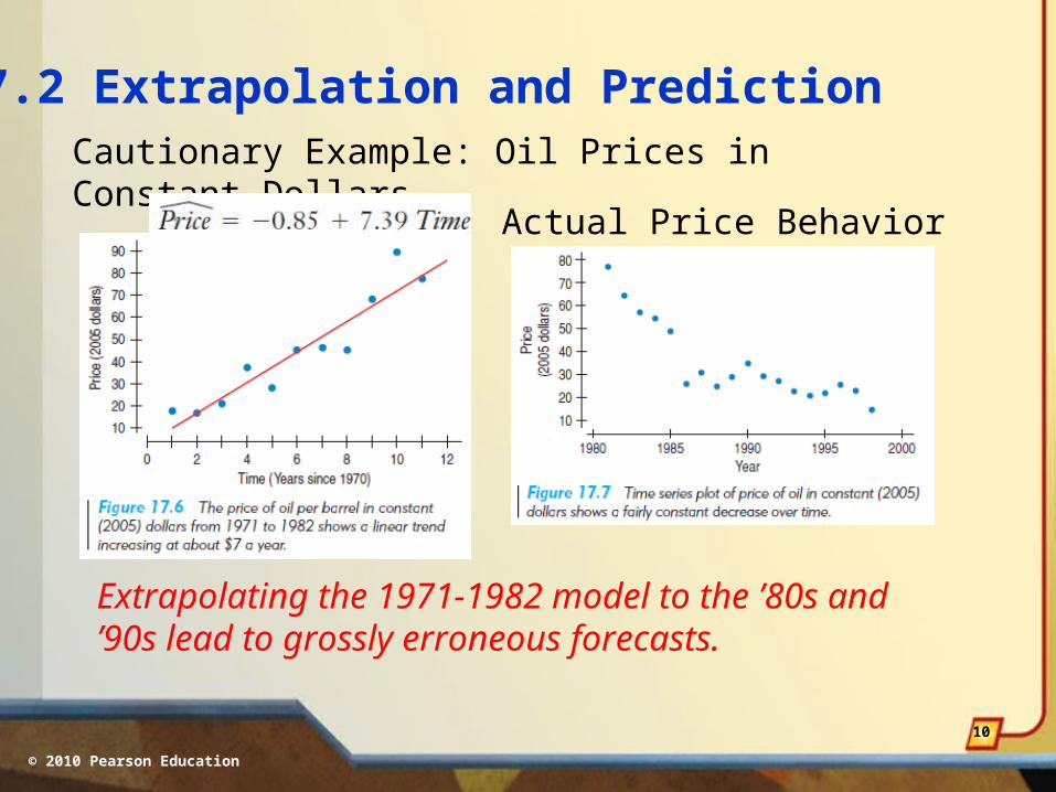
17.2 Extrapolation and PredictionCautionary Example: Oil Prices in Constant Dollars
Model Prediction (Extrapolation):
On average, a barrel of oil will increase $7.39 per year from 1983 to 1998.
© 2010 Pearson Education
10
17.2 Extrapolation and PredictionCautionary Example: Oil Prices in Constant Dollars
Actual Price Behavior
Extrapolating the 1971-1982 model to the ’80s and ’90s lead to grossly erroneous forecasts.

© 2010 Pearson Education
11
17.2 Extrapolation and PredictionRemember: Linear models ought not be trusted beyond the span of the x-values of the data.
If you extrapolate far into the future, be prepared for the actual values to be (possibly quite) different from your predictions.

© 2010 Pearson Education
12
17.3 Unusual and ExtraordinaryObservations
In regression, an outlier can stand out in two ways. It can have…
1). a large residual:
© 2010 Pearson Education
13
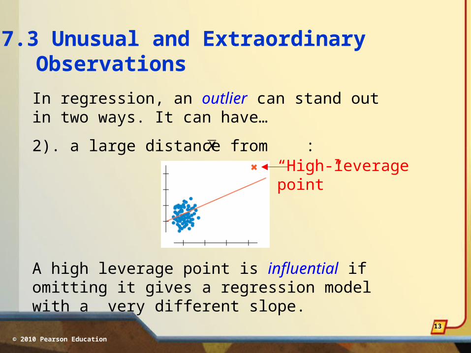
17.3 Unusual and ExtraordinaryObservations
In regression, an outlier can stand out in two ways. It can have…
2). a large distance from : x“High-leveragepoint”
A high leverage point is influential if omitting it gives a regression model with a very different slope.

© 2010 Pearson Education
14
17.3 Unusual and ExtraordinaryObservations
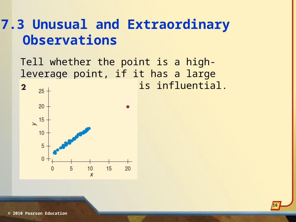
Tell whether the point is a high-leverage point, if it has a large residual, and if it is influential.
© 2010 Pearson Education
15
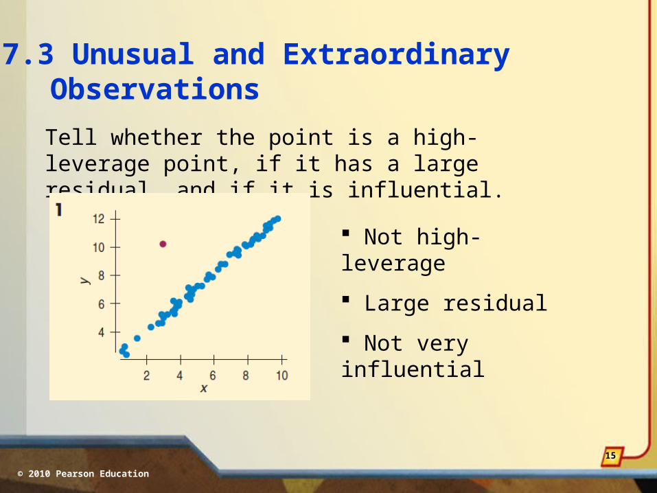
17.3 Unusual and ExtraordinaryObservations
Tell whether the point is a high-leverage point, if it has a large residual, and if it is influential.
Not high-leverage
Large residual
Not very influential
© 2010 Pearson Education
16
17.3 Unusual and ExtraordinaryObservations
Tell whether the point is a high-leverage point, if it has a large residual, and if it is influential.

© 2010 Pearson Education
17
17.3 Unusual and ExtraordinaryObservations
Tell whether the point is a high-leverage point, if it has a large residual, and if it is influential.
High-leverage
Small residual
Not very influential

© 2010 Pearson Education
18
17.3 Unusual and ExtraordinaryObservations
Tell whether the point is a high-leverage point, if it has a large residual, and if it is influential.
© 2010 Pearson Education
19
17.3 Unusual and ExtraordinaryObservations
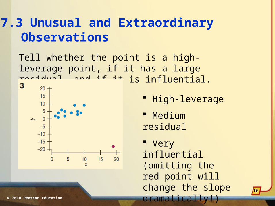
Tell whether the point is a high-leverage point, if it has a large residual, and if it is influential.
High-leverage
Medium residual
Very influential (omitting the red point will change the slope dramatically!)
© 2010 Pearson Education
20
17.3 Unusual and ExtraordinaryObservations
What should you do with a high-leverage point?
Sometimes, these points are important. They can indicate that the underlying relationship is in fact nonlinear.
Other times, they simply do not belong with the rest of the data and ought to be omitted.
When in doubt, create and report two models: one with the outlier and one without.
© 2010 Pearson Education
21
17.3 Unusual and ExtraordinaryObservations
WARNING:
Influential points do not necessarily have high residuals!
So, use scatterplots rather than residual plots to identify high-leverage outliers.
(Residual plots work well of course for identifying high-residual outliers.)
© 2010 Pearson Education
22
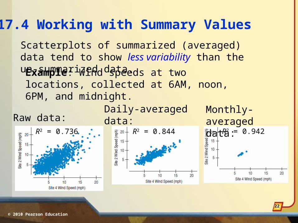
17.4 Working with Summary Values
Scatterplots of summarized (averaged) data tend to show less variability than the un-summarized data.
Example: Wind speeds at two locations, collected at 6AM, noon, 6PM, and midnight.
Raw data:Daily-averageddata:
Monthly-averaged data:
R2 = 0.736 R2 = 0.844 R2 = 0.942

© 2010 Pearson Education
23
17.4 Working with Summary Values
WARNING:
Be suspicious of conclusions based on regressions of summary data.
Regressions based on summary data may look better than they really are!
In particular, the strength of the correlation will be misleading.
© 2010 Pearson Education
24
17.5 Autocorrelation
Time-series data are sometimes autocorrelated, meaning points near each other in time will be related.
First-order autocorrelation:Adjacent measurements are related
Second-order autocorrelation:Every other measurement is related
etc…
Autocorrelation violates the independence condition. Regression analysis of autocorrelated data can produce misleading results.

© 2010 Pearson Education
25
17.5 Autocorrelation
Autocorrelation can sometimes be detected by plotting residuals versus time.
Don’t rely on plots to detect autocorrelation. Rather, use the Durbin-Watson statistic.
© 2010 Pearson Education
26
17.5 Autocorrelation
2
12
2
1
n
t ti
n
tt
e eD
e
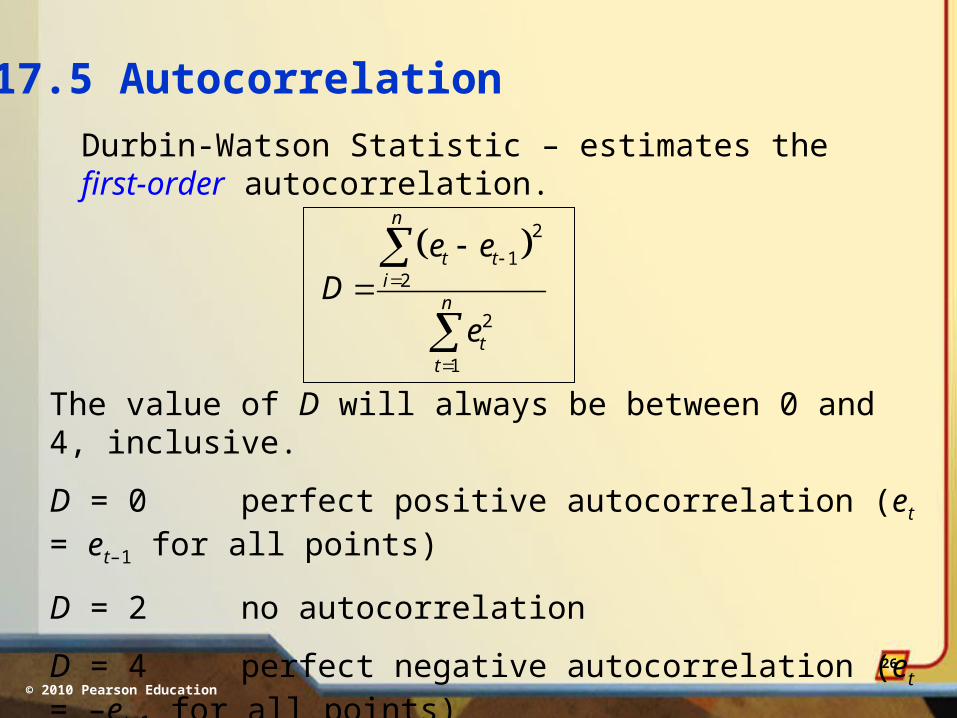
The value of D will always be between 0 and 4, inclusive.
D = 0 perfect positive autocorrelation (et = et–1 for all points)
D = 2 no autocorrelation
D = 4 perfect negative autocorrelation (et = –et–1 for all points)
Durbin-Watson Statistic – estimates the first-order autocorrelation.
© 2010 Pearson Education
27
17.5 Autocorrelation
Whether the calculated Durbin-Watson statistic D indicates significant autocorrelation depends on the sample size, n, and the number of predictors in the regression model, k.
Table W of Appendix C provides critical values for the Durbin-Watson statistic (dL and dU) based on n and k.
© 2010 Pearson Education
28
17.5 Autocorrelation
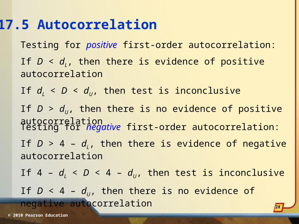
Testing for positive first-order autocorrelation:
If D < dL, then there is evidence of positive autocorrelation
If dL < D < dU, then test is inconclusive
If D > dU, then there is no evidence of positive autocorrelation
Testing for negative first-order autocorrelation:
If D > 4 – dL, then there is evidence of negative autocorrelation
If 4 – dL < D < 4 – dU, then test is inconclusive
If D < 4 – dU, then there is no evidence of negative autocorrelation

© 2010 Pearson Education
29
17.5 Autocorrelation
Dealing with autocorrelation:
Time series methods (Chapter 20) attempt to deal with the problem by modeling the errors.
Or, look for a predictor variable (Chapter 19) that removes the dependence in the residuals.
A simple solution: sample from the time series to minimize first-order autocorrelation (sampling may do nothing to minimize higher-order autocorrelation, though).
© 2010 Pearson Education
30
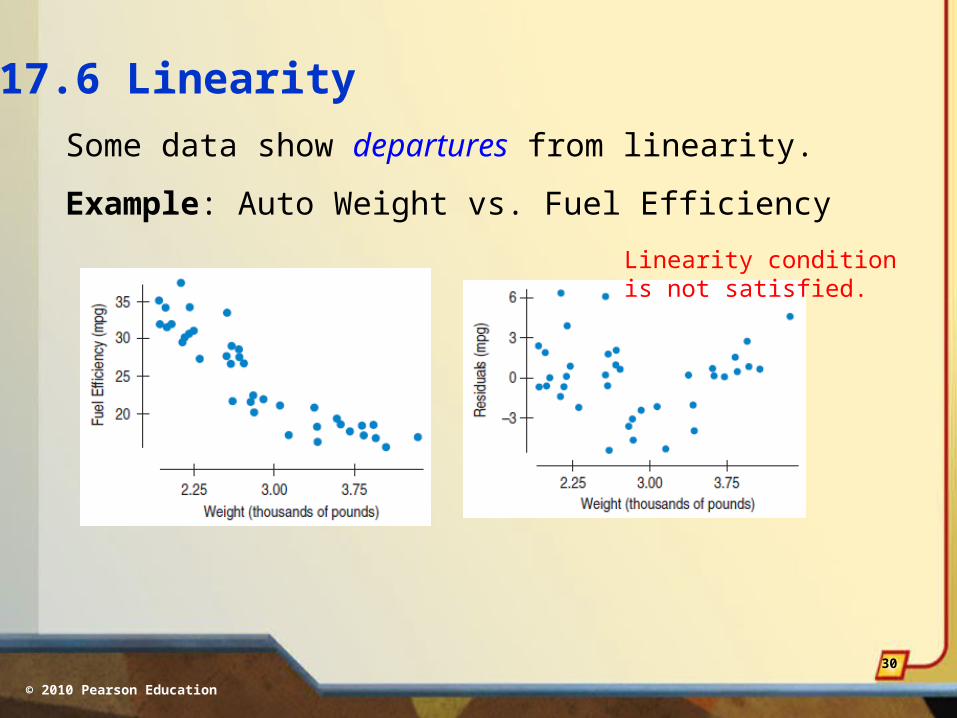
17.6 Linearity
Some data show departures from linearity.
Example: Auto Weight vs. Fuel Efficiency
Linearity condition is not satisfied.
© 2010 Pearson Education
31
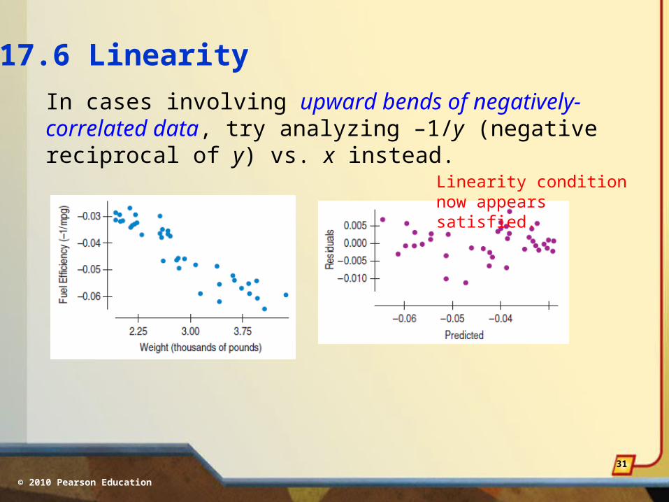
17.6 Linearity
In cases involving upward bends of negatively-correlated data, try analyzing –1/y (negative reciprocal of y) vs. x instead.
Linearity condition now appears satisfied.
© 2010 Pearson Education
32
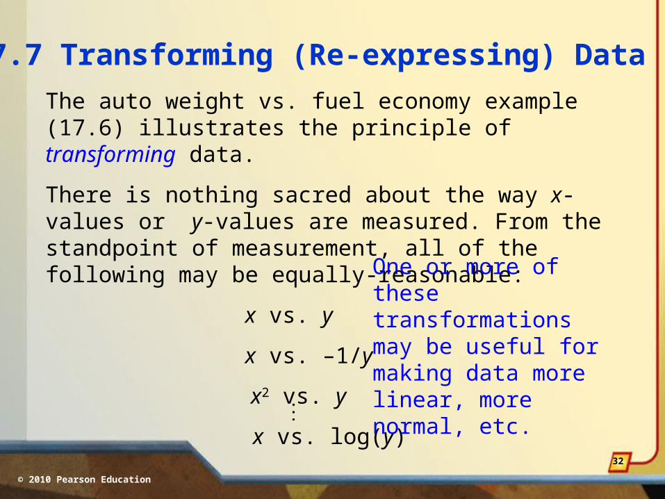
17.7 Transforming (Re-expressing) Data
The auto weight vs. fuel economy example (17.6) illustrates the principle of transforming data.
There is nothing sacred about the way x-values or y-values are measured. From the standpoint of measurement, all of the following may be equally-reasonable:
x vs. y
x vs. –1/y
x2 vs. y
x vs. log(y)
One or more of these transformations may be useful for making data more linear, more normal, etc.
© 2010 Pearson Education
33
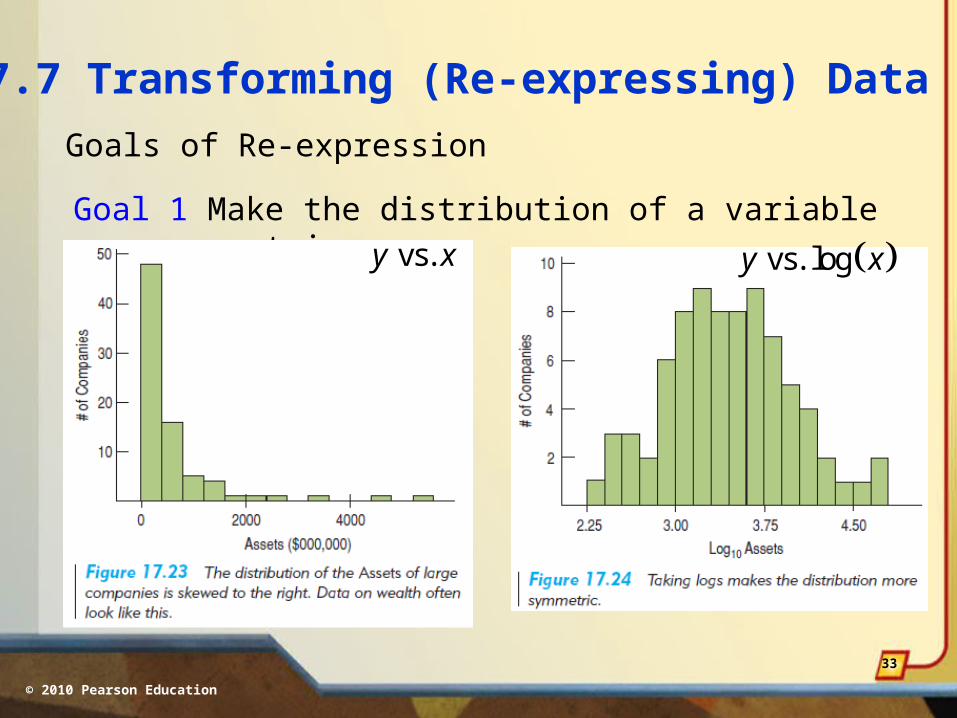
17.7 Transforming (Re-expressing) Data
Goals of Re-expression
Goal 1 Make the distribution of a variable more symmetric.
vs. y x vs. logy x

© 2010 Pearson Education
34
17.7 Transforming (Re-expressing) Data
Goals of Re-expression
Goal 2 Make the spread of several groups more alike.
vs. y x log vs. y x
We’ll see methods later in the book that can be applied only to groups with a common standard deviation.

© 2010 Pearson Education
35
17.7 Transforming (Re-expressing) Data
Goals of Re-expression
Goal 3 Make the form of a scatterplot more nearly linear.
vs. y x log vs. logy x
© 2010 Pearson Education
36
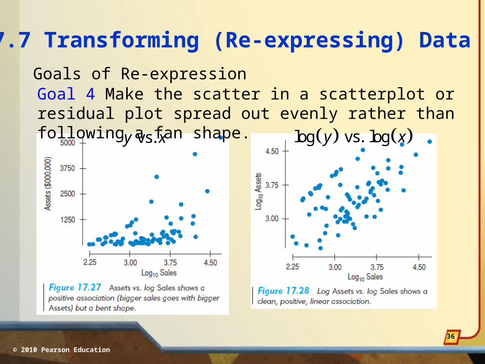
17.7 Transforming (Re-expressing) Data
Goals of Re-expressionGoal 4 Make the scatter in a scatterplot or residual plot spread out evenly rather than following a fan shape.
vs. y x log vs. logy x

© 2010 Pearson Education
37
17.8 The Ladder of Powers
Ladder of Powers – a collection of frequently-useful re-expressions.

© 2010 Pearson Education
38
17.8 The Ladder of Powers
Ladder of Powers – a collection of frequently-useful re-expressions.

© 2010 Pearson Education
39
17.8 The Ladder of Powers
Ladder of Powers – a collection of frequently-useful re-expressions.

© 2010 Pearson Education
40
17.8 The Ladder of Powers
You want to model the relationship between prices for various items in Paris and Hong Kong. The scatterplot of Hong Kong prices vs. Paris prices shows a generally straight pattern with a a small amount of scatter.
What re-expression (if any) of the Hong Kong prices might you start with?

© 2010 Pearson Education
41
17.8 The Ladder of Powers
You want to model the relationship between prices for various items in Paris and Hong Kong. The scatterplot of Hong Kong prices vs. Paris prices shows a generally straight pattern with a a small amount of scatter.
What re-expression (if any) of the Hong Kong prices might you start with?
No re-expression is needed to strengthen the linearity assumption. More information is needed to decide whether re-expression might strengthen the normality assumption or the equal-variance assumption.

© 2010 Pearson Education
42
17.8 The Ladder of Powers
You want to model the population growth of the United States over the past 200 years with a percentage growth that’s nearly constant. The scatterplot shows a strongly upwardly curves pattern.
What re-expression (if any) of the Hong Kong prices might you start with?

© 2010 Pearson Education
43
17.8 The Ladder of Powers
You want to model the population growth of the United States over the past 200 years with a percentage growth that’s nearly constant. The scatterplot shows a strongly upwardly curves pattern.
What re-expression (if any) of the Hong Kong prices might you start with?
Try a “Power 0” (logarithmic) re-expression of the population values. This should strengthen the linearity assumption.

© 2010 Pearson Education
44
What Can Go Wrong? Make sure the relationship is straight enough to fit a regression model. Be alert for extreme residuals and what they have to say about the data.
Be on guard for data that is a composite of values from different groups. If you find data subsets that behave differently, consider fitting a different model to each group.
Beware of extrapolating. Be particularly wary of extrapolating far into the future.
Look for unusual points: points with large residuals and high-leverage points.

© 2010 Pearson Education
45
What Can Go Wrong? Beware of high-leverage points, especially those that are influential.
Consider setting aside outliers and re-running the regression.
Treat unusual points honestly. You must not eliminate points simply to “get a good fit”.
Be alert for autocorrelation. A Durbin-Watson test can be useful for revealing first-order autocorrelation.
© 2010 Pearson Education
46
What Can Go Wrong? Watch out when dealing with data that are summaries. These tend to inflate the impression of the strength of the correlation.
Re-express your data when necessary.

© 2010 Pearson Education
47
What Have We Learned?
Watch out for more than one group hiding in your regression analysis.
The Linearity Condition says that the relationship should be reasonably linear to fit a regression. The satisfaction of this condition is best assessed after performing the regression and examining the residuals.
The Outlier Condition refers to two kinds of points: those with large residuals and those with high leverage. It’s a good idea to perform the regression analysis both with them and without them.