Chapter 15 Dynamic Programming Lee, Hsiu-Hui Ack: This presentation is based on the lecture slides...

Chapter 15

Dynamic Programming Lee, Hsiu-Hui

Ack: This presentation is based on the lecture slides from Hsu, Lih-Hsing, as well as various materials from the web.

20071207 chap15 Hsiu-Hui Lee 2

Introduction

• Dynamic programmingDynamic programming is typically applied to optimization problems.

• In such problem there can be many solutions. Each solution has a value, and we wish to find a solution with the optimal value.


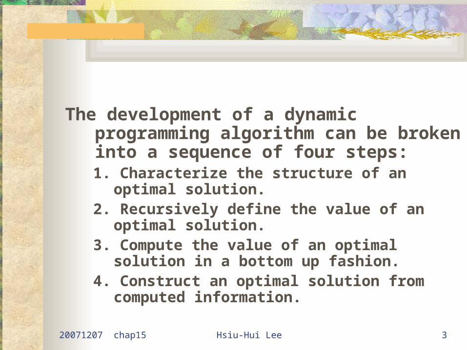
The development of a dynamic programming algorithm can be broken into a sequence of four steps:1. Characterize the structure of an optimal solution.2. Recursively define the value of an optimal solution.3. Compute the value of an optimal solution in a

bottom up fashion.4. Construct an optimal solution from computed

information.


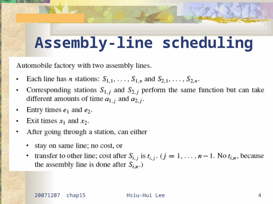
Assembly-line scheduling


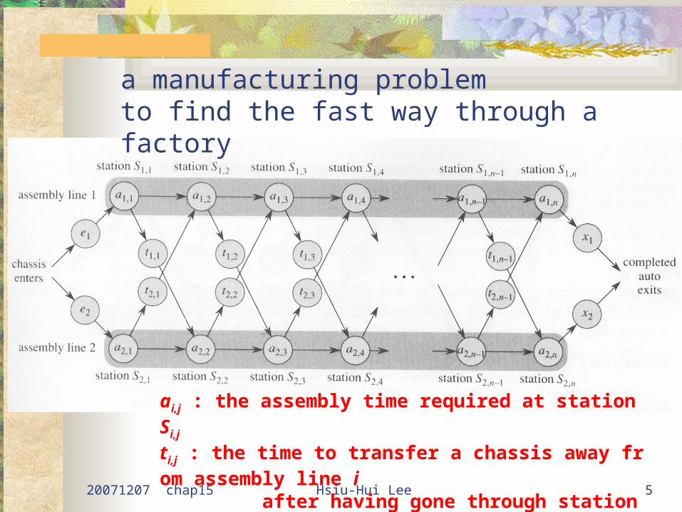
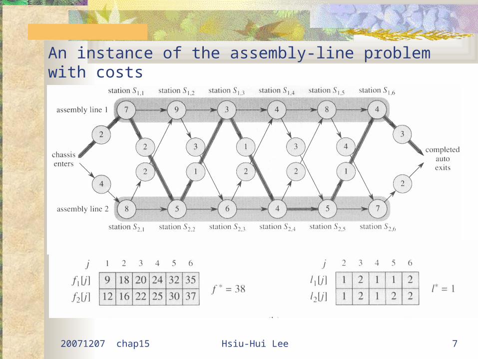
a manufacturing problem to find the fast way through a factory

ai,j : the assembly time required at station Si,j

ti,j : the time to transfer a chassis away from assembly line i after having gone through station Si,j


An instance of the assembly-line problem with costs


Step 1: The structure of the fastest way through the factory


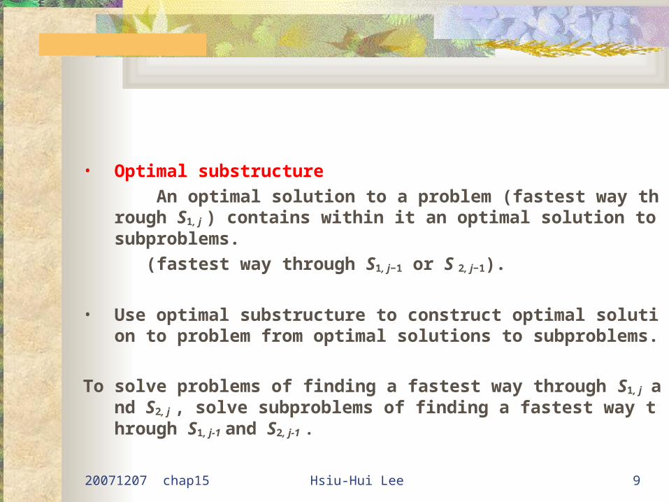
• Optimal substructure

An optimal solution to a problem (fastest way through S1, j ) contains within it an optimal solution to subproblems.

(fastest way through S1, j−1 or S 2, j−1).

• Use optimal substructure to construct optimal solution to problem from optimal solutions to subproblems.

To solve problems of finding a fastest way through S1, j and S2, j , solve subproblems of finding a fastest way through S1, j-1 and S2, j-1 .


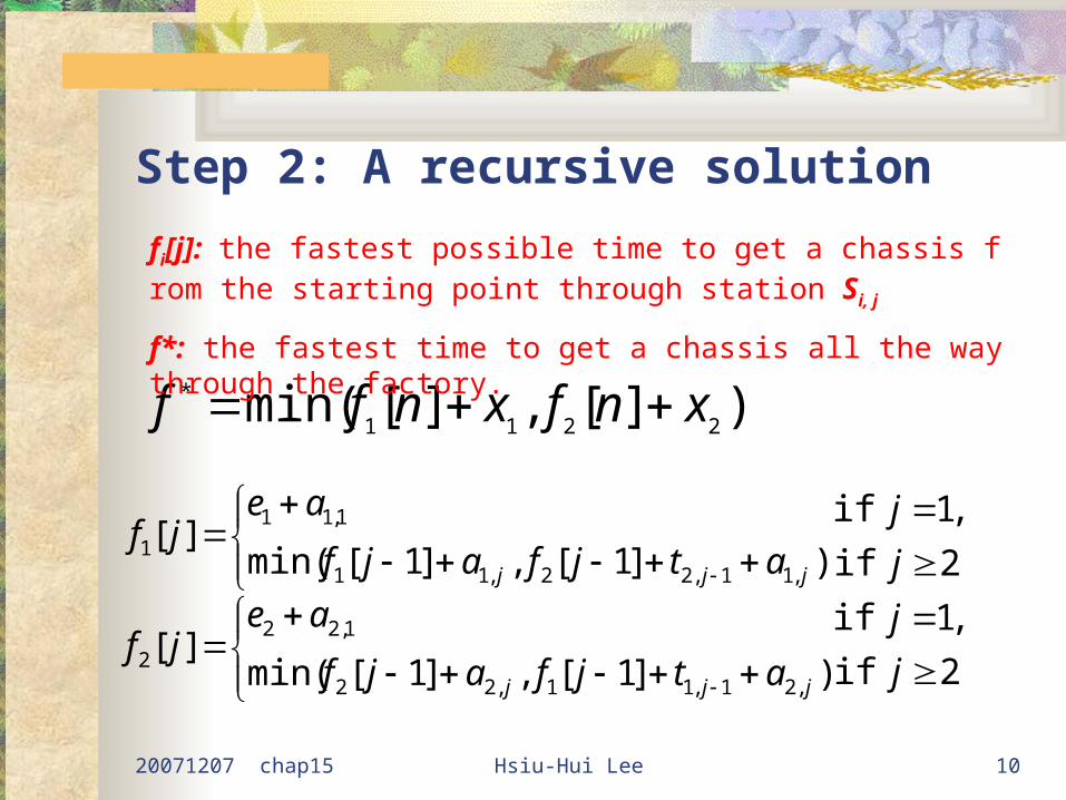
Step 2: A recursive solution

)][,][min(2211

* xnfxnff

2if

,1if

2if

,1if

)]1[,]1[min(][

)]1[,]1[min(][

,21,11,22

1,22

2

,11,22,11

1,11

1

j

j

j

j

atjfajf

aejf

atjfajf

aejf

jjj

jjj

fi[j]: the fastest possible time to get a chassis from the starting point through station Si, j

f*: the fastest time to get a chassis all the way through the factory.


• li [ j ] = line # (1 or 2) whose station j − 1 is used in fastest way through Si, j .

• Sli [ j ], j−1 precedes Si, j .• Defined for i = 1,2 and j = 2, . . . , n.• l∗ = line # whose station n is used.


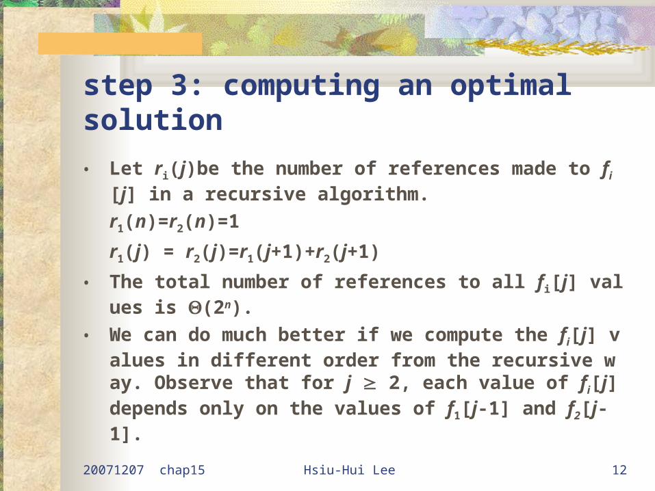
step 3: computing an optimal solution

• Let ri(j)be the number of references made to fi[j] in a recursive algorithm.

r1(n)=r2(n)=1

r1(j) = r2(j)=r1(j+1)+r2(j+1)

• The total number of references to all fi[j] values is (2n).

• We can do much better if we compute the fi[j] values in different order from the recursive way. Observe that for j 2, each value of fi[j] depends only on the values of f1[j-1] and f2[j-1].


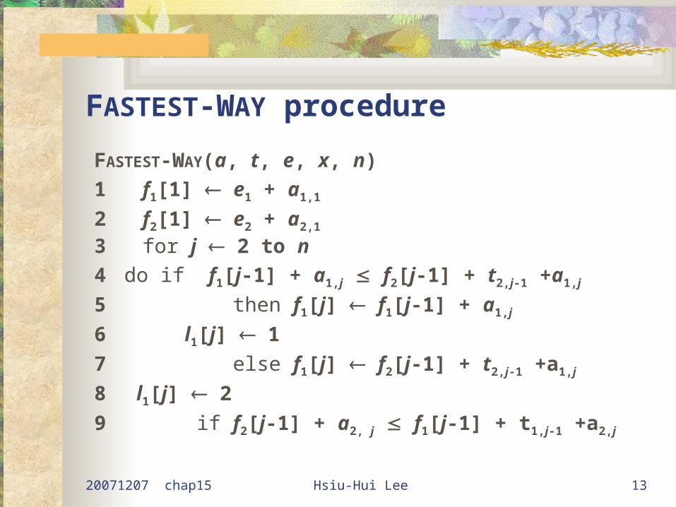
FASTEST-WAY procedure

FASTEST-WAY(a, t, e, x, n)

1 f1[1] e1 + a1,1

2 f2[1] e2 + a2,1

3 for j 2 to n

4 do if f1[j-1] + a1,j f2[j-1] + t2,j-1 +a1,j

5 then f1[j] f1[j-1] + a1,j

6 l1[j] 1

7 else f1[j] f2[j-1] + t2,j-1 +a1,j

8 l1[j] 2

9 if f2[j-1] + a2, j f1[j-1] + t1,j-1 +a2,j


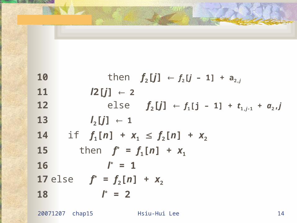
10 then f2[j] f2[j – 1] + a2,j

11 l2[j] 2

12 else f2[j] f1[j – 1] + t1,j-1 + a2,j

13 l2[j] 1

14 if f1[n] + x1 f2[n] + x2

15 then f* = f1[n] + x1

16 l* = 1

17 else f* = f2[n] + x2

18 l* = 2


step 4: constructing the fastest way through the factory

PRINT-STATIONS(l, l*, n)1 i l*2 print “line” i “,station” n3 for j n downto 2

4 do i li[j]

5 print “line” i “,station” j – 1

output

line 1, station 6

line 2, station 5

line 2, station 4

line 1, station 3

line 2, station 2

line 1, station 1


15.2 Matrix-chain multiplication

• A product of matrices is fully parenthesized if it is either a single matrix, or a product of two fully parenthesized matrix product, surrounded by parentheses.


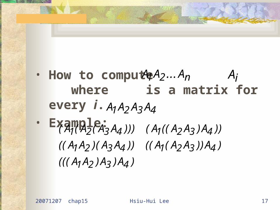
• How to compute where is a matrix for every i.

• Example:

A A An1 2 ... Ai

A A A A1 2 3 4

( ( ( ))) ( (( ) ))

(( )( )) (( ( )) )

((( ) ) )

A A A A A A A A

A A A A A A A A

A A A A

1 2 3 4 1 2 3 4

1 2 3 4 1 2 3 4

1 2 3 4


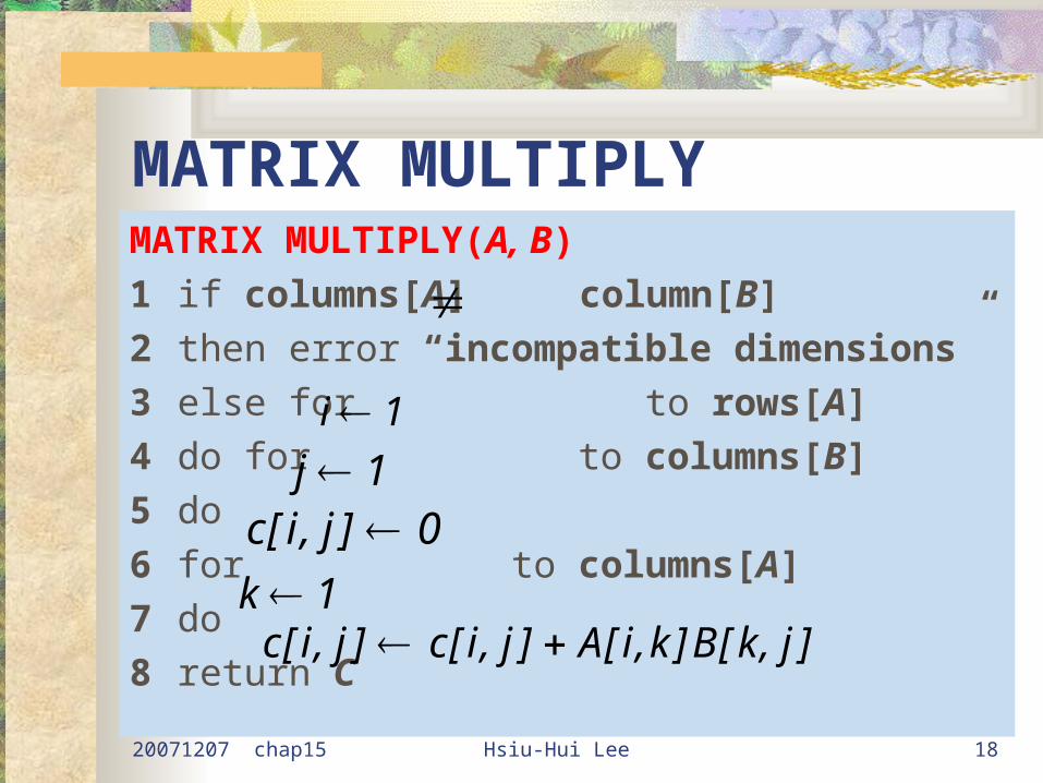
MATRIX MULTIPLY MATRIX MULTIPLY(A, B)

1 if columns[A] column[B]

2 then error “incompatible dimensions”

3 else for to rows[A]

4 do for to columns[B]

5 do

6 for to columns[A]

7 do

8 return C

i 1

j 1c i j[ , ] 0

k 1c i j c i j A i k B k j[ , ] [ , ] [ , ] [ , ]


Complexity:

Let A be a matrix

B be a matrix.

Then the complexity is

p qq r

p q r


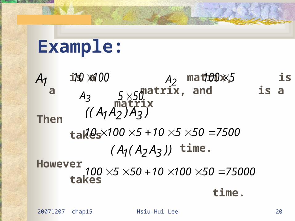
Example:

is a matrix, is a matrix, and is a matrix

Then

takes time.

However

takes time.

A1 10 100 A2 100 5A3 5 50(( ) )A A A1 2 3

10 100 5 10 5 50 7500

( ( ))A A A1 2 3

100 5 50 10 100 50 75000


The matrix-chain multiplication problem: • Given a chain of n

matrices, where for i=0,1,…,n, matrix Ai has dimension pi-1pi, fully parenthesize the product in a way that minimizes the number of scalar multiplications.

nAAA ,...,, 21

A A An1 2 ...


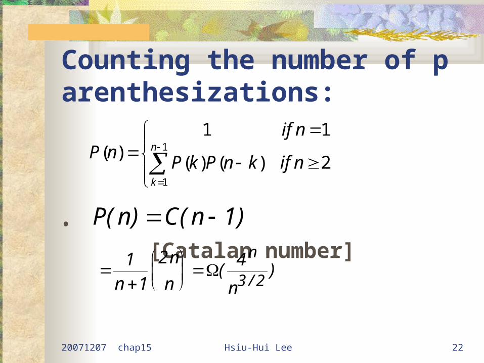
Counting the number of parenthesizations:

• [Catalan number]

2)()(

11)( 1

1

nifknPkP

nifnP n

k

P n C n( ) ( ) 1

11

2 43 2n

n

n n

n( )

/


Step 1: The structure of an optimal parenthesization

(( ... )( ... ))A A A A A Ak k k n1 2 1 2

Optimal

Combine


Step 2: A recursive solution

• Define m[i, j]= minimum number of scalar multiplications needed to compute the matrix

• goal m[1, n]•

A A A Ai j i i j.. .. 1

m i j[ , ]

jipppjkmkim

ji

jkijki }],1[],[{min

0

1

Step 3: Computing the optimal costs


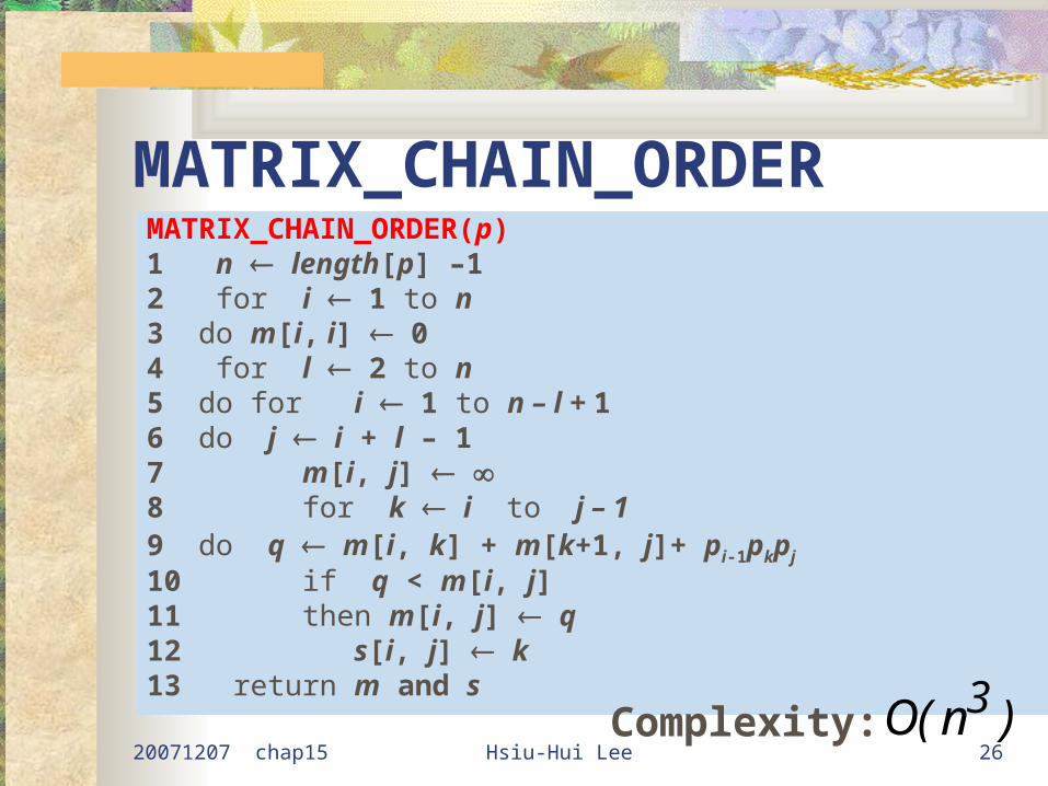
MATRIX_CHAIN_ORDER MATRIX_CHAIN_ORDER(p)1 n length[p] –1 2 for i 1 to n3 do m[i, i] 04 for l 2 to n5 do for i 1 to n – l + 16 do j i + l – 1 7 m[i, j] 8 for k i to j – 1 9 do q m[i, k] + m[k+1, j]+ pi-1pkpj

10 if q < m[i, j]11 then m[i, j] q12 s[i, j] k13 return m and s

Complexity: O n( )3


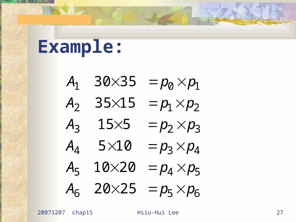
Example:

656

545

434

323

212

101

2520

2010

105

515

1535

3530

ppA

ppA

ppA

ppA

ppA

ppA


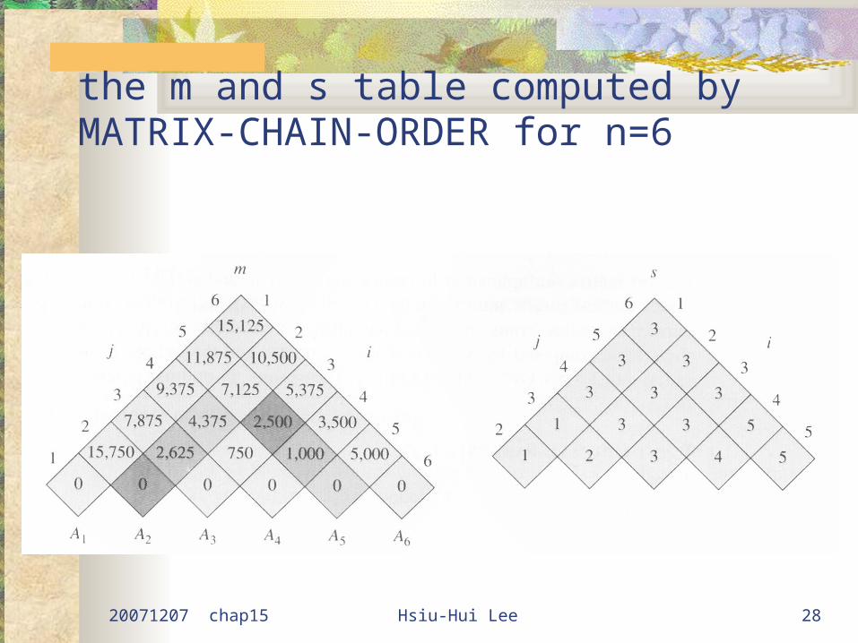
the m and s table computed by MATRIX-CHAIN-ORDER for n=6


m[2,5]=

min{

m[2,2]+m[3,5]+p1p2p5=0+2500+351520=13000,

m[2,3]+m[4,5]+p1p3p5=2625+1000+35520=7125,

m[2,4]+m[5,5]+p1p4p5=4375+0+351020=11374

}

=7125

Step 4: Constructing an optimal solution


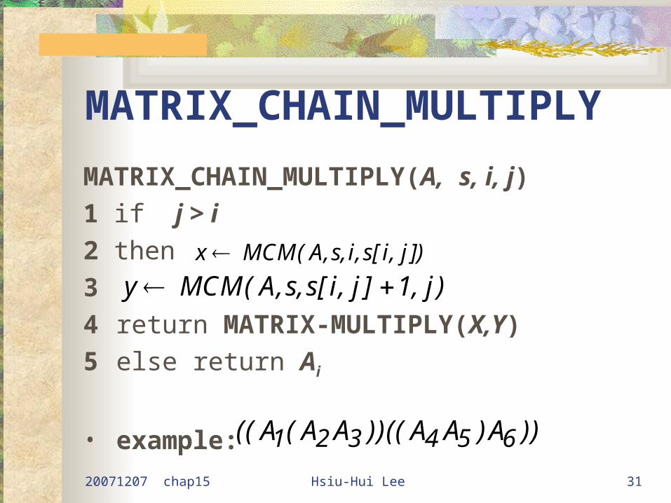
MATRIX_CHAIN_MULTIPLY

MATRIX_CHAIN_MULTIPLY(A, s, i, j)

1 if j > i

2 then

3

4 return MATRIX-MULTIPLY(X,Y)

5 else return Ai

• example: (( ( ))(( ) ))A A A A A A1 2 3 4 5 6

x MCM A s i s i j ( , , , [ , ])

y MCM A s s i j j ( , , [ , ] , )1

Chapter 15 Dynamic Programming Lee, Hsiu-Hui Ack: This presentation is based on the lecture slides...

Documents

Transcript of Chapter 15 Dynamic Programming Lee, Hsiu-Hui Ack: This presentation is based on the lecture slides...