Chapter 14web.stanford.edu/group/fayer/lectures/R19/Chapter14R19.pdf · Density Matrix State of a...

Chapter 14

Density MatrixState of a system at time t: ( )n

nt C t n orthonormal basis setn

2( ) 1nn

C t normalizedt

Density Operator

( )t t t

We’ve seen this before, as a “projection operator”

) (

( )ij t i t

t t

j

i j

Can find density matrix in terms of the basis set nMatrix elements of density matrix:

Contains time dependentphase factors.

Copyright – Michael D. Fayer, 2018

Two state system:

1 2( ) 1 ( ) 2t C t C t

12 1 2t t *

12 1 2C C

21 2 1t t *

21 2 1C C

22 2 2t t *

22 2 2C C

Calculate matrix elements of 2×2 density matrix:

11 1 1t t

* *1 2 1 21 1 2 1 2 1C C C C

*11 1 1C C

Time dependent phasefactors cancel. Alwayshave ket with its complexconjugate bra.

* *1 2( ) 1 ( ) 2t C t C t


In general:

*( )ij i jt C C

*

( )

( ) ( )

ii

i ji j

t C t i

t t C t i j C t

*

( )

( ) ( )k lk l

ij t

i C

i t t j

t k l C t j

ij density matrix element


2×2 Density Matrix:

* *1 1 1 2

* *2 1 2 2

( )C C C C

tC C C C

*2 2

*1 1 Probability of finding system in state

Probability of finding system in state 2

1

C

C

C

C

Diagonal density matrix elements probs. of finding system in various statesOff Diagonal Elements “coherences”

2Since ( ) 1nn

C t ( ) 1Tr t trace = 1 for any

dimension(trace – sum of diagonal matrix elements)

*ij ji

And


( )d tdt

Time dependence of ( )t

( )d t d dt t t tdt d t d t

product rule

Using Schrödinger Eq. for time derivatives of & t t

d t

i H t

ddt

ti t H

dt

1

1

d tH t

dt id t

t Hdt i


( ) 1 1( ) ( )d t

H t t t t t H tdt i i

( ) 1 ( ) ( )d t

H t t t t t H tdt i

1 ( ), ( )H t ti

Substituting:

density operator

Therefore:

( ) ( ), ( )i t H t t

The fundamental equation of the density matrix representation.


( ) ( ), ( )it H t t

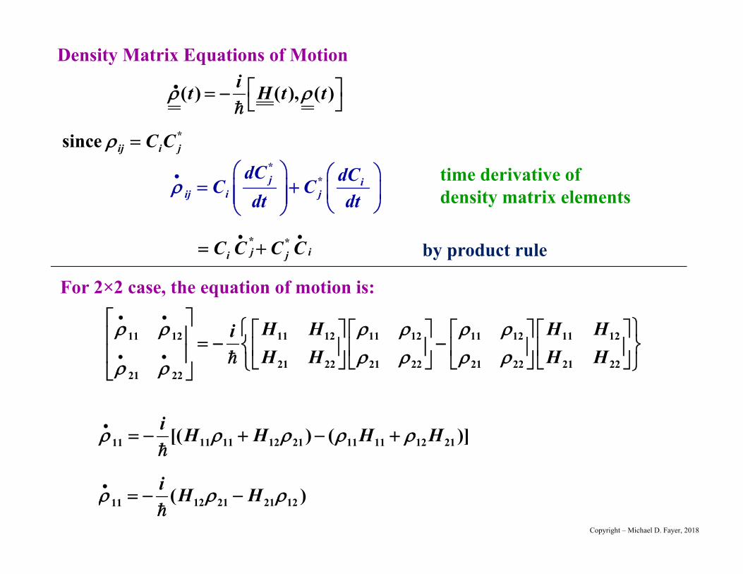
Density Matrix Equations of Motion

*since ij i jC C *

*j ii jij

dC dCC Cdt dt

* *j ii jC C C C

by product rule

For 2×2 case, the equation of motion is:

11 12 11 12 11 12 11 1211 12

21 22 21 22 21 22 21 2221 22

H H H HiH H H H

time derivative of density matrix elements

12 21 21 1211 ( )i H H

11 11 12 21 11 11 12 2111 [( ) ( )]i H H H H


11 12 11 12 11 12 11 1211 12

21 22 21 22 21 22 21 2221 22

H H H HiH H H H

11 22 12 22 11 1212 ( ) ( )i H H H

11 12 12 22 11 12 12 2212 ( ) ( )i H H H H


12 21 21 1211 22 ( )i H H

*11 22 12 22 11 1212 21 ( ) ( )i H H H

Equations of Motion – from multiplying of matrices for 22:

11 22 1 (trace of = 1)

12 21*

for 2x2 because

for any dimension

In many problems:

0 ( )IH H H t

timeindependent

timedependent

e.g., Molecule in a radiation field:

0 molecular HamiltonianH ( ) radiation field interaction (I) with moleculeIH t

0Natural to use basis set of H

0 nH n E n (orthonormal)(time dependent phase factors)

( )nn

t C t n 0Eigenkets of H

Write as:t


For this situation:

( ) ( ), ( )Iit H t t

time evolution of density matrix elements, Cij(t), depends only on ( )IH t

time dependent interaction term

See derivation in book – and lecture slides.Like first steps in time dependent perturbation theory

before any approximations.

In absence of , only time dependence from time dependent phase factorsfrom . No changes in magnitudes of coefficients Cij .

IH0H


Time Dependent Two State Problem Revisited:

Previously treated in Chapter 8 with Schrödinger Equation.

0Basis set 1 , 2 degenerate eigenkets of H

No IH0 01 1 1H E

0 02 2 2H E

Interaction IH1 2IH

2 1IH of Ch. 8

00IH

The matrix IH

Because degenerate states, time dependent phase factors cancel in off-diagonal matrix elements – special case.In general, the off-diagonal elements have time dependent phase factors.


( ) ( ), ( )I

it H t t Use

11 12 11 12

2 1 22 21 22

0 00 0

i

12 21 11 22

11 22 12 21

( ) ( )( ) ( )

i

Multiplying matrices and subtracting gives

Equations of motion of density matrix elements:

12 2111 ( )i

12 2122 ( )i

Probabilities

11 2212 ( )i

11 2221 ( )i

Coherences

00IH

11 21 11 1211

21 12 12 21

[(0 ) ( 0 )]( ) ( )

ii i


Using

11 12 21( )i

11 12 21( )i

Take time derivative

211 2211 2 ( )

Using Tr = 1, i.e., 11 22 1

22 11Then 1

2 21111 2 4 and

222 sin ( )t

/From Ch. 8

Same result as Chapter 8 except obtained probabilities directly. No probability amplitudes.

12 21Substitute &

11 2212 ( )i 11 2221 ( )i

For initial condition at t = 0. 11 1

211 cos ( )t

2

2 2 2 2 2 2

2 2

2 2 2 2 2

2 2 2

cos ( )/ 2 cos( )sin( )cos ( )/ 2 (sin ( ) cos ( ))

but sin ( ) 1 cos ( )then cos ( )/ 2 (1 2cos ( ))

2 4 cos ( )

d t dt t td t dt t t

t td t dt t

t


Can get off-diagonal elements

*Since ij ji

21 sin(2 )2i t

11 2212 ( )i

Substituting:2 2

12 (cos sin )i t t

2 212 cos sini t t dt

12 sin(2 )2i t

2

2

cos (1/2) (1/ 4)sin 2

sin (1/2) (1/ 4)sin 2

xdx x x

xdx x x


*( ) ( ) ( )ij i jt C t C t

*

( )

( ) ( )

ii

i ji j

t C t i

t t C t i j C t

*

*

*

( )

( )

( )

( ) ( )

)

( )

(

k lk

ij

i j

i j

l

C t

i C t k l C

C t i i C

t i t t j

C t

t j

t j j

ij density matrix element

Density matrix elements have no time dependent phase factors.

time dependent phase factor in ket, butits complex conjugate is in bra. Productis 1. Kets and bras normalized, closedbracket gives 1.

Time dependent coefficient, but no phase factors.


Can be time dependent phase factors in density matrix equation of motion.

( ) ( ), ( )it H t t

2221

1211

HHHH

H1

2

/

/

1 1

2 2

iE ts

iE ts

e

e

s – spatial

1 1/ /11 1 1 1 1 1 1iE t iE t

s ss sH H H e e H no time dependent phasefactor

1 2 1 2/ / ( ) /12 1 2 1 2 1 2iE t iE t i E E t

s ss sH H H e e H e

time dependent phase factorif E1 ≠ E2.

Therefore, in general, the commutator matrix,

( ), ( )H t t

will have time dependent phase factors if E1 ≠ E2.

For two levels, but the same in any dimension.

when you multiply it out,


Expectation Value of an Operator

A t A t

Complete orthonormal basis set j

( )jj

t C t j

ijA i A j

Matrix elements of A

Derivation in book and see lecture slides

( )A Tr t A

Expectation value of A is trace of the product of density matrix with the operator matrix .A

Important: carries time dependence of coefficients.( )t

Time dependent phase factors may occur in off-diagonal matrix elements of A.Copyright – Michael D. Fayer, 2018

Example: Average E for two state problem

E H Tr H

0 I

EH H H

E

2 2(cos sin ) (sin 2 sin 2 )2

iH E t t t t

E

11 12

21 22

ETr H Tr

E

11 12 21 22

11 22 12 21( ) ( )E E

E

Only need to calculate thediagonal matrix elements.

Time dependent phase factors cancel because degenerate. Special case. In general have time dependent phase factors.

21 sin(2 )2i t 12 sin(2 )

2i t 2

11 cos ( )t 222 sin ( )t

EE

E

E = 0


Working with basis set of eigenkets of time independent piece of Hamiltonian,H0, the time dependence of the density matrix depends only on the timedependent piece of the Hamiltonian, HI.

Total Hamiltonian

0 ( )IH H H t

0H

0 nH n E n

time independent

nUse as basis set.

( )nn

t C t n

Proof that only need consider

( ) ( ), ( )Iit H t t

when working in basis set of eigenvectors of H0.


Time derivative of density operator (using chain rule)

d dt t t td t d t

(A)

1 1( ) ( )H t t t t t H ti i

0 01 1 1 1

I IH t t H t t t t H t t Hi i i i

Use Schrödinger Equation and its complex conjugate

(B)

Substitute expansion into derivative terms in eq. (A).( )nn

t C t n*

n nn n

d dC n t t C nd t d t

* *

n n n nn n n n

d dC n t C n t t C n t C nd t d t

(C)

(B) = (C)Copyright – Michael D. Fayer, 2018

Using Schrödinger Equation

01

nn

dC n H td t i

*0

1n

n

dC n t Hd t i

t

tRight multiply top eq. by .

Left multiply bottom equation by .

Gives

01

nn

dC n t H t td t i

*0

1n

n

dt C n t t Hd t i

Using these see that the 1st and 3rd termsin (B) cancel the 2nd and 4th terms in (C).

0 01 11 1

I IH t t t t Hi i

H t t t t Hi i

**n nn n

n nn n

C n t td dC n t t C nd t t

C nd

(B)

(C)


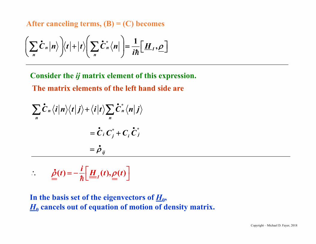
* 1 ,n n In n

C n t t C n Hi

After canceling terms, (B) = (C) becomes

Consider the ij matrix element of this expression.

*n n

n nC i n t j i t C n j

**

i jj iC C C C

ij

The matrix elements of the left hand side are

( ) ( ), ( )I

it H t t

In the basis set of the eigenvectors of H0,H0 cancels out of equation of motion of density matrix.


Expectation value

A t A t

j

( )jj

t C t j

complete orthonormal basis set.

ijA i A j

*i j

i jt A t C i A C j

Matrix elements of A

*

,

( ) ( )i ji j

C t C t i A j

t A t ( )A Tr t AProof that =


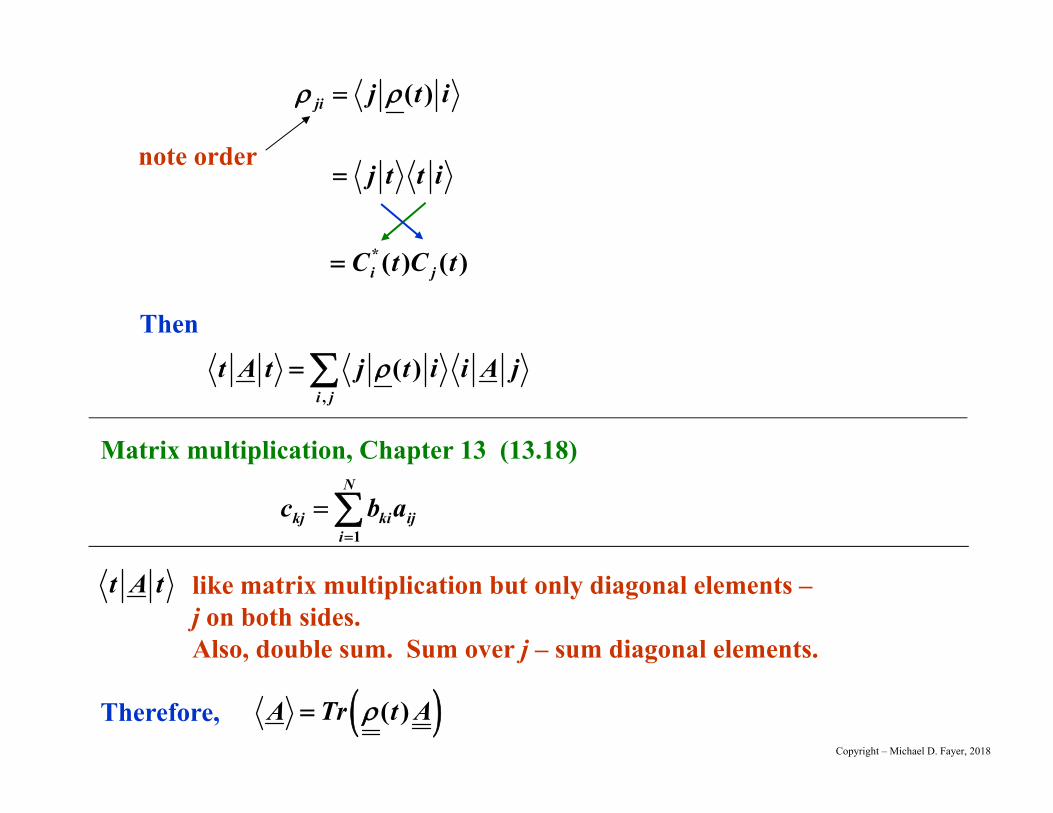
( )ji j t i

j t t i

*( ) ( )i jC t C t

,

( )i j

t A t j t i i A j

note order

Then

Matrix multiplication, Chapter 13 (13.18)

1

N

kj ki iji

c b a

t A t like matrix multiplication but only diagonal elements –j on both sides.Also, double sum. Sum over j – sum diagonal elements.

Therefore, ( )A Tr t ACopyright – Michael D. Fayer, 2018

radiationfield

Coherent Coupling by of Energy Levels by Radiation Field

Two state problem

0 1

0 1

2 electronic states 2 vibrational states

S SV V

In general, if radiation field frequency is near E, and other transitionsare far off resonance, can treat as a 2 state system.

NMR – 2 spin states, magnetic transition dipole


0E

1

2

1 0E

2 0E

0 11 1H E

0 22 2H E

Molecular Eigenstates as Basis

Interaction due to application of optical field (light) on or near resonance.

12 0( ) cos( )IH t e x E t

2

0

1 transition dipole operator

pola

rized li amplit

gdeht

u

e x

Ex


Take real (doesn’t change results)

Define Rabi Frequency, 11 0E

Then 011 ( ) 2 cos( ) i t

IH t t e

012 ( ) 1 cos( ) i t

IH t t e

( ) matrix:I

H t0

0

1

1

0 cos( )( )

cos( ) 0

i t

i tI

t eH t

t e

1201 ( ) 2 cos( ) 1 2IH t E t e x

couples statesIH

0*0 cos2 ( ) 1 ( )I

i tH E et t

1 2/ /0 1 2 012cos( ) 1 2 0iE t iE tE t e e x e E E

00 cos( ) i tE t e is value of

transition dipole bracket,Note – time independent

kets. No phase factors. Have takenphase factors out.

take out time dependent phase factors


Use ( ) ( ), ( )I

it H t t

11 12

21 22

0 0

0

0

0 0

1 12 1 11 221

1 12 2

2

1 11 22 1

cos( ) ( )

co

cos( )

s( ) ( os) c ( )

i t i t

i t

i t

i t i t

i t e e

i t e

t e

t e

i

i e

Blue diagonalRed off-diagonal

1 2( ) 1 ( ) 2t C t C t General state of system

0

0

0

0

11 121

2 1 221

11 12 1

21 22 1

0 cos( )cos( ) 0

0 cos( )cos( ) 0

i t

i t

i t

i t

t eit e

t et e


Equations of Motion of Density Matrix Elements

0 01 12 2111 cos( ) i t i ti t e e

0 01 12 2122 cos( ) i t i ti t e e

01 11 2212 cos( ) ( )i ti t e

01 11 2221 cos( ) ( )i ti t e

*12 21

*

12 21

11 22 11 22 1

Treatment exact to this point (expect for dipole approx. in ).


Rotating Wave Approximation

1cos( )2

i t i tt e e

Put this into equations of motionWill have terms like

0 0( ) ( ) and i t i te e

0But

Terms with off resonance Don’t cause transitions0 0( ) 2

Looks like high frequency Stark Effect Bloch – Siegert Shift

Small but sometimes measurable shift in energy.

Drop these terms!


With Rotating Wave Approximation

Equations of motion of density matrix

0 0( ) ( )112 2111 2

i t i ti e e

0 0( ) ( )112 2122 2

i t i ti e e

0( )111 2212 ( )

2i ti e

0( )111 2221 ( )

2i ti e

These are theOptical Bloch Equations for optical transitionsor just the Bloch Equations for NMR.

1 1NMR - m H


H1 – oscillating magnetic field of applied RF.m – magnetic transition dipole.

Consider on resonance case = 0

Equations reduce to

112 2111 2

i

112 2122 2

i

111 2212 ( )

2i

111 2221 ( )

2i

These are IDENTICAL to the degenerate time dependent 2 state problemwith = 1/2.

0 0( ) ( )112 2111 2

i t i ti e e

0 0( ) ( )112 2122 2

i t i ti e e

0( )111 2212 ( )

2i ti e

0( )111 2221 ( )

2i ti e

All of the phase factors = 1.


On resonance coupling to time dependent radiation field induces transitions.

Looks identical to time independentcoupling of two degenerate states.

0 In effect, the on resonance radiation field “removes” energy differences andtime dependence of field.

2 111 cos ( )

2t

2 122 sin ( )

2t

12 1sin( )2i t

21 1sin( )2i t

Start in ground state, 1 11 22 12 211; 0, 0, 0

0E

2

1

22

11

Then

populations coherences

at t = 0.


2 111 cos ( )

2t 2 1

22 sin ( )2

t

1 0 Rabi FrequencyE Recall

111 22 1,0t

This is called a pulse inversion, all population in excited state.

populations

11 221 0 ,.52

0.5t

This is called a /2 pulse Maximizes off diagonal elements 12, 21

As t is increased, populationoscillates between ground and excited state at Rabi frequency.

Transient NutationCoherent Coupling

2 4 6 8

0.2

0.4

0.6

0.8

1

t

22

–ex

cite

d st

ate

prob

. pulse

2 pulse Copyright – Michael D. Fayer, 2018

Off Resonance Coherent Coupling0

1/ 22 21 Effective Fielde Define

For same initial conditions:

Solutions of Optical Bloch Equations

221

11 21 sin ( /2)ee

t

221

22 2 sin ( /2)ee

t

2112 2 sin( ) sin ( /2)

2i te

e ee

i t t e

2121 2 sin( ) sin ( /2)

2i te

e ee

i t t e

Oscillations Faster eMax excited state probability:

2max 122 2

e

(Like non-degenerate time dependent 2-state problem)

11 22 12 211; 0, 0, 0

1 = E0 - Rabi frequency

Amount radiation field frequency is off resonance from transition frequency.


Near Resonance Case - Important

1

1e Then 1/ 22 2

1e

11, 22 reduce to on resonance case.

12 1sin( )2

i ti t e

21 1sin( )2

i ti t e

Same as resonance case except for phase factor

This is the basis of Fourier Transform NMR. Although spins havedifferent chemical shifts, make ω1 big enough, all look like on resonance.

For /2 pulse, maximizes 12, 21

1t = /2

t << /2 0But

Then, 12, 21 virtually identical to on resonance case and 11, 22 same as on resonance case.

because 1


Free PrecessionAfter pulse of = 1t (flip angle)

On or near resonance immediately after the pulse (t = 0)

211 cos ( /2)

222 sin ( /2)

12 sin2i

21 sin2i

After pulse – no radiation field.Hamiltonian is H0

0,i H

00

0 00

H


11 0

22 0

0 1212 i

0 2121 i

0,i H 0

0

0 00

H

Solutions0

12 12(0) i te

021 21(0) i te

11 = a constant = 11(0)

22 = a constant = 22(0)

t = 0 is at end of pulse

Off-diagonal density matrix elements Only time dependent phase factor

Populations don’t change.

11 12

0 2 1 22

11 12

021 22

0 00

0 00

i


Off-diagonal density matrix elements after pulse ends (t = 0).

Tr

Consider expectation value of transition dipole . 12Recall e x

1 2

1

002

No time dependent phase factors.Phase factors were taken out of as partof the derivation. Matrix elementsinvolve time independent kets.

0

0

11 12

21 22

(0) (0) 00(0) (0)

i t

i t

eTr Tr

e

t = 0, end of pulse

0 012 21(0) (0)i t i te e


0 012 21(0) (0)i t i te e

After pulse of = 1t (flip angle)

On or near resonance12(0) sin

2i 21(0) sin

2i

0 0sin sin2 2

i t i te ei i

0sin sin( )t

0 0 0 0sin [cos( ) sin( )] sin [cos( ) sin( )]2 2i it i t t i t


0sin sin( )t

Oscillating electric dipole (magnetic dipole - NMR) at frequency 0, Oscillating E-field (magnet field)

2 for ensemble, coherent emissionI E

Free precession.

Rot. wave approx.Tip of vector goes in circle.


Pure and Mixed Density MatrixUp to this point - pure density matrix.

One system or many identical systems.

Mixed density matrix Describes nature of a collection of sub-ensembles each with different properties.The subensembles are not interacting.

1 20 , , , 1kP P P

1kk

P and

( ) ( )k kk

t P t

Pk probability of having kth sub-ensemble with density matrix, k.

Density matrix for mixed systems

or integral if continuous distribution

Sum of probabilities (or integral) is unity.

Total density matrix is the sum of the individual density matrices times their probabilities.

Because density matrix is at probability level, can sum (see Errata and Addenda).Copyright – Michael D. Fayer, 2018

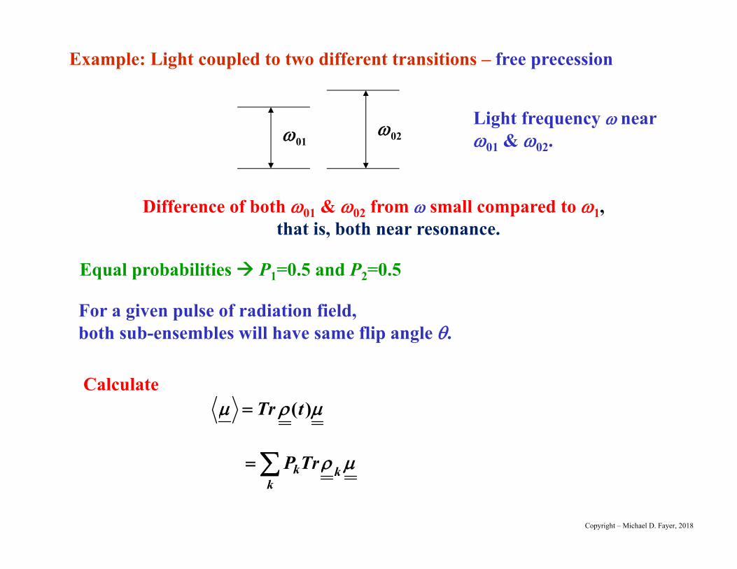
Example: Light coupled to two different transitions – free precession

01 02

Difference of both 01 & 02 from small compared to 1,that is, both near resonance.

Equal probabilities P1=0.5 and P2=0.5

( )Tr t

k kk

P Tr

For a given pulse of radiation field, both sub-ensembles will have same flip angle .

Calculate

Light frequency near 01 & 02.


0sin sin( )t

Pure density matrix result for flip angle :

For 2 transitions - P1=0.5 and P2=0.5

01 021 sin sin( ) sin( )2

t t

01 02 01 021 1sin sin ( ) cos ( )2 2

t t

from trig.identities

Call: center frequency 0, shift from the center then, 01 = 0 + and 02 = 0 - ,with << 0

0sin sin( )cos( )t t Therefore,

Beat gives transition frequencies – FT-NMR

high freq. oscillation low freq. oscillation, beat


5 10 15 20

-2

-1

1

2

Equal amplitudes – 100% modulation, ω01 = 20.5; ω01 = 19.5


5 10 15 20

-1

-0.5

0.5

1

Amplitudes 2:1 – not 100% modulation , ω01 = 20.5; ω01 = 19.5


5 10 15 20

-1

-0.5

0.5

1

Amplitudes 9:1 – not 100% modulation , ω01 = 20.5; ω01 = 19.5


5 10 15 20

-2

-1

1

2

Equal amplitudes – 100% modulation, ω01 = 21; ω01 = 19


Free Induction Decay center freq0

h frequencyof particular molecule

Frequently, distribution is a Gaussian -

probability of finding a molecule at a particular frequency, Ph.

Identical molecules haverange of transition frequencies.Different solvent environments.Doppler shifts, etc.

Gaussian envelope

2 20( ) / 2

2

1( ) ( , )2

hh ht e t d

2 20( ) /2

2

1

2h

hP e

standard deviation

normalizationconstant

Then

pure density matrixprobability, PhCopyright – Michael D. Fayer, 2018

Radiation field at = 0 line center 1 >> – all transitions near resonance

Apply pulse with flip angle

Calculate , transition dipole expectation value.

2 20( ) / 2

2

sin sin( )2

hh he t d

Using result for single frequency h and flip angle

Following pulse, each sub-ensemble will undergo free precession at h

( )Tr t

2 20( ) / 2

2

1 ( , )2

hh he Tr t d


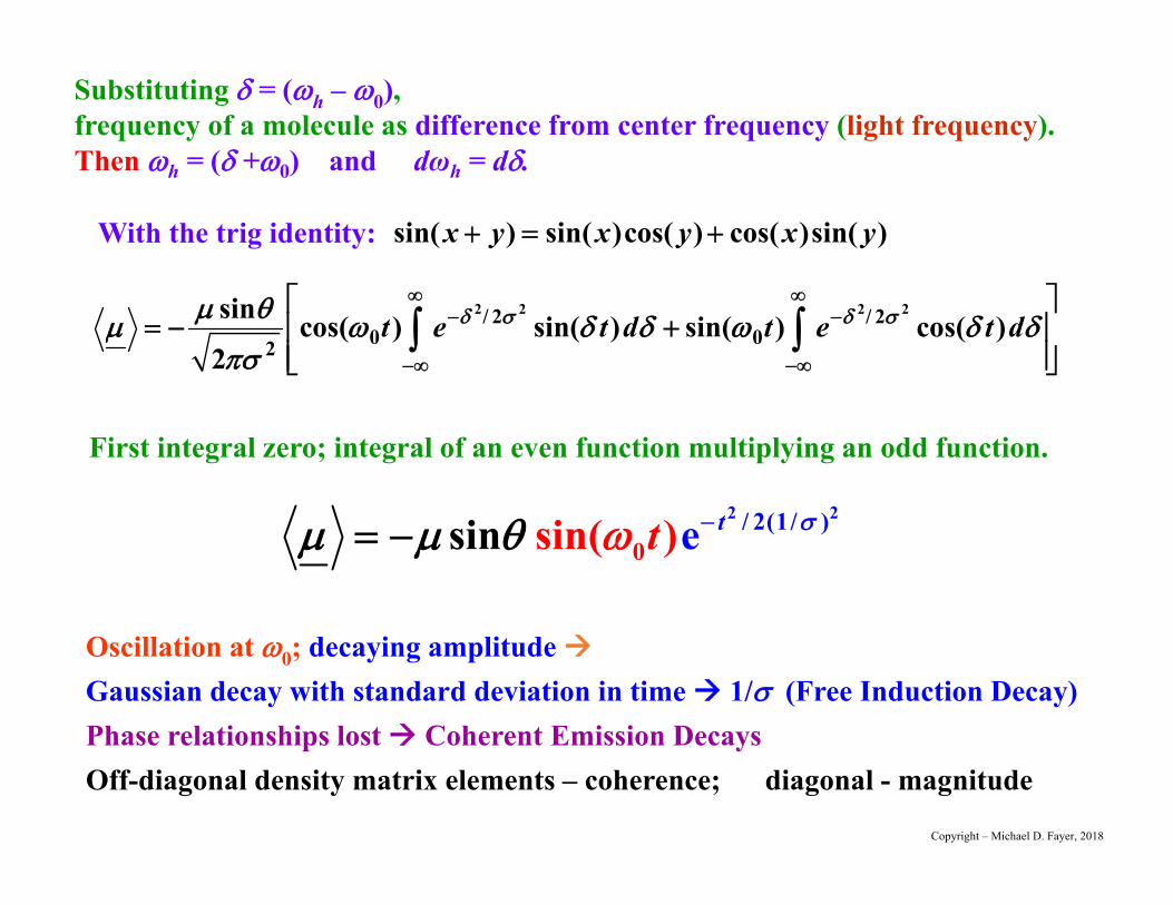
Substituting = (h – 0), frequency of a molecule as difference from center frequency (light frequency).Then h = ( +0) and dωh = d.

2 2/ 2( /0

1 )sin(in )es tt

Oscillation at 0; decaying amplitudeGaussian decay with standard deviation in time 1/ (Free Induction Decay)Phase relationships lost Coherent Emission DecaysOff-diagonal density matrix elements – coherence; diagonal - magnitude

2 2 2 2/ 2 / 20 02

sin cos( ) sin( ) sin( ) cos( )2

t e t d t e t d

First integral zero; integral of an even function multiplying an odd function.

sin( ) sin( )cos( ) cos( )sin( )x y x y x y With the trig identity:


flip angle light frequency free induction decay

0.5 1 1.5 2 2.5 3

0.2

0.4

0.6

0.8

1

Decay of oscillating macroscopic dipole.Free induction decay.

22

E

I E

Coherent emissionof light.

rotating frame at center freq., 0

higher frequencies

lower frequencies

t = 0 t = t'

2 2/ 2( /0

1 )sin(in )es tt


Chapter 14web.stanford.edu/group/fayer/lectures/R19/Chapter14R19.pdf · Density Matrix State of a...

Documents

Transcript of Chapter 14web.stanford.edu/group/fayer/lectures/R19/Chapter14R19.pdf · Density Matrix State of a...