Chapter 13Using a distributed SDP approach to solvesimulated protein molecular conformationproblems

Xingyuan Fang and Kim-Chuan Toh

Abstract This paper presents various enhancements to the DISCO algorithm (orig-inally introduced by Leung and Toh [18] for anchor-free graph realization inRd) forapplications to conformation of protein molecules inR3. In our enhanced DISCOalgorithm for simulated protein molecular conformation problems, we have incorpo-rated distance information derived from chemistry knowledge such as bond lengthsand angles to improve the robustness of the algorithm. We also designed heuris-tics to detect whether a subgroup is well localized and significantly improved therobustness of the stitching process. Tests are performed onmolecules taken fromthe Protein Data Bank. Given only 20% of the inter-atomic distances less than 6Athat are corrupted by high level of noises (to simulate noisydistance restraints gen-erated from nuclear magnetic resonance experiments), our improved algorithm isable to reliably and efficiently reconstruct the conformations of large molecules. Forinstance, given 20% of inter-atomic distances which are less than 6A and are cor-rupted with 20% multiplicative noise, a 5600-atom conformation problem is solvedin about 30 minutes with a root-mean-square-deviation (RMSD) of less than 1A.

13.1 Introduction

Determining protein structure is an important problem in biology. Majority of theprotein structures are obtained by X-ray crystallography.However, some proteinscould not be crystallized, and the information we have from its solution state is somepairwise atomic distance bounds (known as Nuclear Overhauser effect (NOE) dis-

Xingyuan FangDepartment of Operations Research and Financial Engineering, Princeton University, New Jersey,e-mail: xingyuan@princeton.edu

Kim-Chuan TohDepartment of Mathematics, National University of Singapore, Singapore-MIT Alliance, Singa-pore, e-mail: mattohkc@nus.edu.sg

253

254 Fang and Toh

tance restraints) estimated from nuclear magnetic resonance (NMR) spectroscopyexperiments. From late 1970s, distance geometry algorithms have become increas-ingly used in the interpretation of experimental data on macro molecular confor-mation. Generally, we use these algorithms to determine theCartesian coordinatesof the atoms of a molecule which are consistent with a predetermined set of in-tramolecular distance constraints. Those constraints could come from experimentaldata and known chemistry knowledge such as bond lengths and angles. In 1984, thestructure of the first protein determined in its native solution state from NMR datawas computed by the algorithm DISGEO [15].

The mathematical setting of the molecular conformation problem is as follows.We wish to determine the coordinates ofn atomsxxxi ∈ R3, i = 1, . . . ,n. The infor-mation that is available consists of measured distances or distance bounds for someof the pairwise distances||xxxi − xxx j || with (i, j) ∈ N , whereN is the set of indexpairs(i, j) for which inter-atomic distance information is available.Note that in ourconvention, we only consider the pair(i, j) with i < j. The molecular conformationproblem is an instance of the graph realization problem where the atoms are thevertices of the graph, and the pairs(i, j) ∈N are the edges with the weight of edge(i, j) specified by the given distance datadi j . In a p-dimensional graph realizationproblem, one is interested in determining points inRp such that||xxxi−xxx j || ≈ di j forall (i, j) ∈N .

The molecular conformation problem is closely related to thesensor network lo-calization problem, but much more challenging. In the sensor network localizationproblem, there are two classes of objects: anchors (whose locations are known a pri-ori) and sensors (whose locations are unknown and to be determined). In practice,the anchors and sensors are able to communicate with one another if they are not toofar apart (say within a certain cut-off range), to obtain an estimate of the distancefor each communicable pair. For the molecular conformationproblem, there are noanchors. And more importantly, not all pairs of atoms withinthe cut-off range havedistance estimates. In this paper, we will use the term “conformation”, “localiza-tion”, and “realization” interchangeably.

Recently, semidefinite programming (SDP) relaxation techniques have been ap-plied to the sensor network localization problem [3]. Whilethis approach was suc-cessful for moderate-size problems with the number of sensors in the order of a fewhundreds, it was unable to solve problems with a large numberof sensors, due tocomputational limitations in SDP algorithms for solving large scale problems. Tolocalize larger networks, a distributed SDP-based algorithm for sensor network lo-calization was proposed in [6]. The critical assumption required for the algorithmin [6] to work well is that there exist anchors distributed uniformly throughout thephysical space. As a result, the algorithm cannot be appliedto the molecular con-formation problem, since the assumption of uniformly distributed anchors does nothold in the case of molecular conformation.

In [4], a distributed SDP-based algorithm (called DAFGL) was proposed andtested for the molecular conformation problem. The performance of the DAFGLalgorithm is satisfactory when given 50% of pairwise distances less than 6A apartthat are corrupted by 5% multiplicative noise. More recently, Leung and Toh [18]

13 Using SDP approach for molecular conformation problems 255

proposed a new distributed approach, the DISCO (for DIStributed COnformation)algorithm, with a view towards applications in molecular conformation. The DISCOalgorithm was demonstrated to be efficient and robust in solving simulated molecu-lar conformation problems when given only 30% of the pairwise distances less than6A which are corrupted by 20% multiplicative noise. However,DISCO frequentlyfails to give good results when given only 20% pairwise distances less than 6A apart.

In this paper, we describe the DISCO algorithm and the enhancements we madeto make the algorithm work for the protein molecular conformation problem un-der the highly sparse distance data regime of using only 20% pairwise distancesless than 6A that are corrupted by high level of noise. We should mentionthatin this work, real NOE distance data from NMR experiments arenot considered,although that is our future goal. Instead, the distance datawe considered are sim-ulated from known protein conformations in order to validate the results obtainedby DISCO by comparing the reconstructed conformations to the original ones. Theprotein molecules we used in our experiments are downloadedfrom the ProteinData Bank (PDB). In our experiments, we discard all the hydrogen atoms in themolecules. The input distances (all in the unit ofA= 10−10 meter) are given aslying in intervals[di j ,di j ] for (i, j) ∈ N . HereN denotes the set of index pairs(i, j) for which inter-atomic distance bounds are available. In our simulated proteinmolecular conformation problem, we consider two types of distance bounds. Thefirst type of bounds come from known chemistry information such as bond lengthsand angles, and the interval is given in the form:

di j = (1− ε)di j , di j = (1+ ε)di j ∀ (i, j) ∈Nc (13.1)

whereε ∈ (0,0.1) is a parameter which can be chosen appropriately to reflect ourconfidence on the given distancedi j derived from the chemistry information of themolecule. The index setNc is used to denote the index pairs(i, j) for which distancebounds based on chemistry information are given. The secondtype of bounds aredesigned to simulate NOE restraints, and they are given as follows:

di j = max(

2.0,(1−σ |zi j |)di j

), di j = (1+ σ |zi j |)di j (i, j) ∈Ns, (13.2)

wheredi j is the true distance between atomsi and j, zi j ,zi j are independent randomvariables such that|zi j |, |zi j | have unit mean value. The parameterσ is the noisefactor which we typically set to 20%. The number 2.0 in the expression fordi j is aconservative lower bound on the shortest distance between two non-bonded (non-hydrogen) atoms. The index setNs is used to denote the index pairs(i, j) for whichthe simulated distance bounds are given. Note that the overall index setN is thedisjoint union ofNc andNs.

The main enhancements we made are as follows. First, we have included somedistances derived from basic chemistry information such asbond lengths and bondangles into the distance data used in the conformation. We relied on the papers [17]and [1] for those basic chemistry information. To automatically derive those chem-istry information for a protein molecule given its amino acids sequence, we find it

256 Fang and Toh

convenient to design a structure array data structure to code the information pertain-ing to each atom in the molecule. Second, we also designed effective heuristics todetect whether a subgroup of atoms is well localized, as wellas substantially im-proved the robustness of the stitching process in the DISCO algorithm. We demon-strate that our enhanced DISCO algorithm is efficient and robust, and it works wellunder the highly sparse distance data regime we have targeted. Compared to theoriginal DISCO algorithm, the RMSD errors of some reconstructed molecules havebeen significantly improved when given only 20% of pairwise distances (corruptedby 20% multiplicative noise) less than 6A. For example, the average RMSD of thereconstructed conformations for the molecule1RGS is reduced from 4.5A to 1.3Aover 10 random instances. We should mention that the 20% distances less than 6Aused to simulate NOE restraints is randomly selected from the set of all distancesless than 6A excluding those derived from chemistry knowledge.

As non-random test problems for evaluating sensor network localization algo-rithms are of interest to the sensor network community, we plan to make the distancedata we have generated in this paper publicly available at the following web-site:

http://www.math.nus.edu.sg/∼mattohkc/disco.html

The paper is organized as follows. Section 2 describes some existing molecularconformation algorithms; Section 3 details the mathematical models for molecularconformation based on SDP; Section 4 explains the design of DISCO and describesthe enhancements we made; Section 5 describes the chemistryinformation we haveincorporated into our simulated protein molecular conformation problems; Section6 contains the experimental setup and numerical results; Section 7 gives the conclu-sion.

In this paper, we adopt the following notational conventions. Lower case letters,such asn, are used to represent scalars. Lower case letters in bold font, such ass,are used to represent vectors. Upper case letters, such asX, are used to representmatrices. Upper case letters in calligraphic font, such asD , are used to representsets. Cell arrays will be prefixed by a letter “c”, such ascAest. Cell arrays will beindexed by curly braces{}.

13.2 Related Work

Due to its great importance, there are quite a number of existing algorithms to tacklethe molecular conformation problem. We discuss selected works in this section.Here we do not attempt to give a detailed survey of the existing work on the distancegeometry approach for solving the molecular conformation problem. Our intentionis only to highlight the most relevant work for which the experimental settings usedbear the closest similarity with ours. For the existing algorithms which we mentionin this section, we pay attention to each algorithm by the following aspects: themathematics, its input data, and the results it is able to provide. In particular, wemake a note of the largest molecule which each algorithm was able to solve and its

13 Using SDP approach for molecular conformation problems 257

error (mostly measured by RMSD) in the tests done by the authors. This informationis summarized in Table 13.1.

Before we begin, we note that from the theory of distance geometry [25, 26, 27],there is a natural correspondence between inner product matrices and Euclideandistance matrices. Thus it is quite common to solve the molecular conformationproblem by working with an inner product matrix. If we denotethe atom coordi-nates by column vectorsxxxi , and letX = [xxx1 . . .xxxn], then the inner product matrixis given byY = XTX. If we have a computedY, then we can recover the approxi-mate coordinatesX by taking the best rank-3 approximation based on the eigenvaluedecomposition ofY.

The earliest distance geometry based algorithm for molecular conformation isthe EMBED algorithm [14] developed by Havel, Kuntz and Crippen in 1983. Theinput data of EMBED consists of lower and upper bounds on someof the pairwisedistances. EMBED uses the triangle and tetrangle inequalities to compute distancebounds for all pairs of points, followed by choosing random numbers within thebounds to form an estimated distance matrixD (one should note that the triangleand tetrangle bounds are generally too weak to provide good estimates on the dis-tances). It checks whetherD is close to a valid rank-3 Euclidean distance matrixby considering the three largest eigenvalues (in magnitude) of Y, the inner productmatrix corresponding toD. In the fortunate case where the three eigenvalues arepositive and are much larger than the rest, this would indicate that the estimated dis-tance matrixD is close to a true distance matrix, and the coordinates obtained fromthe inner product matrix are likely to be acceptable. In the unfortunate case whereat least one of the three eigenvalues is negative, the estimated distance matrixD isfar from a valid distance matrix. In this case, EMBED repeatsthe step of choos-ing an estimated distance matrix until it obtains one that isclose to a valid distancematrix. As a postprocessing step, the coordinates are improved by applying localoptimization methods.

Subsequently, Havel and Wuthrich developed the DISGEO package [15] to im-prove the performance of EMBED. As the EMBED algorithm is unable to computea conformation of the whole protein structure, due to the high dimensionality ofthe problem, DISGEO uses two passes of EMBED to overcome the problem. Inthe first pass, coordinates are computed for a subset of atomssubject to constraintsinherited from the whole structure. In this step, EMBED usesdata not only fromexperiments, but also from chemistry knowledge, includingbond lengths, bond an-gles, hybridization theory, and so on. This step forms a ”skeleton” for the structure.The second pass of EMBED then computes coordinates for the remaining atoms,building upon the skeleton computed in the first pass. The authors tested the perfor-mance of DISGEO on theBPTI protein, which has 454 atoms. The input consists ofdistance (3290) and chirality (450) constraints needed to fix the covalent structure,and bounds (508) for distances between hydrogen atoms in different amino acidresidues that are less than 4A apart, to simulate the distance constraints availablefrom a nuclear Overhauser effect spectroscopy experiment.Using a pseudostructure

258F

angand

Toh

Algorithm(s) Largest molecule(No. ofatoms)

Inputs Output

EMBED (83),DISGEO (84),DG-II (91),APA (99)

454 All distance and chirality constraints needed to fix the co-valent structure are given exactly. Some or all of the dis-tances between hydrogen atoms less than 4A apart and indifferent amino acid residues given as bounds.

RMSD 2.08A

DGSOL (99) 200 All distances between atoms in successive residues givenas lying in[0.84di j ,1.16di j ].

RMSD 0.7A

GNOMAD (01) 1870 All distances between atoms that are covalently bondedgiven exactly; all distances between atoms that share co-valent bonds with the same atom given exactly; additionaldistances given exactly, so that 30% of the distances lessthan 6A are given; physically inviolable minimum separa-tion distance constraints given as lower bounds.

RMSD 2–3A(*)

MDS (02) 700 All distances less than 7A were given as lying in[di j −0.01,di j +0.01].

violations< 0.01A

StrainMin (06) 5147 All distances less than 6A are given exactly, a representa-tive lower bound of 2.5A is given for other pairs of atoms.

violations< 0.1A

ABBIE (95) 1849 All distances between atoms in the same aminoacid givenexactly. All distances between pairs of hydrogen atoms lessthan 3.5A apart, given exactly.

Exact

Geometric build-up (07) 4200 All distances between atoms less than 5A apart given ex-actly.

Exact

DAFGL (07) 5681 70% of the distances less than 6A were given as lyingin [di j ,di j ], where di j = (1− 0.05|zi j |)+di j ,di j = (1 +

0.05|zi j |)di j , andzi j ,zi j are standard normal random vari-ables with zero mean and unit variance.

RMSD 3.16A

Table13.1

Asum

mary

ofproteinconform

ationalgorithm

s.(*)T

heR

MS

Do

f1.07 Areported

byG

NO

MA

Dm

aybe

incorrect,and

thetrue

valueshould

beabout

2–3A

sincethe

number

reportedin

Figure

11of[29

]doesnotagree

with

thatappearsin

Figure8.

13 Using SDP approach for molecular conformation problems 259

representation, they were able to solve for 666 geometric points1. Havel’s DG-IIpackage [13], published in 1991, improves upon DISGEO by producing from thesame input as DISGEO five structures having an average RMSD of1.76A from thecrystal structure.

The work in this paper is a continuation of the DISCO algorithm developed in2009 [18]. DISCO differs from the previous methods in that itapplies SDP relax-ation methods to obtain the inner product matrix. In order tosolve larger problems,it employs a divide-and-conquer approach for which each basis group is solved us-ing SDP, and the overlapping groups are used to align the local solutions to form aglobal solution. Tests were performed on 14 molecules with number of atoms rang-ing from 400 to 5600. The input data consists of 30% of the distances below 6A,given as lying in intervals[di j ,di j ] which are generated from the true distancesdi j

with 20% multiplicative noises added. Given such input, DISCO is able to producea conformation for most molecules with an RMSD of 2–3A.

Distributed algorithms (based on successive decomposition) similar to thosein [4] were proposed for fast manifold learning in [30, 31]. In addition, those pa-pers also considered recursive decomposition. The manifold learning problem is toseek a low-dimensional embedding of a manifold in a high dimensional Euclideanspace by modeling it as a graph-realization problem. The resulting problem has sim-ilar characteristics as the molecular conformation problem (which is an anchor-freegraph realization problem) we consider in this paper, but there are some importantdifferences which we should highlight. For the manifold learning problem, exactpairwise distances between any pairs of vertices (atoms in our case) are available,but for the molecular conformation problem, only a very sparse subset of pairwisedistances are assumed to be given and are only known within a given range. Such adifference implies that for the former problem, any local patch will have a “unique”embedding (up to rigid motion and certain approximation errors) computable via aneigenvalue decomposition, and the strategy to decompose the graph into sub-graphsis fairly straightforward. In contrast, for the latter problem, given the sparsity of thegraph and the noise in the distances data, the embedding problem itself requires anew method, not to mention that sophisticated decomposition strategies also needto be devised.

The GNOMAD algorithm [29] by Williams, Dugan and Altman is a gradientdescent based algorithm which attempts to satisfy the inputdistance constraints aswell as minimum separation distance (MSD) constraints. Their algorithm appliesto the situation when we are given sparse but exact distances. The knowledge ofMSD constraints is useful in limiting the search space, but if they are not appliedintelligently, they may trap the algorithm at an unsatisfactory local minimum. Sinceit is difficult to optimize all the atom positions simultaneously because of the highdimensionality of the problem, GNOMAD updates the positions of the atoms oneatom at a time. The authors tested GNOMAD on the protein molecule 1TIM, which

1 In NMR experiments, certain protons may not be stereospecifically assigned. For such pairs ofprotons, the upper bounds are modified via the creation of “pseudoatoms”, as is the standard prac-tice in NOE experiments. given 3798 distance and 450 chirality constraints, with three computedstructures having an average RMSD of 2.08A from the known crystal structure.

260 Fang and Toh

has 1870 atoms. Given all the covalent distances and distances between atoms thatshare covalent bonds to the same atom, as well as 30% of pairwise distances lessthan 6A, they were able to compute a conformation with an RMSD of 2–3A2. Theexperimental setting we considered in this paper is similarto that given in [29], butin the highly challenging regime of having very sparse and noisy distances. Also thealgorithm we designed is completely different from GNOMAD.Our algorithm’sinput includes all the covalent distances and distances between atoms that sharecovalent bonds with the same atom. We also add 20% of pairwisedistances lessthan 6A (which are corrupted by high level of noise) to simulate distances derivedfrom an NMR experiment.

In this brief discussion on related work, we have not touchedon approaches basedon global optimization and discrete optimization methods.For example, in [19], theauthors developed a branch-and-prune method. We refer the reader to [19], [18] and[29] for more detailed review of various distance geometry based methods includingthose in [16], [9], [11], [21], proposed for the molecular conformation problem.

13.3 Optimization models for the molecular conformationproblem

We begin this section with the optimization models we consider for the molecu-lar conformation problem. Then we introduce the semidefinite programming (SDP)relaxations for these models, and describe the gradient descent method we adoptfor improving the positions of the atoms by using the SDP solution as the startingpoint. Finally, we present the alignment problem for stitching (sometimes we willalso use the words “merging” and “combining”) two groups of atoms together usingthe overlapping atoms in the groups.

13.3.1 Semidefinite programming models

In the “measured distances” model, we have measured distancesdi j for certain pairsof atoms, i.e.,

di j ≈ ||xxxi−xxx j || (i, j) ∈N . (13.3)

In this model, the unknown positions{xxxi}ni=1 represents the best fit to the measureddistances, obtained by solving the following nonconvex minimization problem:

min

{

∑(i, j)∈N

∣∣||xxxi−xxx j ||2− (di j )2∣∣}

. (13.4)

2 The RMSD of 1.07A reported in Figure 11 in [29] is inconsistent with that appearing in Figure 8.It seems that the correct RMSD should be about 2–3A.

13 Using SDP approach for molecular conformation problems 261

For convenience, we denote the measured inter-atomic distance matrix byD. In the“distance bounds” model, we have lower and upper bounds on the distances betweencertain pairs of atoms, i.e.,

di j ≤ ||xxxi−xxx j || ≤ di j (i, j) ∈N . (13.5)

In this model, the unknown positions{xxxi}ni=1 represent any feasible solutionX =[xxx1, . . . ,xxxn] satisfying the bound constraints. We denote the lower and upper bounddistance matrices byD, D. Note that for the “distance bounds” model, we can natu-rally convert it to the “measured distance” model by takingdi j = (di j +di j )/2.

In order to proceed to the SDP relaxation of the problem, we consider the fol-lowing matrix

Y := XTX, whereX = [xxx1 . . .xxxn]. (13.6)

Let {eeei}ni=1 be set of standard unit vectors inRn. By denotingeeei j = eeei−eeej , we notethat

||xxxi−xxx j ||2 = eeeTi jYeeei j .

We can therefore conveniently express the constraints in (13.3) and (13.5) respec-tively as

(di j )2 ≈ eeeT

i jYeeei j (i, j) ∈N

(di j )2 ≤ eeeT

i jYeeei j ≤ (di j )2 (i, j) ∈N .

The SDP relaxation then consists in relaxing the constraint“Y = XTX” in (13.6) intothe constraint “Y � 0”, where the notation means that then×n symmetric matrixYis positive semidefinite.

The SDP relaxation of the measured distances model (13.4) isgiven by

min

{

∑(i, j)∈N

∣∣eeeTi jYeeei j − (di j )

2∣∣ | Y � 0

}. (13.7)

Similarly we can express the SDP relaxation of the distance bounds model (13.5) asfinding an element in the following set:

{Y | (di j )

2 ≤ eeeTi jYeeei j ≤ (di j )

2 ∀ (i, j) ∈N , Y � 0}

. (13.8)

Once we have obtained a matrixY by solving either (13.7) or (13.8), we can estimatethe atom positionsX = [xxx1 . . .xxxn] by settingX to be the best rank-3 approximationof Y.

In [4], it has been shown that if the distance data is exact andthe conformationproblem is uniquely localizable, then the SDP relaxation (13.7) is able to producethe exact atom coordinates up to a rigid motion. We refer the reader to [4] for thedefinition of “uniquely localizable”. Intuitively, it means that there is only one con-figuration inR3 (up to a rigid motion) that satisfies all the distance constraints. The

262 Fang and Toh

result (which is a variant of the result established by So andYe [22] for graph re-alization with anchors) gives a strong indication that the SDP relaxation techniqueis a powerful relaxation. We can therefore hope that applying SDP relaxation toproblems with sparse and noisy distance data will be effective.

We now discuss what typically would happen when the distancedata is sparseand/or noisy, so that there is no unique realization. In sucha situation, it is notpossible to recover the true coordinates. Furthermore, thesolutionY of the SDP(13.7) or (13.8) will generally have rank greater than 3, as we shall explain next.Suppose we have points in the plane, and certain pairs of points are constrained sothat the distance between them is fixed. If the distances are perturbed slightly, thensome of the points may be forced out of the plane in order to satisfy the distanceconstraints. Therefore, for noisy distance data,Y will tend to have a rank higher than3. Another reason forY to have a higher rank is that, if there are multiple optimalsolutions in an SDP problem, interior-point methods used bymany SDP solverswould converge to a solution with maximal rank [12].

This situation leads to potential issues. IfY has a rank higher than 3, then the bestrank-3 approximation ofY is unlikely to give accurate positions for the atoms. Toameliorate this difficulty, we add the following regularization term into the objectivefunction, i.e.,

−γ〈I ,Y〉 (13.9)

whereγ is a positive regularization parameter. The motivation forintroducing thisterm is to spread the atoms further apart so as to induce them to lie in a lower-dimensional space. Indeed, under the condition that 0= ∑n

i=1xxxi = Xeee, whereeee∈Rn

is the vector of all ones, we can easily show that∑ni=1 ∑n

j=1 ||xxxi−xxx j ||2 = 〈I ,Y〉/(2n)

by using the definition thatY = XTX. We refer interested readers to [3] for detailson the derivation of the regularization term. Thus, for the measured distances model,the regularized SDP model for (13.7) becomes

min

{

∑(i, j)∈N

|eeeTi jYeeei j − (di j )

2|− γ〈I ,Y〉 | eeeTYeee= 0, Y � 0

}(13.10)

and the one related to the distance bounds model (13.8) becomes

min{−〈I ,Y〉 | (di j )

2 ≤ eeeTi jYeeei j ≤ (di j )

2 ∀ (i, j) ∈N , eeeTYeee= 0, Y � 0}

.(13.11)

Note that we have added the constraint “eeeTYeee = 0” to reflect the requirement forwhich the center of massXeee is fixed to the origin.

We should emphasize that as observed in [3], the inclusion ofthe regularizationterm in the SDP model can greatly improve the quality of the conformation solu-tion X generated by the SDP model together with a subsequent gradient descentrefinement. However, the choice of the regularization parameterγ is crucial. In ourimplementation of the enhanced DISCO algorithm, we adaptively adjust the valueof γ based on the following separation ratio:

13 Using SDP approach for molecular conformation problems 263

sep ratio=1|N | ∑

(i, j)∈N

si j , wheresi j =||xxxi−xxx j ||

di j. (13.12)

Observe that, if the solutionX generated by the SDP model is the correct conforma-tion anddi j is the exact distance between atomsi and j for all (i, j) ∈N , then wemust havesep ratio=1. Of course, for noisy distances,sep ratio would not beexactly 1, but we expect the value to be close to 1 if the computed conformationis not too different from the true one. In fact, from our extensive numerical exper-iments, we find that the value ofsep ratio should generally lie in the interval[0.85,1.1] in order for the conformation solution (generated from the SDP model)to have a reasonably good quality (measured in terms of the RMSD with respect tothe true conformation). Based on such a criterion, we increaseγ if sep ratio istoo small, and decrease it ifsep ratio is too big. If after 5 trials, we cannot getsep ratio to lie in the required interval, we declare that the underlying conforma-tion problem{di j |(i, j) ∈N } is not localizable, and flag it as “bad”.

Note that, in a distributed algorithm like DISCO, it is very important for us todesign a reasonably good heuristic to detect whether a configuration is bad. Thisis because a bad configuration should not be stitched to a good(well localized)configuration for otherwise it will destroy the good one after the two configurationsare aligned and stitched. A bad configuration should be separately handled after themajority of the atoms in the molecule have been localized.

13.3.2 Coordinate refinement via gradient descent

If we are given measured pairwise distancesdi j , then the atoms’ coordinates can alsobe computed as the minimizer of the following nonconvex minimization problem:

min f (X) := ∑(i, j)∈N

(||xxxi−xxx j ||− di j

)2 −βn

∑i=1

n

∑j=1||xxxi−xxx j ||2. (13.13)

Note that the above objective function is different from that of (13.4) because wewant it to be differentiable. Observe that as in our SDP model, we have added aregularization term (with positive parameterβ ) in the objective function in (13.13).Similarly, if we are given boundsdi j ,di j for pairwise distances, then the configura-tion can be computed as the solution of the following problem:

min ∑(i, j)∈N

(||xxxi−xxx j ||−di j

)2−+

(||xxxi−xxx j ||−di j

)2+−β

n

∑i=1

n

∑j=1

||xxxi−xxx j ||2.

(13.14)We can solve (13.13) or (13.14) by applying local optimization methods. For sim-plicity and computational efficiency, we choose to use a gradient descent methodwith backtracking line search. The algorithmic framework of this method is ratherstraightforward, so we shall omit the details. It is a simpleexercise in calculus to

264 Fang and Toh

find the gradient off with respect to the coordinate vectorxxxi . However, we shouldemphasize that, to compute the gradient efficiently, the computation must be de-signed appropriately. In our implementation, we find it convenient to construct then×|N | sparse node-arc incidence matrixE for which the(i, j)-th column containsonly two non-zero entries with 1 and−1 at row i and j, respectively. WithE, wehave thatXE = [xxxi−xxx j | (i, j) ∈N ]. Thus to calculate[||xxxi−xxx j || | (i, j) ∈N ], onejust needs to take the norm of the columns ofXE.

The problems (13.13) and (13.14) are highly nonconvex problems with many lo-cal minimizers. Thus, if the initial iterateX0 is not close to a good local minimizer,then it is extremely unlikely that the resultingX obtained from a local optimizationmethod will be a good solution. In our case, however, when we setX0 to be the con-formation produced from solving the SDP relaxation, local optimization methodsare often able to produce anX which improves upon the solutionX0 obtained fromthe SDP relaxation.

We should note that, while adding the regularization term in(13.13) and (13.14)(with a suitably chosen parameterβ ) would generally lead to a more accurate con-formation solutionX, it can sometimes (though rarely happen) give a much worsesolution if the parameterβ is chosen to be too large. In our implementation of theenhanced DISCO algorithm, we guard against such a bad case byexamining thefollowing expansion ratio:

expansion ratio= max{||xxxi ||/||xxx0i || | i = 1, . . . ,n},

where the columns ofX0 and X are translated to have their respective center ofmass at 0. If the expansion ratio is larger than 3, we declare that the solutionX isworse thanX0, and we discard the solutionX from the refinement process. In ourmore sophisticated implementation, we would perform another pass of the gradientdescent refinement by deleting the potentially “bad” atoms and their correspondingdistances from the optimization model while also reducing the parameterβ . Bydoing so, one hopes that the coordinates of the remaining atoms can be improved.

13.3.3 Alignment of configurations

A molecular configuration has translational, rotational, and reflective freedom. Nev-ertheless, we need to be able to compare two configurations todetermine how simi-lar they are. In order to do so, it is necessary to align them ina common coordinatesystem. Given{xxxi}ni=1 and{yyyi}ni=1, we can define the “best” alignment as the affinetransformationT that minimizes the following problem:

minccc∈R3,Q∈R3×3

{n

∑i=1

||T(xxxi)−yyyi ||2 | T(xxxi) = ccc+Q(xxxi) ∀ i, Q is orthogonal

}.(13.15)

13 Using SDP approach for molecular conformation problems 265

The functional form ofT restricts it to be a combination of translation, rotationand reflection. In the special case when the columns ofX = [xxx1, . . . ,xxxn] andY =[yyy1, . . . ,yyyn] are centered at the origin, (13.15) reduces to the followingorthogonalprocrustes problem

minQ∈R3×3

{||QX−Y||F | Q is orthogonal} .

It is well known that the optimalQ can be computed from the singular value decom-position ofXYT .

13.4 The basic ideas of the DISCO algorithm

Here we present the basic ideas of the DISCO algorithm (for DIStributed COnfor-mation). For the detail algorithm, we refer the reader to [18].

Before having DISCO, we could solve the molecular conformation problem byusing the SDP relaxation technique and gradient descent refinement if the moleculewas not too big (say the number of atoms was below 500). The aimof DISCO is tosolve large-scale problems.

A natural idea to solve a large conformation problem is to employ a divide-and-conquer approach, which applies the following general framework. If the numberof atoms is not too large, then solve the conformation problem via SDP, and applygradient descent refinement to improve the coordinates; otherwise break the atomsinto two subgroups, solve each subgroup recursively, and align and stitch them backtogether subsequently, again postprocessing the coordinates by applying gradientdescent refinement after each stitching step.

We find that the use of the divide-and-conquer approach not only allow us tosolve larger problem. It also allows us to design a more robust algorithm. For ex-ample, the repeated use of gradient descent refinement aftereach stitching step hascertainly helped DISCO to become much more successful in producing accurateconformations. As a by-product of the divide-and-conquer process, we find that cer-tain information collected during the SDP localization andstitching steps in DISCOcan be used to help us to design a more robust algorithm.

Next we describe how DISCO (a) recursively divides a molecule into two sub-groups of atoms; and (b) how to stitch (as well as how to decidewhether to stitch)two processed subgroups together. The idea DISCO uses to tackle the first issue is tominimize the number of edges between the two subgroups. The reason is that whena group is split into two disjoint subgroups, the edges (distances) between the twosubgroups are lost. In other words, some distance information is lost. Thus DISCOtries to minimize the information lost. For the second issue, DISCO’s strategy is forthe two subgroups to have overlapping atoms. If the overlapping atoms are accu-rately localized in the two subgroups, then they can be aligned for the purpose ofstitching the two subgroups together. If not, it would not bea good idea to align andstitch them since a bad subgroup can destroy the good one whenthey are stitched

266 Fang and Toh

together. Therefore, DISCO designed a heuristic criterionfor determining whetherthe overlapping atoms are accurately localized. In order tohave a reliable alignmentbased on the overlapping atoms in the two subgroups, one of the most obvious crite-rion is that the RMSD of the coordinates of the overlapping atoms contained in thetwo subgroups must not be large, say less than 3A; otherwise, it gives a strong indi-cation that at least one of the two subgroups is not well localized. We have observedthat the RMSD of the overlapping atoms used in the stitching of two subgroups pro-vides valuable information on the quality of the larger stitched configuration. Thus,for each stitched configuration, we assign a quality index (q index) as follows:

q index= max

RMSD ofoverlappingatoms

,1|N ′| ∑

(i, j)∈N ′max

(s5i j ,s−5i j

)

(13.16)

wheresi j is defined as in (13.12),N ′ is the subset ofN involved in the stitchedconfiguration, but it excludes the large outlier values of more than 100 in max(s5

i j ,s−5i j ).

The power of 5 in (13.16) is chosen based on empirical experience. At the basislevel, the quality index is assigned based on the SDP solution Y obtained from(13.10) or (13.11) as follows:

q index=

(1|N ′| ∑

(i, j)∈N ′max

(s5i j ,s−5i j

))1/2

wheresi j is calculated based on the best rank-3 approximationX = [xxx1, . . . ,xxxn′ ] ofthe SDP solutionY. If a basis configuration is already declared as “bad”, we setitsq index to be∞. Note that in the case of sensor network localization with exactdistance data, it has been demonstrated in [5] that the quantity Yii − ||xxxi ||2 givesan error measure of the estimated position for theith point. Unfortunately, whenthe distance data is highly noisy, that error measure has no obvious correlation tothe underlying accuracy of the computed positionxxxi . Thus we cannot use{Yii −||xxxi ||2 | i = 1, . . . ,n} to assign a value forq index.

To summarize, suppose we have two subgroups with quality indices,q index1

andq index2, and that they have sufficient number (which we set a threshold of 8atoms) of overlapping atoms with a dense underlying subgraph, roughly speaking,we will stitch the two subgroups together only if max{q index1,q index2} < 3,and that the RMSD of the overlapping atoms in the two subgroups is less than 3A.

Despite our rather effective heuristics to detect whether asubgroup is well local-ized, and to decide whether two subgroups should be stitched, we should point outthat DISCO may still fail to work for some cases (we refer the reader to [18] fordetails). Thus, it is necessary to invest more effort to partition a group of atoms intolocalizable subgroups, and improve the heuristics for detecting badly localized sub-groups. In our work, after incorporating chemistry information to the input distancedata, we observe that it becomes slightly easier to partition a group of atoms intotwo localizable subgroups.

13 Using SDP approach for molecular conformation problems 267

The pseudocode of the DISCO algorithm is presented in Algorithm 7. We illus-trate how the DISCO algorithm solves a small molecule in Figure 13.1.

Algorithm 7 The DISCO algorithm1: procedure DISCO(L,U)2: if number of atoms< basis sizethen3: [cAest,cI]← DISCOBASIS(L,U)4: else5: [cAest,cI]← DISCORECURSIVE(L,U)6: end if7: [cAest,cI]← DISCOPATCH(L,U)8: return cAest,cI9: end procedure

1: procedure DISCOBASIS(L,U)2: cI ← L IKELY LOCALIZABLE COMPONENTS(L,U)3: for i = 1, . . . ,LENGTH(cI) do4: cAest{i} ← SDPLOCALIZE(cI{i},L,U)5: cAest{i} ← REFINE(cAest{i},cI{i},L,U)6: end for7: return cAest,cI8: end procedure

1: procedure DISCORECURSIVE(L,U)2: [L1,U1,L2,U2]← PARTITION(L,U)3: [cAest1,cI1]← DISCO(L1,U1)4: [cAest2,cI2]← DISCO(L2,U2)5: cAest← [cAest1,cAest2]6: cI ← [cI1,cI2]7: repeat8: [cAest,cI]← COMBINECHUNKS(cAest,cI)9: [cAest,cI]← REFINE(cAest,cI,L,U)

10: until no change11: return cAest,cI12: end procedure

13.5 Chemistry information

In this section, we describe the chemistry information we have added to the inputdistance data for DISCO.

268 Fang and Toh

Fig. 13.1 (top left and right) Since the number of atoms is too large (n = 402> basis size=300), we divide the atoms into two subgroups. (middle left and right) We solve the subgroupsindependently. (bottom left) The subgroups have overlapping atoms, which are colored in green.(bottom right) The overlapping atoms allow us to align the two subgroups to form a conformationof the molecule.

13 Using SDP approach for molecular conformation problems 269

13.5.1 Backbone distances

It well known that a protein molecule contains a backbone (which serves as themain “skeleton” of the molecule) from which the general shape of the molecule isdetermined; see Figure 13.2 for a schematic diagram of a backbone.

Fig. 13.2 A schematic diagram of a protein backbone, whereRk denotes the side chain of thekthamino acid.

The most commonly known distance information between atomsin a moleculeare bond lengths and bond angles. Given bond lengths and bondangles, we caneasily calculate the distance between two atoms which are bonded to the same atomby the cosine law. Our first attempt is to incorporate known distance informationfor atoms in the protein molecule into our simulated proteinstructure determinationproblem. Specifically, we incorporate the following known distances.

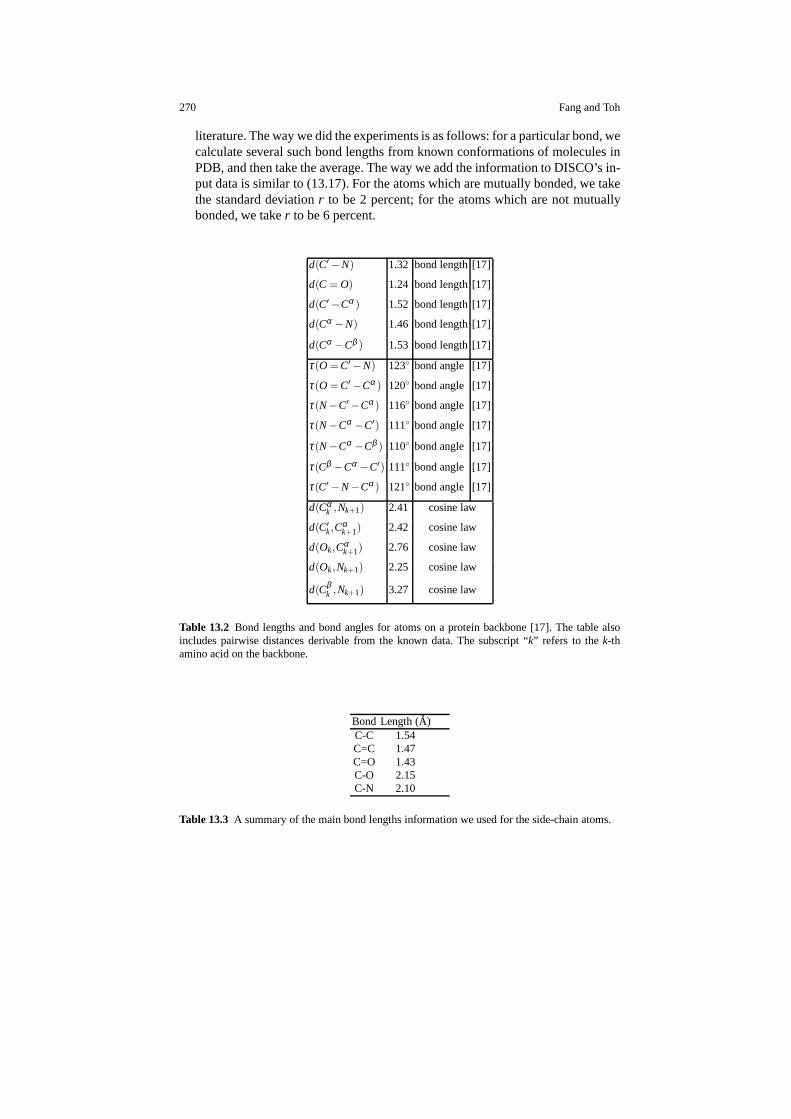
(a) Bond lengths of bonded pairs of atoms along the backbone,and distancesbetween non-bonded atom pairs along the backbone which are derivable basedon known bond lengths and bond angles by using the cosine law.The informationwe use comes mainly from the paper by R.Laskowski and D.Moss [17], and crosschecked with the data in [10]. The mean distances between various atom pairsalong the backbone are given in Table 13.5.1. Since the bond lengths and bondangles are not known perfectly, but within small standard deviations around somemean values, we add the distance information in the form of lower and upperbounds as follows:

di j = di j (1− r), di j = di j (1+ r), (13.17)

wheredi j is the mean distance, andr is the standard deviation. For the distancecoming from a bonded atom pair, we taker to be 1 percent; for a non-bondedpair, we taker to be 3 percent.(b) Bond lengths of bonded pairs of atoms in the side chains. The main informa-tion we use is from a standard organic chemistry textbook [20] and a paper byW. Cornell and P. Cieplak [7]. The values we use are shown in Table 13.3. Asthere are too many kinds of bonds, we do not show all of them in the table. Wealso conduct experiments to find some bond lengths which are not found in the

270 Fang and Toh

literature. The way we did the experiments is as follows: fora particular bond, wecalculate several such bond lengths from known conformations of molecules inPDB, and then take the average. The way we add the informationto DISCO’s in-put data is similar to (13.17). For the atoms which are mutually bonded, we takethe standard deviationr to be 2 percent; for the atoms which are not mutuallybonded, we taker to be 6 percent.

d(C′−N) 1.32 bond length[17]

d(C = O) 1.24 bond length[17]

d(C′−Cα ) 1.52 bond length[17]

d(Cα −N) 1.46 bond length[17]

d(Cα −Cβ ) 1.53 bond length[17]

τ(O = C′−N) 123◦ bond angle [17]

τ(O = C′−Cα ) 120◦ bond angle [17]

τ(N−C′−Cα ) 116◦ bond angle [17]

τ(N−Cα −C′) 111◦ bond angle [17]

τ(N−Cα −Cβ ) 110◦ bond angle [17]

τ(Cβ −Cα −C′) 111◦ bond angle [17]

τ(C′−N−Cα ) 121◦ bond angle [17]

d(Cαk ,Nk+1) 2.41 cosine law

d(C′k,Cαk+1) 2.42 cosine law

d(Ok,Cαk+1) 2.76 cosine law

d(Ok,Nk+1) 2.25 cosine law

d(Cβk ,Nk+1) 3.27 cosine law

Table 13.2 Bond lengths and bond angles for atoms on a protein backbone [17]. The table alsoincludes pairwise distances derivable from the known data.The subscript “k” refers to thek-thamino acid on the backbone.

Bond Length (A)C-C 1.54C=C 1.47C=O 1.43C-O 2.15C-N 2.10

Table 13.3 A summary of the main bond lengths information we used for theside-chain atoms.

13 Using SDP approach for molecular conformation problems 271

As mentioned in the Introduction, to automatically derive the chemistry informa-tion for a protein molecule given its amino acids sequence, we find it convenientto design a structure array data structure to code the information pertaining to eachatom in the molecule. As an example, for the 402-atom proteinmolecule1PTQ, weuse an 1×402 structure array (sayp) with fields’c’, ’a’, ’aa’, ’am’ to storethe information pertaining to the molecule. The first two elements ofp are shownbelow:

p(1).c=[5.7208,-2.5088,10.2270] ,

p(1).a=’N’, p(1).aa=’HIS’, p(1).am=’N’

p(2).c=[5.2388,-1.4878,9.2950],

p(2).a=’C’, p(2).aa=’HIS’, p(2).am=’CA’

Herep(1).c refers to the known coordinates of the first atom;p(1).a refers tothe type of atom;p(1).aa refers to the amino acid for which the first atom residesin; p(1).am refers to the atomic label of the first atom with respect to theaminoacid it resides in.

13.5.2 van der Waals radii

We have also tried to add more lower bounds to our input data based on van derWaals radii. The van der Waals radius of an atom is half the minimum separationdistance between two atoms (of the same type) which are not chemically related toeach other. By carrying out empirical study using proteins from PDB, we found thatvan der Waals radii provide a good lower bound for the pairwise distance of atomswhich are at least three bonds away in the molecule. Note thatatomic radii can alsobe used to generate lower bounds for pairwise distances. Butthe van der Waals radiigive better lower bounds as they are normally twice as large as atomic radii.

The van der Waals radii we used are from a standard inorganic textbook [2],which are given as follows: C (1.70A), N (1.55A), O (1.52A), S (1.80A).

However, after experimenting with additional lower boundsgenerated from vander Waals radii, we found that the results usually do not improve significantly. Inaddition, the time taken to solve the conformation problem becomes significantlylonger because of the large number of additional lower bounds we have to handle.

The reason for not getting better results after adding the van der Waals radiimight be as follow. For the input pairwise distances, thoughthey are not exact, theyare estimators of the true pairwise distances. But for van der Waals radii generatedlower bounds, they are generally too weak to give useful information on the pairwisedistances. Thus, adding van der Waals radii generated lowerbounds are not reallyuseful. Since it also increases the computational cost by doing so, we have decidednot to add van der Waals radii generated lower bounds into ouralgorithm.

272 Fang and Toh

13.6 Numerical Experiments

Here we explain the computational issues in the DISCO algorithm. In Section13.6.1, we present the experimental setup. In Section 13.6.2, we discuss the nu-merical results.

13.6.1 Experimental Setup

The source codes for our DISCO algorithm are written in MATLAB , and the SDPT3software package of Toh, Todd and Tutuncu [24, 28, 23] is used to solve the SDPproblems arising in the DISCOBASIS step of the algorithm.

We perform the numerical experiments on a dual-processor machine (3.2GHzIntel Core i5) with 4GB RAM, running MATLAB version 7.8 using only one pro-cessor.

We tested our algorithm using input distance data obtained from a set of 7molecules taken from the Protein Data Bank. The conformations of these moleculesare already known, so we can compare our computed conformations to the true con-formations.

For the input distance data, we have two types of distance bounds. The first typeof bounds come from chemistry information pertaining to themolecule and the sec-ond type of bounds are generated randomly to simulate NOE restraints. The sparsityof the simulated NOE distance bounds was modeled by choosingat random a pro-portion of all the short-range pairwise distances less thanthe cut-off range of 6A,subject to the condition that the distance graph is connected3. The cut-off range of6A was selected because NMR techniques are able to give us distance informationbetween some pairs of atoms only if they are less than approximately 6A apart. Wehave adopted this particular input data model because it is simple and fairly real-istic [29, 4]. In realistic molecular conformation problems, exact inter-atomic dis-tances are not given, but only lower and upper bounds on the inter-atomic distancesare known. Thus, after selecting a certain proportion of short-range inter-atomicdistances, we add noise to the distances to give us lower and upper bounds. In thispaper, we have experimented with a “normal” and a “uniform” noise model. Thenoise level is specified by a parameterσ , which indicates the expected value of thenoise. When we say we have a noise level of 20%, what that meansis thatσ = 0.2.In the normal noise model, the bounds are specified by

di j = max(

αi j ,(1−σ |zi j |)di j

), di j = (1+ σ |zi j |)di j ,

wherezi j ,zi j are independent normal random variables with zero mean and standard

deviation√

π/2. Consequently, the expected value of|zi j |, |zi j | is 1, and the variance

3 The interested reader may refer to the code for the details ofhow the selection is done.

13 Using SDP approach for molecular conformation problems 273

is π/2−1. The positive scalarαi j in di j is the minimum separation distance betweenatomsi and j, and we will discuss how it is chosen in the next paragraph.

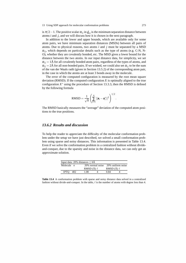
In addition to the lower and upper bounds, which are available only for someatom pairs, we have minimum separation distances (MSDs) between all pairs ofatoms. Due to physical reasons, two atomsi and j must be separated by a MSDαi j , which depends on particular details such as the type of atoms (e.g. C-N, N-O), whether they are covalently bonded, etc. The MSD gives a lower bound for thedistance between the two atoms. In our input distance data, for simplicity, we setαi j = 1A for all covalently bonded atom pairs, regardless of the types of atoms, andαi j = 2A for all non-bonded pairs. If we wished, we could also setαi j to be the sumof the van der Waals radii (given in Section 13.5.2) of the corresponding atom pair,in the case in which the atoms are at least 3 bonds away in the molecule.

The error of the computed configuration is measured by the root mean squaredeviation (RMSD). If the computed configurationX is optimally aligned to the trueconfigurationX∗ using the procedure of Section 13.3.3, then the RMSD is definedby the following formula

RMSD=1√n

(n

∑i=1

||xxxi−xxx∗i ||2)1/2

.

The RMSD basically measures the “average” deviation of the computed atom posi-tions to the true positions.

13.6.2 Results and discussion

To help the reader to appreciate the difficulty of the molecular conformation prob-lem under the setup we have just described, we solved a small conformation prob-lem using sparse and noisy distances. This information is presented in Table 13.4.Even if we solve the conformation problem in a centralized fashion without divide-and-conquer, due to the sparsity and noise in the distance data, we can only get anapproximate solution.

Input data: 20% distances≤ 6AMolecule n 20% normal noise 20% uniform noise

RMSD (A) ℓ RMSD (A) ℓ1PTQ 402 1.08 4 0.84 4

Table 13.4 A conformation problem with sparse and noisy distance data solved in a centralizedfashion without divide-and-conquer. In the table,ℓ is the number of atoms with degree less than 4.

274 Fang and Toh

The performance of our enhanced DISCO algorithm is listed inTables 13.5and 13.6. We report the average RMSDs of the conformations obtained for vari-ous molecules over 10 random instances of input distance data.

−20

−10

0

10

20

−40

−20

0

20

40

−30

−20

−10

0

10

20

30

all : rmsd = 1.247

Fig. 13.3 The conformation of the molecule1F39 corresponding to the first random input distancedata in Table 13.5. In the plot, green circles depict the truepositions, red dots give the computedpositions, and blue line segments are the error vectors.

Finally, we would like to add that the enhanced DISCO algorithm can also im-prove the performance of DISCO on the 3D anchor-free graph realization problemsconsidered in [8]. For the “bridge-donut” and “PACM” graphsconsidered in that pa-per, we are able to obtain the results shown in Table 13.7, which are comparable orbetter than the reconstruction results obtained by the 3D-ASAP divide-and-conqueralgorithm in [8]. In Table 13.7, “ANE” denotes the average normalized error whichis defined by

√∑n

i=1 ||xxxi−xxx∗i ||2/√

∑ni=1 ||xxx∗i ||2, assuming that the true configuration

{xxx∗i | i = 1, . . . ,n} has center of mass at the origin.The RMSD plots across the molecules, with 10 runs given different random dis-

tance data, are shown in Figure 13.4. The plots show that our enhanced DISCOalgorithm is able to produce accurate conformations (< 2 A) for all the moleculesover different random inputs. Note that for each molecule, we only generate about3.0–3.7n simulated distance bounds (to simulate the NOESY distance restraints) tobe used in order to construct the conformations. Thus, the number of simulated dis-tance bounds supplied is extremely sparse compared to the total number (n(n−2)/2)of possible pairwise distances.

13 Using SDP approach for molecular conformation problems 275

Input data: 20% distances≤ 6A, corrupted by 20% normal noiseMolecule n (l ) RMSD (A) Time (s) nnz chem/n nnz noe/n1PTQ 402 ( 5) 0.86 23.3 2.6 3.01AX8 1003 ( 2) 1.48 110.9 2.6 3.21F39 1534 ( 5) 1.25 182.6 2.7 3.21RGS 2015 (10) 1.33 386.6 2.7 3.21KDH 2923 (14) 1.35 515.8 2.6 3.41BPM 3672 ( 9) 0.99 764.3 2.6 3.61MQQ 5681 (29) 0.87 1665.6 2.6 3.7

Table 13.5 The average RMSDs of the computed conformations for variousmolecules corre-sponding to 10 random instances of input distance data generated by the normal noise model.In the table,l is the average number of atoms with less than 4 neighbors;nnz chem is the numberof distance bounds generated based on chemistry information; nnz noe is the number of distancebounds generated randomly to simulate the NOESY distance restraints.

Input data: 20% distances≤ 6A, corrupted by 20% uniform noiseMolecule n (l ) RMSD (A) Time (s) nnz chem/n nnz noe/n1PTQ 402 ( 5) 0.77 21.4 2.6 3.01AX8 1003 ( 2) 1.37 106.0 2.6 3.21F39 1534 ( 5) 1.12 168.7 2.7 3.21RGS 2015 (10) 1.22 360.5 2.7 3.21KDH 2923 (14) 1.12 473.1 2.6 3.41BPM 3672 ( 9) 0.83 696.5 2.6 3.61MQQ 5681 (29) 0.75 1589.1 2.6 3.7

Table 13.6 Same as Table 13.5 but for input distance data generated by the uniform noise model.

Before the current enhancements, DISCO did not perform so well, for example,on the molecule1RGS, which has a less rigid structure. But now we can see fromthe plots in Figure 13.4 that our enhanced DISCO algorithm isable to solve theproblems robustly and accurately. When given 20% of the short-range distances,corrupted by 20% noise. The computed conformations have RMSD between 1.0 and1.8 A. We believe the RMSDs we obtained are the best numbers whichwe couldhope for, and we present an intuitive explanation of why thisis so. For simplicity,let us assume that the mean distance of any given edge is 3.75A. This is reasonablebecause the maximum given distance is about 6A and the smallest distance is about1.5A. Given 20% noise, we give a bound of about 3.0–4.5A for that distance. Thusthe true distance is only estimated to within the range of 0.75A. Therefore we shouldexpect the ideal RMSD to be about 0.75A.

To give the reader an idea of how the computed conformations look like gener-ally, we show in Figure 13.3 the conformation of the molecule1F39 correspondingto the input data in Table 13.5. As we may observe from the plot, the atoms in thecore region are accurately localized, but those on the peripheral region are less welllocalized.

276 Fang and Toh

0 2 4 6 80

1

2

3

4

5

RM

SD

Molecule number

20% normal noise

0 2 4 6 80

1

2

3

4

5

Molecule number

20% uniform noise

Fig. 13.4 For each molecule, ten random inputs were generated with different random numberseeds. We plot the RMSDs of the ten structures produced by DISCO against the molecule num-ber. (left) 20% short-range distances, 20% normal noise; (right) 20% short-range distances, 20%uniform noise.

bridge-donut (n = 500) PACM (n = 799)noise level ANE RMSD Time (s) ANE RMSD Time (s)

0 6.11e-03 1.78e-02 42.671.77e-02 9.42e-02 91.425 1.02e-02 2.95e-02 42.772.37e-02 1.26e-01 97.2710 3.28e-02 9.53e-02 40.798.00e-02 4.27e-01 93.4615 4.11e-02 1.19e-01 42.014.43e-02 2.36e-01 104.2220 4.52e-02 1.31e-01 45.964.95e-02 2.64e-01 98.7525 8.42e-02 2.45e-01 44.587.91e-02 4.22e-01 98.9430 9.39e-02 2.73e-01 55.339.24e-02 4.93e-01 99.5135 8.53e-02 2.48e-01 69.112.00e-01 1.07e-00 136.5340 1.79e-01 5.21e-01 73.049.52e-02 5.08e-01 161.1345 1.43e-01 4.16e-01 60.401.95e-01 1.04e-00 198.4550 2.13e-01 6.19e-01 46.742.14e-01 1.14e-00 246.29

Table 13.7 Results obtained by the enhanced DISCO algorithm on the “bridge-donut” and“PACM” 3D graph realization problems considered in [8].

13.7 Conclusion

We have proposed a novel divide-and-conquer, SDP-based algorithm for the molec-ular conformation problem. Our numerical experiments demonstrate that the algo-rithm is able to solve very sparse and highly noisy protein molecular conformation

13 Using SDP approach for molecular conformation problems 277

problems with simulated data accurately and efficiently. The largest molecule withmore than 5000 atoms was solved in about 30 minutes to an RMSD of 1.0A, givenonly 20% of pairwise distances less than 6A which are corrupted by 20% multi-plicative noise.

In this work, we have only dealt with simulated data. The nextstep forwardwould be to adapt our enhanced DISCO algorithm to tackle molecular conformationproblems with real MNR experimental data, as was done in [15].

References

1. T. Ashida, Y. Tsunogae, I. Tanaka, and T. Yamane,Peptide chain structure parameters, bondangles and conformationai angles from the cambridge structural database, Acta Crystallo-graphicaB43, 212–218, 1987.

2. P. Atkins,Inorganic Chemistry, Oxford, 2006.3. P. Biswas, T.-C. Liang, K.-C. Toh, T.-C. Wang, and Y. Ye,Semidefinite programming ap-

proaches for sensor network localization with noisy distance measurements, IEEE Transac-tions on Automation Science and Engineering3, 360–371, 2006.

4. P. Biswas, K.-C. Toh, and Y. Ye,A distributed SDP approach for large scale noisy anchor-freegraph realization with applications to molecular conformation, SIAM Journal on ScientificComputing30, 1251–1277, 2008.

5. P. Biswas and Y. Ye,Semidefinite programming for ad hoc wireless sensor networklocaliza-tion, Proceedings of the third international symposium on Information processing in sensornetworks, ACM Press, 46–54, 2004.

6. P. Biswas and Y. Ye,A distributed method for solving semidefinite programs arising from adhoc wireless sensor network localization. In: “Multiscale Optimization Methods and Applica-tions”, W.W. Hager (Ed.), Springer, 69–84, 2006.

7. W. Cornell and P. Cieplak,A second generation force field for the simulation of proteins,nucleic acids and organic molecules, Journal of the American Chemical Society117, 5179–5197, 1995.

8. M. Cucuringu, A. Singer, and D. Cowburn,Eigenvector synchronization, graph rigidity andthe molecule problem, arXiv:1111.3304v3, 2012.

9. Q. Dong and Z. Wu,A geometric build-up algorithm for solving the molecular distance geom-etry problems with sparse distance data, Journal of Global Optimization,26, 321–333, 2003.

10. R. Engh and R. Huber,Accurate bond and angle parameters for x-ray protein structure refine-ment, Acta Crystallographica,A47, 392–400. 1991.

11. I.G. Grooms, R.M. Lewis, and M.W. Trosset,Molecular embedding via a second-order dis-similarity parameterized approach, SIAM Journal on Scientific Computing31, 2733–2756,2009.

12. O. Guler and Y. Ye,Convergence behavior of interior point algorithms, Mathetical Program-ming60, 215–228, 1993.

13. T.F. Havel,A evaluation of computational strategies for use in the determination of proteinstructure from distance constraints obtained by nuclear magnetic resonance, Progress in Bio-physics and Molecular Biology56, 43–78, 1991.

14. T.F. Havel, I.D. Kuntz and G.M. Crippen,The combinatorial distance geometry approachto the calculation of molecular conformation, Journal of Theoretical Biology104, 359–381,1983.

15. T.F. Havel and K. Wuthrich,A distance geometry program for determining the structuresofsmall proteins and other macromolecules from nuclear magnetic resonance measurements of1h-1h proximities in solution, Bulletin of Mathematical Biology46, 673–698, 1984.

278 Fang and Toh

16. B. Hendrickson,The molecule problem: exploiting structure in global optimization, SIAMJournal of Optimization5, 835–857, 1995.

17. R. Laskowski and D. Moss,Main-chain bond lengths and bond angles in protein structures,Journal of Molecular Biology231, 1049–1067, 1993.

18. N-H. Leung and K-C. Toh,An sdp-based divide-and-conquer algorithm for large scalenoisyanchor-free graph realization, SIAM Journal on Scientific Computing31, 4351–4372, 2009.

19. L. Liberti, C. Lavor, and N. Maculan,A branch-and-prune algorithm for the molecular dis-tance geometry problem, International Transactions in Operational Research15, 1–17, 2008.

20. J. McMurry,Organic Chemistry, Thompson, 2008.21. J.J. More and Z. Wu,Distance geometry optimization for protein structures, Journal on Global

Optimization15, 219–234, 1999.22. A.M.-C. So and Y. Ye,Theory of semidefinite programming for sensor network localization,

Proceedings of the sixteenth annual ACM-SIAM symposium on discrete algorithms (SODA),405–414, 2005.

23. K-C. Toh, M.J. Todd, R.H. Tutuncu,The SDPT3 web page: http://www.math.nus.edu.sg/ mat-tohkc/sdpt3.html.

24. K.C. Toh, M.J. Todd, and R.H. Tutuncu,SDPT3—a MATLAB software package for semidefi-nite programming, Optimization Methods and Software11, 545–581, 1999.

25. M.W. Trosset,Applications of multidimensional scaling to molecular conformation, Comput-ing Science and Statistics29, 148–152, 1998.

26. M.W. Trosset,Distance matrix completion by numerical optimization, Computational Opti-mization and Applications17, 11–22, 2000.

27. M.W. Trosset,Extensions of classical multidimensional scaling via variable reduction, Com-putational Statistics17, 147–163, 2002.

28. R.H. Tutuncu, K-C. Toh and M.J. Todd,Solving semidefinite-quadratic-linear programs usingSDPT3, Mathematical Programming Series B95, 189–217, 2003.

29. G.A. Williams, J.M. Dugan, and R.B. Altman,Constrained global optimization for estimatingmolecular structure from atomic distances, Journal of Computational Biology8, 523–547,2001.

30. Z. Zhang and H. Zha,Principal manifolds and nonlinear dimension reduction vialocal tan-gent space alignment, SIAM Journal of Scientific Computing26, 313–338, 2004.

31. Z. Zhang and H. Zha,A domain decomposition method for fast manifold learning, Proceedingsof Advances in Neural Information Processing Systems, 18, 2006.