CHAPTER 13: Simple Linear Regression Analysis · Part 2: The Tasty Sub Shop Sales Data In this case...
127
PRINTED BY: Lucille McElroy <[email protected]>. Printing is for personal, private use only. No part of this book may be reproduced or transmitted without publisher's prior permission. Violators will be prosecuted. CHAPTER 13: Simple Linear Regression Analysis 490 13 Essentials of Business Statistics, 4th Edition Page 1 of 127
Transcript of CHAPTER 13: Simple Linear Regression Analysis · Part 2: The Tasty Sub Shop Sales Data In this case...

PRINTED BY: Lucille McElroy <[email protected]>. Printing is for personal, private use only. No part of this book may be reproduced or transmitted without publisher's prior permission. Violators will be prosecuted.
CHAPTER 13: Simple Linear Regression Analysis490
13
Essentials of Business Statistics, 4th Edition Page 1 of 127

PRINTED BY: Lucille McElroy <[email protected]>. Printing is for personal, private use only. No part of this book may be reproduced or transmitted without publisher's prior permission. Violators will be prosecuted.
Learning Objectives
After mastering the material in this chapter, you will be able to:
_ Explain the simple linear regression model.
_ Find the least squares point estimates of the slope and y -intercept.
_ Describe the assumptions behind simple linear regression and calculate the standard error.
_ Test the significance of the slope and y -intercept.
_ Calculate and interpret a confidence interval for a mean value and a prediction interval for an individual value.
_ Calculate and interpret the simple coefficients of determination and correlation.
_ Test hypotheses about the population correlation coefficient.
_ Test the significance of a simple linear regression model by using an F test.
13.1
Essentials of Business Statistics, 4th Edition Page 2 of 127
PRINTED BY: Lucille McElroy <[email protected]>. Printing is for personal, private use only. No part of this book may be reproduced or transmitted without publisher's prior permission. Violators will be prosecuted.
_
_ Use residual analysis to check the assumptions of simple linear regression.
Chapter Outline
13.1 The Simple Linear Regression Model and the Least Squares Point Estimates
13.2 Model Assumptions and the Standard Error
13.3 Testing the Significance of the Slope and y -Intercept
13.4 Confidence and Prediction Intervals
13.5 Simple Coefficients of Determination and Correlation (This section may be read anytime after reading Section 13.1)
13.6 Testing the Significance of the Population Correlation Coefficient
13.7 An F Test for the Model
13.8 The QHIC Case
13.9 Residual Analysis
13.10 Some Shortcut Formulas (Optional)
M anagers often make decisions by studying the relationships between variables, and process improvements can often be made by understanding how changes in one or more variables affect the process output. Regression analysis is a statistical technique in which we use observed data to relate a variable of interest, which is called the dependent (or response)variable, to one or more independent (or predictor) variables. The objective is to build a regression model, or prediction equation, that can be used to describe, predict, and control the dependent variable on the basis of the independent variables. For example, a company might wish to improve its marketing process. After collecting data concerning the demand for a product, the product’s price, and the advertising expenditures made to promote the product, the company might use regression analysis to develop an equation to predict demand on the basis of price and advertising expenditure. Predictions of demand for various price–advertising expenditure combinations can then be used to evaluate potential changes in the company’s marketing strategies.
490
491
13.2
Essentials of Business Statistics, 4th Edition Page 3 of 127
PRINTED BY: Lucille McElroy <[email protected]>. Printing is for personal, private use only. No part of this book may be reproduced or transmitted without publisher's prior permission. Violators will be prosecuted.then be used to evaluate potential changes in the company’s marketing strategies.
In the next three chapters we give a thorough presentation of regression analysis. We begin in this chapter by presenting simple linear regression analysis. Using this technique is appropriate when we are relating a dependent variable to a single independent variable and when a straight-line model describes the relationship between these two variables. We explain many of the methods of this chapter in the context of two new cases:
_
The Tasty Sub Shop Case: A business entrepreneur uses simple linear regression analysis to predict the yearly revenue for a potential restaurant site on the basis of the number of residents living near the site. The entrepreneur then uses the prediction to assess the profitability of the potential restaurant site.
The QHIC Case: The marketing department at Quality Home Improvement Center (QHIC) uses simple linear regression analysis to predict home upkeep expenditure on the basis of home value. Predictions of home upkeep expenditures are used to help determine which homes should be sent advertising brochures promoting QHIC’s products and services.
13.1: The Simple Linear Regression Model and the Least Squares Point Estimates
The simple linear regression model
_ Explain the simple linear regression model.
The simple linear regression model assumes that the relationship between the dependent variable, which is denoted y, and the independent variable, denoted x, can be approximated by a straight line. We can tentatively decide whether there is an approximate straight-line relationship between y and x by making a scatter diagram, or scatter plot, of y versus x. First, data concerning the two variables are observed in pairs. To construct the scatter plot, each value of y is plotted against its corresponding value of x. If the y values tend to increase or decrease in a straight-line fashion as the x values increase, and if there is a scattering of the (x, y) points around the straight line, then it is reasonable to describe the relationship between y and x by using the
13.3
13.3.1
Essentials of Business Statistics, 4th Edition Page 4 of 127

PRINTED BY: Lucille McElroy <[email protected]>. Printing is for personal, private use only. No part of this book may be reproduced or transmitted without publisher's prior permission. Violators will be prosecuted.straight-line fashion as the x values increase, and if there is a scattering of the (x, y) points around
the straight line, then it is reasonable to describe the relationship between y and x by using the simple linear regression model. We illustrate this in the following case study.
EXAMPLE 13.1: The Tasty Sub Shop Case: Predicting Yearly Revenue for a Potential Restaurant Site
_
Part 1: Purchasing a restaurant franchise Quiznos Sub Shops and other restaurant chains sell franchises to business entrepreneurs. Unlike McDonald’s, Pizza Hut, and certain other chains, Quiznos does not construct a standard, recognizable building to house each of its restaurants. Instead, the entrepreneur wishing to purchase a Quiznos franchise finds a suitable site, which includes a suitable geographical location and suitable store space to rent. Then, when Quiznos approves the site, Quiznos hires an architect and a contractor to remodel the store rental space and thus “build” the Quiznos restaurant. Quiznos will help an entrepreneur evaluate potential sites, will help negotiate leases, and will provide national advertising and other support once a franchise is purchased. However, strict regulations prevent Quiznos (and other chains) from predicting how profitable an entrepreneur’s potential restaurant might be. These regulations exist to prevent restaurant chains from overpredicting profit and thus misleading an entrepreneur into purchasing a franchise that might not be successful. As stated on the Quiznos website:1
There are strict regulations in the franchise industry that limit our ability to estimate how successful your business could be. You need to do this yourself, but we can give some guidance.. .. Your sales primarily depend on the quality of the site, and your skill as an operator. So to estimate what your sales might be, look at other Quiznos restaurants that are in similar sites to the one you are reviewing. Find one with similar demographics (nearby employer and residence counts).. .. Ask that operator what their sales are.
Part 2: The Tasty Sub Shop Sales Data
In this case study, we suppose that there is a restaurant chain—The Tasty Sub Shop—that is similar to Quiznos in the way it sells franchises to business entrepreneurs. We will also suppose that there is an entrepreneur who has found several potential sites for a Tasty Sub Shop restaurant. Similar to most existing Tasty Sub restaurant sites, each of the entrepreneur’s sites is a store rental space located in an outdoor shopping area that is close to one or more
491
492
13.3.1.113.3.1.1
Essentials of Business Statistics, 4th Edition Page 5 of 127

PRINTED BY: Lucille McElroy <[email protected]>. Printing is for personal, private use only. No part of this book may be reproduced or transmitted without publisher's prior permission. Violators will be prosecuted.Shop restaurant. Similar to most existing Tasty Sub restaurant sites, each of the entrepreneur’s
sites is a store rental space located in an outdoor shopping area that is close to one or more residential areas. For a Tasty Sub restaurant built on such a site, yearly revenue is known to partially depend on (1) the number of residents living near the site and (2) the amount of business and shopping near the site. Referring to the number of residents living near a site as population size and to the yearly revenue for a Tasty Sub restaurant built on the site as yearly revenue, the entrepreneur will—in this chapter—try in predict the dependent (response) variable yearly revenue (y) on the basis of the independent (predictor) variable population size (x). (In the next chapter the entrepreneur will also use the amount of business and shopping near a site to help predict yearly revenue.) To predict yearly revenue on the basis of population size, the entrepreneur randomly selects 10 existing Tasty Sub restaurants that are built on sites similar to the sites that the entrepreneur is considering. The entrepreneur then asks the owner of each existing restaurant what the restaurant’s revenue y was last year and estimates—with the help of the owner and published demographic information—the number of residents, or population size x, living near the site. The values of y (measured in thousands of dollars) and x (measured in thousands of residents) that are obtained are given in Table 13.1. In Figure 13.1 we give an Excel output of a scatter plot of y versus x. This plot shows (1) a tendency for the yearly revenues to increase in a straight-line fashion as the population sizes increase and (2) a scattering of points around the straight line. A regression model describing the relationship between y and x must represent these two characteristics. We now develop such a model.
TABLE 13.1: The Tasty Sub Shop
Essentials of Business Statistics, 4th Edition Page 6 of 127

PRINTED BY: Lucille McElroy <[email protected]>. Printing is for personal, private use only. No part of this book may be reproduced or transmitted without publisher's prior permission. Violators will be prosecuted.
FIGURE 13.1: Excel Output of a Scatter Plot of y versus x
Part 3: The simple linear regression model
The simple linear regression model relating y to x can be expressed as follows:
This model says that the values of y can be represented by a mean level (µy = β0 + β1 x) that changes in a straight line fashion as x changes, combined with random fluctuations (described by the error term ε) that cause the values of y to deviate from the mean level. Here:
1 The mean level µy = β0 + β1 x is the mean yearly revenue corresponding to a particular population size x. That is, noting that different Tasty Sub restaurants could potentially be built near different populations of the same size x, the mean level µy = β0 + β1 x is the mean of the yearly revenues that would be obtained by all such restaurants. In addition, because µy = β0 + β1 x is the equation of a straight line, the mean yearly revenues that correspond to increasing values of the population size x lie on a straight line. For example, Table 13.1 tells us that 32,300 residents live near restaurant 3 and 45,100 residents live near restaurant 6. It follows that the mean yearly revenue for all Tasty Sub restaurants that could potentially be built near populations of 32,300 residents is β0 + β1 x (32.3). Similarly, the mean yearly revenue for all Tasty Sub restaurants that could potentially be built near populations of 45,100 residents is β0 + β1 x (45.1). Figure 13.2 depicts these two mean yearly revenues as triangles that lie on the straight line µy = β0 + β1 x which we call the line of means. The unknown parameters β0 and β1 are the y -intercept and the slope of the line of means. When we estimate β0
492
493
Essentials of Business Statistics, 4th Edition Page 7 of 127

PRINTED BY: Lucille McElroy <[email protected]>. Printing is for personal, private use only. No part of this book may be reproduced or transmitted without publisher's prior permission. Violators will be prosecuted.straight line µy = β0 + β1 x which we call the line of means. The unknown parameters
β0 and β1 are the y -intercept and the slope of the line of means. When we estimate β0 and β1 in the next subsection, we will be able to estimate mean yearly revenue µy on the basis of the population size x.
FIGURE 13.2: The Simple Linear Regression Model Relating Yearly Revenue (y) to Population (x)
2 The y -intercept β0 of the line of means can be understood by considering Figure 13.2. As illustrated in this figure, the y -intercept β0 is the mean yearly revenue for all Tasty Sub restaurants that could potentially be built near populations of zero residents. However, since it is unlikely that a Tasty Sub restaurant would be built near a population of zero residents, this interpretation of β0 is of dubious practical value. There are many regression situations where the y -intercept β0 lacks a practical interpretation. In spite of this, statisticians have found that β0 is almost always an important component of the line of means and thus of the simple linear regression model.
3 The slope β1 of the line of means can also be understood by considering Figure 13.2. As illustrated in this figure, the slope β1 is the change in mean yearly revenue that is associated with a one-unit increase (that is, a 1,000 resident increase) in the population size x.
Essentials of Business Statistics, 4th Edition Page 8 of 127

PRINTED BY: Lucille McElroy <[email protected]>. Printing is for personal, private use only. No part of this book may be reproduced or transmitted without publisher's prior permission. Violators will be prosecuted.size x.
4 The error term ε of the simple linear regression model accounts for any factors affecting yearly revenue other than the population size x. Such factors would include the amount of business and shopping near a restaurant and the skill of the owner as an operator of the restaurant. For example, Figure 13.2 shows that the error term for restaurant 3 is positive. Therefore, the observed yearly revenue y = 767.2 for restaurant 3 is above the corresponding mean yearly revenue for all restaurants that have x = 32.3. As another example, Figure 13.2 also shows that the error term for restaurant 6 is negative. Therefore, the observed yearly revenue y = 810.5 for restaurant 6 is below the corresponding mean yearly revenue for all restaurants that have x = 45.1. Of course, since we do not know the true values of β0 and β1, the relative positions of the quantities pictured in Figure 13.2 are only hypothetical.
With the Tasty Sub Shop example as background, we are ready to define the simple linear regression model relating the dependent variable y to the independent variable x . We suppose that we have gathered n observations—each observation consists of an observed value of x and its corresponding value of y. Then:
The Simple Linear Regression Model
The simple linear (or straight line) regression model is: y = β0 + β1 x + ε Here
1 µy β0 β1 x is the mean value of the dependent variable y when the value of the independent variable is x.
2 β0 is the y -intercept. β0 is the mean value of y when x equals zero.
3 β1 is the slope. β1 is the change (amount of increase or decrease) in the mean value of y associated with a one-unit increase in x. If β1 is positive, the mean value of y increases as x increases. If β1 is negative, the mean value of y decreases as x increases.
4 ε is an error term that describes the effects on y of all factors other than the value of the independent variable x.
This model is illustrated in Figure 13.3 (note that x0 in this figure denotes a specific value of the independent variable x). The y -intercept β0 and the slope β1 are called regression parameters.
493
494
13.3.1.2
Essentials of Business Statistics, 4th Edition Page 9 of 127

PRINTED BY: Lucille McElroy <[email protected]>. Printing is for personal, private use only. No part of this book may be reproduced or transmitted without publisher's prior permission. Violators will be prosecuted.independent variable x). The y -intercept β0 and the slope β1 are called regression parameters.
FIGURE 13.3: The Simple Linear Regression Model (Here the Slope β1 Is Positive)
In addition, we have interpreted the slope β1 to be the change in the mean value of y associated with a one-unit increase in x. We sometimes refer to this change as the effect of the independent variable x on the dependent variable y. However, we cannot prove that a change in an independent variable causes a change in the dependent variable. Rather, regression can be used only to establish that the two variables move together and that the independent variable contributes information for predicting the dependent variable. For instance, regression analysis might be used to establish that as liquor sales have increased over the years, college professors’ salaries have also increased. However, this does not prove that increases in liquor sales cause increases in college professors’ salaries. Rather, both variables are influenced by a third variable—long-run growth in the national economy.
494
495
Essentials of Business Statistics, 4th Edition Page 10 of 127

PRINTED BY: Lucille McElroy <[email protected]>. Printing is for personal, private use only. No part of this book may be reproduced or transmitted without publisher's prior permission. Violators will be prosecuted.—long-run growth in the national economy.
The least squares point estimates
Suppose that we have gathered n observations (x1, y1), (x2, y2),..., (xn, yn ), where each observation consists of a value of an independent variable x and a corresponding value of a dependent variable y. Also, suppose that a scatter plot of the n observations indicates that the simple linear regression model relates y to x. In order to estimate the y -intercept β0 and the slopeβ1 of the line of means of this model, we could visually draw a line—called an estimated regression line—through the scatter plot. Then, we could read the y -intercept and slope off the estimated regression line and use these values as the point estimates of β0 and β1. Unfortunately, if different people visually drew lines through the scatter plot, their lines would probably differ from each other. What we need is the “best line” that can be drawn through the scatter plot. Although there are various definitions of what this best line is, one of the most useful best lines is the least squares line.
_ Find the least squares point estimates of the slope and y -intercept.
To understand the least squares line, we let
denote the general equation of an estimated regression line drawn through a scatter plot. Here, since we will use this line to predict y on the basis of x, we call ŷ the predicted value of y when the value of the independent variable is x. In addition, b0 is the y -intercept and b1 is the slope of the estimated regression line. When we determine numerical values for b0 and b1, these values will be the point estimates of the y -intercept β0 and the slope β1 of the line of means. To explain which estimated regression line is the least squares line, we begin with the Tasty Sub Shop situation. Figure 13.4 shows an estimated regression line drawn through a scatter plot of the Tasty Sub Shop revenue data. In this figure the red dots represent the 10 observed yearly revenues and the black squares represent the 10 predicted yearly revenues given by the estimated regression line. Furthermore, the line segments drawn between the red dots and black squares represent residuals, which are the differences between the observed and predicted yearly revenues. Intuitively, if a particular estimated regression line provides a good “fit” to the Tasty Sub Shop revenue data, it will make the predicted yearly revenues “close” to the observed yearly revenues, and thus the residuals given by the line will be small. The least squares line is the line that minimizes the sum of squared residuals. That is, the least squares line is the line positioned on the scatter plot so as to
495
496
13.3.2
Essentials of Business Statistics, 4th Edition Page 11 of 127

PRINTED BY: Lucille McElroy <[email protected]>. Printing is for personal, private use only. No part of this book may be reproduced or transmitted without publisher's prior permission. Violators will be prosecuted.residuals given by the line will be small. The least squares line is the line that minimizes the sum
of squared residuals. That is, the least squares line is the line positioned on the scatter plot so as to minimize the sum of the squared vertical distances between the observed and predicted yearly revenues.
FIGURE 13.4: An Estimated Regression Line Drawn through the Tasty Sub Shop Revenue Data
To define the least squares line in a general situation, consider an arbitrary observation (xi, yi) in a sample of n observations. For this observation, the predicted value of the dependent variable y given by an estimated regression line is
Furthermore, the difference between the observed and predicted values of y, yi − ŷi, is the residual for the observation, and the sum of squared residuals for all n observations is
Essentials of Business Statistics, 4th Edition Page 12 of 127

PRINTED BY: Lucille McElroy <[email protected]>. Printing is for personal, private use only. No part of this book may be reproduced or transmitted without publisher's prior permission. Violators will be prosecuted.for the observation, and the sum of squared residuals for all n observations is
The least squares line is the line that minimizes SSE. To find this line, we find the values of the y -intercept b0 and slope b1 that give values of _ = _ + _ _ that minimize SSE. These values
of b0 and b1 are called the least squares point estimates of β0 and β1. Using calculus, it can be
shown that these estimates are calculated as follows:2
_y^ i b 0 b 1 x i
The Least Squares Point Estimates
For the simple linear regression model:
1 The least squares point estimate of the slope _ is _ = _ whereβ 1 β 1
_SS xy
_SS xx
2 The least squares point estimate of the y -intercept _ is _ = _ − _ _ whereβ 1 b 0 y b 1 x
Here n is the number of observations (an observation is an observed value of x and its corresponding value of y).
The following example illustrates how to calculate these point estimates and how to use these point estimates to estimate mean values and predict individual values of the dependent variable. Note that the quantities SSxy and SSxx used to calculate the least squares point estimates are also used throughout this chapter to perform other important calculations. 496
13.3.2.1
Essentials of Business Statistics, 4th Edition Page 13 of 127

PRINTED BY: Lucille McElroy <[email protected]>. Printing is for personal, private use only. No part of this book may be reproduced or transmitted without publisher's prior permission. Violators will be prosecuted.used throughout this chapter to perform other important calculations.
EXAMPLE 13.2: The Tasty Sub Shop Case _
Part 1: Calculating the least squares point estimates Again consider the Tasty Sub Shop problem. To compute the least squares point estimates of the regression parameters b0 and b1 we first calculate the following preliminary summations:
Using these summations, we calculate SSxy and SSxx as follows.
496
497
13.3.2.2
13.3.2.2
Essentials of Business Statistics, 4th Edition Page 14 of 127

PRINTED BY: Lucille McElroy <[email protected]>. Printing is for personal, private use only. No part of this book may be reproduced or transmitted without publisher's prior permission. Violators will be prosecuted.
It follows that the least squares point estimate of the slope β1 is
Furthermore, because
the least squares point estimate of the y -intercept β0 is
(where we have used more decimal place accuracy than shown to obtain the result 183.31).
Since b1 = 15.596, we estimate that mean yearly revenue at Tasty Sub restaurants increases by 15.596 (that is by $15,596) for each one-unit (1,000 resident) increase in the population size x. Since b0 = 183.31, we estimate that mean yearly revenue for all Tasty Sub restaurants that could potentially be built near populations of zero residents is $183,310. However, since it is unlikely that a Tasty Sub restaurant would be built near a population of zero residents, this interpretation is of dubious practical value.
The least squares line
is sometimes called the least squares prediction equation. In Table 13.2 (on the next page) we summarize using this prediction equation to calculate the predicted yearly revenues and the residuals for the 10 observed Tasty Sub restaurants. For example, since the population size for restaurant 1 was 20.8, the predicted yearly revenue for restaurant 1 is
497
498
Essentials of Business Statistics, 4th Edition Page 15 of 127

PRINTED BY: Lucille McElroy <[email protected]>. Printing is for personal, private use only. No part of this book may be reproduced or transmitted without publisher's prior permission. Violators will be prosecuted.restaurant 1 was 20.8, the predicted yearly revenue for restaurant 1 is
TABLE 13.2: Calculation of SSE Obtained by Using the Least Squares Point Estimates
It follows, since the observed yearly revenue for restaurant 1 was y1 = 527.1, that the residual for restaurant 1 is
If we consider all of the residuals in Table 13.2 and add their squared values, we find that SSE, the sum of squared residuals, is 30,460.21. This SSE value will be used throughout this chapter. Figure 13.5 gives the MINITAB output of the least squares line. Note that this output gives (within rounding) the least squares estimates b0 = 183.3 and b1 = 15.60. In general, we will rely on Excel and MINITAB to compute the least squares estimates (and to perform many other regression calculations).
FIGURE 13.5: The MINITAB Output of the Least Squares Line
Essentials of Business Statistics, 4th Edition Page 16 of 127
PRINTED BY: Lucille McElroy <[email protected]>. Printing is for personal, private use only. No part of this book may be reproduced or transmitted without publisher's prior permission. Violators will be prosecuted.
Part 2: Estimating a mean yearly revenue and predicting an individual yearly revenue We define the experimental region to be the range of the previously observed population sizes. Referring to Table 13.2, we see that the experimental region consists of the range of population sizes from 20.8 to 64.6. The simple linear regression model relates yearly revenue y to population size x for values of x that are in the experimental region. For such values of x, the least squares line is the estimate of the line of means. It follows that the point on the least squares line corresponding to a population size of x
is the point estimate of β0 + β1 x, the mean yearly revenue for all Tasty Sub restaurants that could potentially be built near populations of size x. In addition, we predict the error term ε to be 0. Therefore, ř is also the point prediction of an individual value y = β0 + β1 x + ε, which is the yearly revenue for a single (individual) Tasty Sub restaurant that is built near a population of size x. Note that the reason we predict the error term ε to be zero is that, because of several regression assumptions to be discussed in the next section, ε has a 50 percent chance of being positive and a 50 percent chance of being negative.
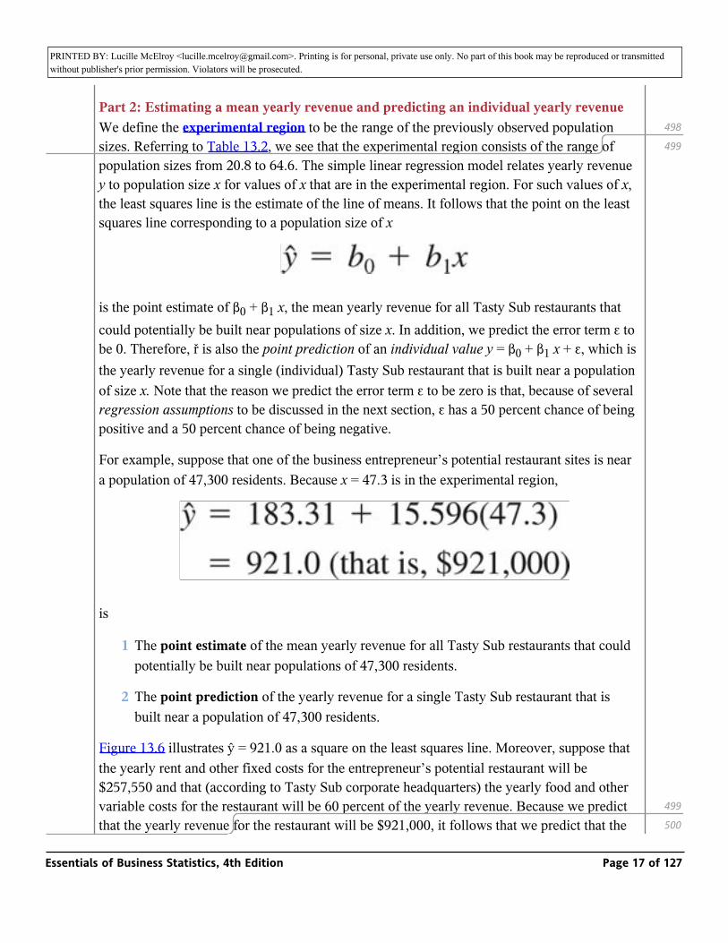
For example, suppose that one of the business entrepreneur’s potential restaurant sites is near a population of 47,300 residents. Because x = 47.3 is in the experimental region,
is
1 The point estimate of the mean yearly revenue for all Tasty Sub restaurants that could potentially be built near populations of 47,300 residents.
2 The point prediction of the yearly revenue for a single Tasty Sub restaurant that is built near a population of 47,300 residents.
Figure 13.6 illustrates ŷ = 921.0 as a square on the least squares line. Moreover, suppose that the yearly rent and other fixed costs for the entrepreneur’s potential restaurant will be $257,550 and that (according to Tasty Sub corporate headquarters) the yearly food and other variable costs for the restaurant will be 60 percent of the yearly revenue. Because we predict that the yearly revenue for the restaurant will be $921,000, it follows that we predict that the yearly total operating cost for the restaurant will be $257,550 + .6($921,000) = $810,150. In
498
499
499
500
Essentials of Business Statistics, 4th Edition Page 17 of 127

PRINTED BY: Lucille McElroy <[email protected]>. Printing is for personal, private use only. No part of this book may be reproduced or transmitted without publisher's prior permission. Violators will be prosecuted.that the yearly revenue for the restaurant will be $921,000, it follows that we predict that the
yearly total operating cost for the restaurant will be $257,550 + .6($921,000) = $810,150. In addition, if we subtract this predicted yearly operating cost from the predicted yearly revenue of $921,000, we predict that the yearly profit for the restaurant will be $110,850. Of course, these predictions are point predictions. In Section 13.4 we will predict the restaurant’s yearly revenue and profit with confidence.
FIGURE 13.6: Point Estimation and Point Prediction, and the Danger of Extrapolation
_
Essentials of Business Statistics, 4th Edition Page 18 of 127

PRINTED BY: Lucille McElroy <[email protected]>. Printing is for personal, private use only. No part of this book may be reproduced or transmitted without publisher's prior permission. Violators will be prosecuted.
_
To conclude this example, note that Figure 13.6 illustrates the potential danger of using the least squares line to predict outside the experimental region. In the figure, we extrapolate the least squares line beyond the experimental region to obtain a prediction for a population size of x = 90. As shown in Figure 13.6, for values of x in the experimental region (that is, between 20.8 and 64.6) the observed values of y tend to increase in a straight-line fashion as the values of x increase. However, for population sizes greater than x = 64.6, we have no data to tell us whether the relationship between y and x continues as a straight-line relationship or, possibly, becomes a curved relationship. If, for example, this relationship becomes the sort of curved relationship shown in Figure 13.6, then extrapolating the straight-line prediction equation to obtain a prediction for x = 90 would overestimate mean yearly revenue (see Figure 13.6).
The previous example illustrates that when we are using a least squares regression line, we should not estimate a mean value or predict an individual value unless the corresponding value of x is in the experimental region—the range of the previously observed values of x. Often the value x = 0 is not in the experimental region. In such a situation, it would not be appropriate to interpret the y -intercept b0 as the estimate of the mean value of y when x equals 0. For example, consider the Tasty Sub Shop problem. Figure 13.6 illustrates that the population size x = 0 is not in the experimental region. Therefore, it would not be appropriate to use β0 = 183.31 as the point estimate of the mean yearly revenue for all Tasty Sub restaurants that could potentially be built near populations of zero residents. Because it is not meaningful to interpret the y -intercept in many regression situations, we often omit such interpretations.
We now present a general procedure for estimating a mean value and predicting an individual value:
Point Estimation and Point Prediction in Simple Linear Regression
Let β0 and β1, be the least squares point estimates of the y -intercept β0 and the slope β1 in the simple linear regression model, and suppose that x0, a specified value of the independent variable x, is inside the experimental region. Then
1 is the point estimate of the mean value of the dependent variable when the value of the independent variable is x0.
13.3.2.3
Essentials of Business Statistics, 4th Edition Page 19 of 127

PRINTED BY: Lucille McElroy <[email protected]>. Printing is for personal, private use only. No part of this book may be reproduced or transmitted without publisher's prior permission. Violators will be prosecuted.independent variable is x0.
2 is the point prediction of an individual value of the dependent variable when the value of the independent variable is x0. Here we predict the error term to be 0.
Exercises for Section 13.1CONCEPTS
13.1 What is the least squares regression line, and what are the least squares point estimates?
13.2 Why is it dangerous to extrapolate outside the experimental region?
METHODS AND APPLICATIONS
In Exercises 13.3 through 13.8 we present six data sets involving a dependent variable y and an independent variable x. For each data set, assume that the simple linear regression model
relates y to x.
13.3 THE FUEL CONSUMPTION CASE _ FuelCon1
On the next page we give the average hourly outdoor temperature (x) in a city during a week and the city’s natural gas consumption (y) during the week for each of eight weeks (the temperature readings are expressed in degrees Fahrenheit and the natural gas consumptions are expressed in millions of cubic feet of natural gas—denoted MMcf). The output to the right of the data is obtained when MINITAB is used to fit a least squares line to the natural gas (fuel) consumption data.
500
501
13.3.2.4
Essentials of Business Statistics, 4th Edition Page 20 of 127
PRINTED BY: Lucille McElroy <[email protected]>. Printing is for personal, private use only. No part of this book may be reproduced or transmitted without publisher's prior permission. Violators will be prosecuted.
a Find the least squares point estimates β0 and β1 on the computer output and report their values. Interpret b0 and b1. Is an average hourly temperature of 0°F in the experimental region? What does this say about the interpretation of b0 ?
b Use the facts that SSxy = −179.6475; SSxx = 1,404.355; _ = 10.2125; and _ = 43.98 to hand calculate (within rounding) b0 and b1.
yx
c Use the least squares line to compute a point estimate of the mean fuel consumption for all weeks having an average hourly temperature of 40°F and a point prediction of the fuel consumption for an individual week having an average hourly temperature of 40°F.
13.4 THE STARTING SALARY CASE _ StartSal
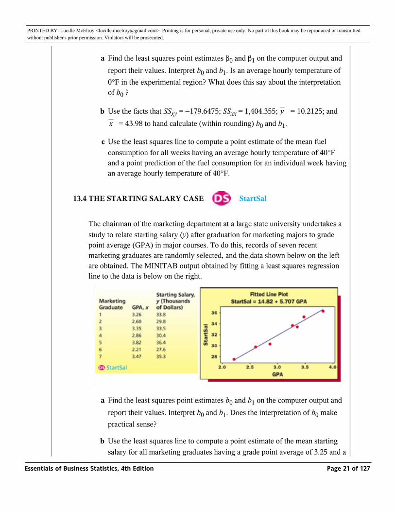
The chairman of the marketing department at a large state university undertakes a study to relate starting salary (y) after graduation for marketing majors to grade point average (GPA) in major courses. To do this, records of seven recent marketing graduates are randomly selected, and the data shown below on the left are obtained. The MINITAB output obtained by fitting a least squares regression line to the data is below on the right.
a Find the least squares point estimates b0 and b1 on the computer output and report their values. Interpret b0 and b1. Does the interpretation of b0 make practical sense?
b Use the least squares line to compute a point estimate of the mean starting salary for all marketing graduates having a grade point average of 3.25 and a point prediction of the starting salary for an individual marketing graduate
Essentials of Business Statistics, 4th Edition Page 21 of 127

PRINTED BY: Lucille McElroy <[email protected]>. Printing is for personal, private use only. No part of this book may be reproduced or transmitted without publisher's prior permission. Violators will be prosecuted.salary for all marketing graduates having a grade point average of 3.25 and a
point prediction of the starting salary for an individual marketing graduate having a grade point average of 3.25.
13.5 THE SERVICE TIME CASE _ SrvcTime
Accu-Copiers, Inc., sells and services the Accu-500 copying machine. As part of its standard service contract, the company agrees to perform routine service on this copier. To obtain information about the time it takes to perform routine service, Accu-Copiers has collected data for 11 service calls. The data and Excel output from fitting a least squares regression line to the data follow on the next page.
a Find the least squares point estimates b0 and b11 on the computer output and report their values. Interpret b0 and b1. Does the interpretation of b0 make practical sense?
b Use the least squares line to compute a point estimate of the mean time to service four copiers and a point prediction of the time to service four copiers on a single call.
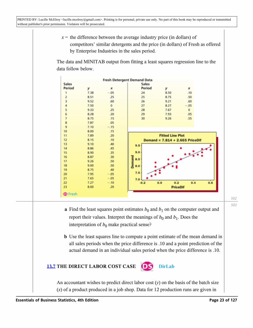
13.6 THE FRESH DETERGENT CASE _ Fresh
Enterprise Industries produces Fresh, a brand of liquid laundry detergent. In order to study the relationship between price and demand for the large bottle of Fresh, the company has gathered data concerning demand for Fresh over the last 30 sales periods (each sales period is four weeks). Here, for each sales period,
y = demand for the large bottle of Fresh (in hundreds of thousands of bottles) in the sales period, and
501
502
Essentials of Business Statistics, 4th Edition Page 22 of 127
PRINTED BY: Lucille McElroy <[email protected]>. Printing is for personal, private use only. No part of this book may be reproduced or transmitted without publisher's prior permission. Violators will be prosecuted.the sales period, and
x = the difference between the average industry price (in dollars) of competitors’ similar detergents and the price (in dollars) of Fresh as offered by Enterprise Industries in the sales period.
The data and MINITAB output from fitting a least squares regression line to the data follow below.
a Find the least squares point estimates b0 and b1 on the computer output and report their values. Interpret the meanings of b0 and b1. Does the interpretation of b0 make practical sense?
b Use the least squares line to compute a point estimate of the mean demand in all sales periods when the price difference is .10 and a point prediction of the actual demand in an individual sales period when the price difference is .10.
13.7 THE DIRECT LABOR COST CASE _ DirLab
An accountant wishes to predict direct labor cost (y) on the basis of the batch size (x) of a product produced in a job shop. Data for 12 production runs are given in the table below, along with the Excel output from fitting a least squares regression
502
503
Essentials of Business Statistics, 4th Edition Page 23 of 127

PRINTED BY: Lucille McElroy <[email protected]>. Printing is for personal, private use only. No part of this book may be reproduced or transmitted without publisher's prior permission. Violators will be prosecuted.(x) of a product produced in a job shop. Data for 12 production runs are given in
the table below, along with the Excel output from fitting a least squares regression line to the data.
Essentials of Business Statistics, 4th Edition Page 24 of 127

PRINTED BY: Lucille McElroy <[email protected]>. Printing is for personal, private use only. No part of this book may be reproduced or transmitted without publisher's prior permission. Violators will be prosecuted.
a By using the formulas illustrated in Example 13.2 (see page 497) and the data provided, verify that (within rounding) b0 = 18.488 and b1 = 10.146, as shown on the Excel output.
b Interpret the meanings of b0 and b1. Does the interpretation of b0 make practical sense?
c Write the least squares prediction equation.
d Use the least squares line to obtain a point estimate of the mean direct labor cost for all batches of size 60 and a point prediction of the direct labor cost for an individual batch of size 60.
13.8 THE REAL ESTATE SALES PRICE CASE _ RealEst
A real estate agency collects data concerning y = the sales price of a house (in thousands of dollars), and x = the home size (in hundreds of square feet). The data are given in the table below. The MINITAB output from fitting a least squares regression line to the data is on the next page.
503
Essentials of Business Statistics, 4th Edition Page 25 of 127

PRINTED BY: Lucille McElroy <[email protected]>. Printing is for personal, private use only. No part of this book may be reproduced or transmitted without publisher's prior permission. Violators will be prosecuted.
a By using the formulas illustrated in Example 13.2 (see page 497) and the data provided, verify that (within rounding) b0 = 48.02 and b1 = 5.700, as shown on the MINITAB output.
b Interpret the meanings of b0 and b1. Does the interpretation of b0 make practical sense?
c Write the least squares prediction equation.
d Use the least squares line to obtain a point estimate of the mean sales price of all houses having 2,000 square feet and a point prediction of the sales price of an individual house having 2,000 square feet.
_ Describe the assumptions behind simple linear regression and calculate the
standard error.
504
Essentials of Business Statistics, 4th Edition Page 26 of 127

PRINTED BY: Lucille McElroy <[email protected]>. Printing is for personal, private use only. No part of this book may be reproduced or transmitted without publisher's prior permission. Violators will be prosecuted.
13.2: Model Assumptions and the Standard Error
Model assumptions
In order to perform hypothesis tests and set up various types of intervals when using the simple linear regression model
we need to make certain assumptions about the error term ε. At any given value of x, there is a population of error term values that could potentially occur. These error term values describe the different potential effects on y of all factors other than the value of x. Therefore, these error term values explain the variation in the y values that could be observed when the independent variable is x. Our statement of the simple linear regression model assumes that µy, the mean of the population of all y values that could be observed when the independent variable is x, is β0 + β1 x. This model also implies that ε = y − (β0 + β1 x), so this is equivalent to assuming that the mean of the corresponding population of potential error term values is 0. In total, we make four assumptions (called the regression assumptions) about the simple linear regression model. These assumptions can be stated in terms of potential y values or, equivalently, in terms of potential error term values. Following tradition, we begin by stating these assumptions in terms of potential error term values:
The Regression Assumptions
1 At any given value of x, the population of potential error term values has a mean equal to 0.
2 Constant Variance Assumption At any given value of x, the population of potential error term values has a variance that does not depend on the value of x. That is, the different populations of potential error term values corresponding to different values of x have equal variances. We denote the constant variance as σ2.
3 Normality Assumption
At any given value of x, the population of potential error term values has a normal distribution.
4 Independence Assumption
13.4
13.4.1
13.4.1.1
Essentials of Business Statistics, 4th Edition Page 27 of 127

PRINTED BY: Lucille McElroy <[email protected]>. Printing is for personal, private use only. No part of this book may be reproduced or transmitted without publisher's prior permission. Violators will be prosecuted.4 Independence Assumption
Any one value of the error term ε is statistically independent of any other value of ε. That is, the value of the error term ε corresponding to an observed value of y is statistically independent of the value of the error term corresponding to any other observed value of y.
Taken together, the first three assumptions say that, at any given value of x, the population of potential error term values is normally distributed with mean zero and a varianceσ2 that does not depend on the value of x . Because the potential error term values cause the variation in the potential y values, these assumptions imply that the population of all y values that could be observed when the independent variable is x is normally distributed with mean β0 + β1 x x and a
varianceσ2 that does not depend on x . These three assumptions are illustrated in Figure 13.7 in the context of the Tasty Sub Shop problem. Specifically, this figure depicts the populations of yearly revenues corresponding to two values of the population size x—32.3 and 61.7. Note that these populations are shown to be normally distributed with different means (each of which is on the line of means) and with the same variance (or spread).
FIGURE 13.7: An Illustration of the Model Assumptions
The independence assumption is most likely to be violated when time series data are being utilized in a regression study. For example, the fuel consumption data in Exercise 13.3 are time series data. Intuitively, the independence assumption says that there is no pattern of positive error terms being followed (in time) by other positive error terms, and there is no pattern of positive error terms being followed by negative error terms. That is, there is no pattern of higher-than-average y values being followed by other higher-than-average y values, and there is no pattern of
504
505
Essentials of Business Statistics, 4th Edition Page 28 of 127

PRINTED BY: Lucille McElroy <[email protected]>. Printing is for personal, private use only. No part of this book may be reproduced or transmitted without publisher's prior permission. Violators will be prosecuted.error terms being followed by negative error terms. That is, there is no pattern of higher-than-
average y values being followed by other higher-than-average y values, and there is no pattern of higher-than-average y values being followed by lower-than-average y values.
It is important to point out that the regression assumptions very seldom, if ever, hold exactly in any practical regression problem. However, it has been found that regression results are not extremely sensitive to mild departures from these assumptions. In practice, only pronounced departures from these assumptions require attention. In Section 13.9 we show how to check the regression assumptions. Prior to doing this, we will suppose that the assumptions are valid in our examples.
In Section 13.1 we stated that, when we predict an individual value of the dependent variable, we predict the error term to be 0. To see why we do this, note that the regression assumptions state that, at any given value of the independent variable, the population of all error term values that can potentially occur is normally distributed with a mean equal to 0. Since we also assume that successive error terms (observed over time) are statistically independent, each error term has a 50 percent chance of being positive and a 50 percent chance of being negative. Therefore, it is reasonable to predict any particular error term value to be 0.
The mean square error and the standard error
To present statistical inference formulas in later sections, we need to be able to compute point estimates of σ2 and σ the constant variance and standard deviation of the error term populations. The point estimate of σ2 is called the mean square error and the point estimate of σ is called the standard error. In the following box, we show how to compute these estimates:
The Mean Square Error and the Standard Error
If the regression assumptions are satisfied and SSE is the sum of squared residuals:
1 The point estimate of σ2 is the mean square error
2 The point estimate of σ is the standard error
505
506
13.4.2
13.4.2.1
Essentials of Business Statistics, 4th Edition Page 29 of 127

PRINTED BY: Lucille McElroy <[email protected]>. Printing is for personal, private use only. No part of this book may be reproduced or transmitted without publisher's prior permission. Violators will be prosecuted.
In order to understand these point estimates, recall that σ2 is the variance of the population of y values (for a given value of x) around the mean value µy . Because ŷ is the point estimate of this mean, it seems natural to use
to help construct a point estimate of σ2. We divide SSE by n − 2 because it can be proven that doing so makes the resulting s2 an unbiased point estimate of σ2. Here we call n − 2 the number of degrees of freedom associated with SSE.
EXAMPLE 13.3: The Tasty Sub Shop Case
Consider the Tasty Sub Shop situation, and recall that in Table 13.2 (page 498) we have calculated the sum of squared residuals to be SSE = 30,460.21. It follows, because we have observed n = 10 yearly revenues, that the point estimate of σ2 is the mean square error
This implies that the point estimate of σ is the standard error
To conclude this section, note that in optional Section 13.10 we present a shortcut formula for calculating SSE. The reader may study Section 13.10 now or at any later point.
Exercises for Section 13.2
_
CONCEPTS
13.9 What four assumptions do we make about the simple linear regression model?
13.4.2.213.4.2.2
13.4.2.3
Essentials of Business Statistics, 4th Edition Page 30 of 127

PRINTED BY: Lucille McElroy <[email protected]>. Printing is for personal, private use only. No part of this book may be reproduced or transmitted without publisher's prior permission. Violators will be prosecuted.13.9 What four assumptions do we make about the simple linear regression model?
13.10 What is estimated by the mean square error, and what is estimated by the standard error?
METHODS AND APPLICATIONS
13.11 THE FUEL CONSUMPTION CASE _ FuelCon1
When a least squares line is fit to the 8 observations in the fuel consumption data, we obtain SSE = 2.568. Calculate s 2 and s.
13.12 THE STARTING SALARY CASE _ StartSal
When a least squares line is fit to the 7 observations in the starting salary data, we obtain SSE = 1.438. Calculate s 2 and s.
13.13 THE SERVICE TIME CASE _ SrvcTime
When a least squares line is fit to the 11 observations in the service time data, we obtain SSE = 191.7017. Calculate s 2 and s.
13.14 THE FRESH DETERGENT CASE _ Fresh
When a least squares line is fit to the 30 observations in the Fresh detergent data, we obtain SSE = 2.806. Calculate s 2 and s.
13.15 THE DIRECT LABOR COST CASE _ DirLab
When a least squares line is fit to the 12 observations in the labor cost data, we obtain SSE = 746.7624. Calculate s 2 and s.
13.16 THE REAL ESTATE SALES PRICE CASE _ RealEst
506
507
Essentials of Business Statistics, 4th Edition Page 31 of 127

PRINTED BY: Lucille McElroy <[email protected]>. Printing is for personal, private use only. No part of this book may be reproduced or transmitted without publisher's prior permission. Violators will be prosecuted.
THE REAL ESTATE SALES PRICE CASE _ RealEst
When a least squares line is fit to the 10 observations in the real estate sales price data, we obtain SSE = 896.8. Calculate s2 and s.
13.17 Ten sales regions of equal sales potential for a company were randomly selected. The advertising expenditures (in units of $10,000) in these 10 sales regions were purposely set during July of last year at, respectively, 5, 6, 7, 8, 9, 10, 11, 12, 13 and 14. The sales volumes (in units of $10,000) were then recorded for the 10 sales regions and found to be, respectively, 89, 87, 98, 110, 103, 114, 116, 110, 126, and 130. Assuming that the simple linear regression model is appropriate, it can be shown that b0 = 66.2121, b1 = 4.4303, and SSE = 222.8242. Calculate s 2
and s. _ SalesPlot
13.3: Testing the Significance of the Slope and y -Intercept
_ Test the significance of the slope and y -Intercept.
Testing the significance of the slope
A simple linear regression model is not likely to be useful unless there is a significant relationship between y and x . In order to judge the significance of the relationship between y and x, we test the null hypothesis
which says that there is no change in the mean value of y associated with an increase in x, versus the alternative hypothesis
which says that there is a (positive or negative) change in the mean value of y associated with an increase in x. It would be reasonable to conclude that x is significantly related to y if we can be quite certain that we should reject H0 in favor of Ha .
13.5
13.5.1
Essentials of Business Statistics, 4th Edition Page 32 of 127

PRINTED BY: Lucille McElroy <[email protected]>. Printing is for personal, private use only. No part of this book may be reproduced or transmitted without publisher's prior permission. Violators will be prosecuted.quite certain that we should reject H0 in favor of Ha .
In order to test these hypotheses, recall that we compute the least squares point estimate b1 of the true slope β1 by using a sample of n observed values of the dependent variable y. Different samples of n observed y values would yield different values of the least squares point estimate b1. It can be shown that, if the regression assumptions hold, then the population of all possible values of b1 is normally distributed with a mean of β1 and with a standard deviation of
The standard error s is the point estimate of σ, so it follows that a point estimate of σb 1 is
which is called the standard error of the estimate b1. Furthermore, if the regression assumptions hold, then the population of all values of
has a t distribution with n − 2 degrees of freedom. It follows that, if the null hypothesis H0 : β1 = 0 is true, then the population of all possible values of the test statistic
has a t distribution with n − 2 degrees of freedom. Therefore, we can test the significance of the regression relationship as follows: 507
Essentials of Business Statistics, 4th Edition Page 33 of 127

PRINTED BY: Lucille McElroy <[email protected]>. Printing is for personal, private use only. No part of this book may be reproduced or transmitted without publisher's prior permission. Violators will be prosecuted.regression relationship as follows:
Testing the Significance of the Regression Relationship: Testing the Significance of the Slope
Here ta /2, ta, and all p -values are based on n − 2 degrees of freedom. If we can reject H0 : β1 = 0 at a given value of α, then we conclude that the slope (or, equivalently, the regression relationship) is significant at the a level.
We usually use the two-sided alternative Ha : β1 ≠ 0 for this test of significance. However, sometimes a one-sided alternative is appropriate. For example, in the Tasty Sub Shop problem we can say that if the slope β1 is not 0, then it must be positive. A positive β1 would say that mean yearly revenue increases as the population size x increases. Because of this, it would be appropriate to decide that x is significantly related to y if we can reject H0 : β1 = 0 in favor of the one-sided alternative Ha : β1 > 0. Although this test would be slightly more effective than the usual two tailed test, there is little practical difference between using the one tailed or two tailed test. Furthermore, computer packages (such as Excel and MINITAB) present results for the two tailed test. For these reasons we will emphasize the two tailed test in future discussions.
It should also be noted that
1 If we can decide that the slope is significant at the .05 significance level, then we have concluded that x is significantly related to y by using a test that allows only a .05 probability of concluding that x is significantly related to y when it is not. This is usually regarded as strong evidence that the regression relationship is significant.
2 If we can decide that the slope is significant at the .01 significance level, this is usually regarded as very strong evidence that the regression relationship is significant.
507
50813.5.1.1
Essentials of Business Statistics, 4th Edition Page 34 of 127
PRINTED BY: Lucille McElroy <[email protected]>. Printing is for personal, private use only. No part of this book may be reproduced or transmitted without publisher's prior permission. Violators will be prosecuted.regarded as very strong evidence that the regression relationship is significant.
3 The smaller the significance level α at which H0 can be rejected, the stronger is the evidence that the regression relationship is significant.
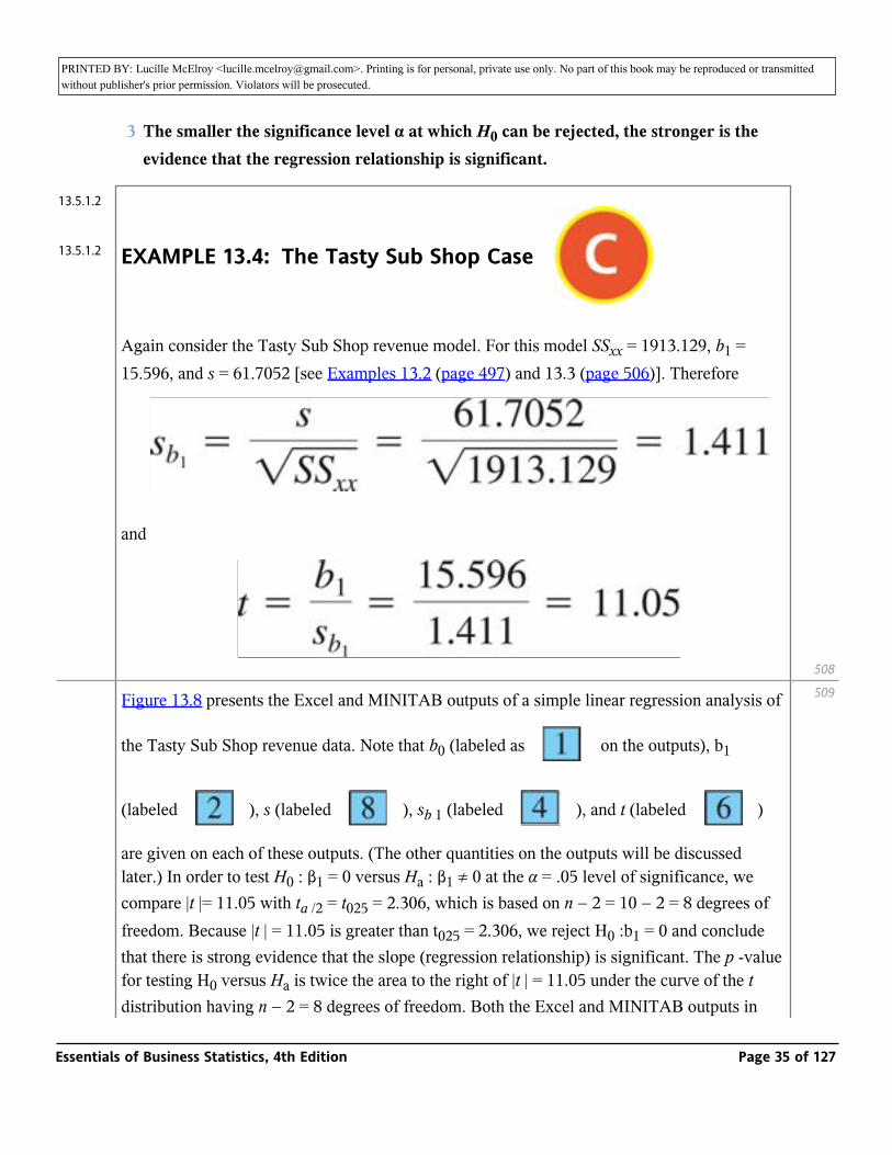
EXAMPLE 13.4: The Tasty Sub Shop Case _
Again consider the Tasty Sub Shop revenue model. For this model SSxx = 1913.129, b1 = 15.596, and s = 61.7052 [see Examples 13.2 (page 497) and 13.3 (page 506)]. Therefore
and
Figure 13.8 presents the Excel and MINITAB outputs of a simple linear regression analysis of
the Tasty Sub Shop revenue data. Note that b0 (labeled as _ on the outputs), b1
(labeled _ ), s (labeled _ ), sb 1 (labeled _ ), and t (labeled _ )
are given on each of these outputs. (The other quantities on the outputs will be discussed later.) In order to test H0 : β1 = 0 versus Ha : β1 ≠ 0 at the α = .05 level of significance, we compare |t |= 11.05 with ta /2 = t025 = 2.306, which is based on n − 2 = 10 − 2 = 8 degrees of freedom. Because |t | = 11.05 is greater than t025 = 2.306, we reject H0 :b1 = 0 and conclude that there is strong evidence that the slope (regression relationship) is significant. The p -value for testing H0 versus Ha is twice the area to the right of |t | = 11.05 under the curve of the t distribution having n − 2 = 8 degrees of freedom. Both the Excel and MINITAB outputs in
Figure 13.8 tell us that this p -value is less than .001 (see _ on the outputs). It follows
508
509
13.5.1.2
13.5.1.2
Essentials of Business Statistics, 4th Edition Page 35 of 127

PRINTED BY: Lucille McElroy <[email protected]>. Printing is for personal, private use only. No part of this book may be reproduced or transmitted without publisher's prior permission. Violators will be prosecuted.distribution having n − 2 = 8 degrees of freedom. Both the Excel and MINITAB outputs in
Figure 13.8 tell us that this p -value is less than .001 (see _ on the outputs). It follows
that we can reject H0 in favor of Ha at level of significance .05, .01, or .001, which implies that we have extremely strong evidence that the regression relationship between x and y is significant.
FIGURE 13.8: Excel and MINITAB Outputs of a Simple Linear Regression Analysis of the Tasty Sub Shop Revenue Data
509
Essentials of Business Statistics, 4th Edition Page 36 of 127

PRINTED BY: Lucille McElroy <[email protected]>. Printing is for personal, private use only. No part of this book may be reproduced or transmitted without publisher's prior permission. Violators will be prosecuted.
A Confidence Interval for the Slope
If the regression assumptions hold, a 100(1 − α) percent confidence interval for the true slope β1 is [b1 ± tα/2 sbi ]. Here tα/2 is based on n— 2 degrees of freedom.
EXAMPLE 13.5: The Tasty Sub Shop Case _
The Excel and MINITAB outputs in Figure 13.8 tell us that b1 = 15.596 and sb1 = 1.411. Thus, for instance, because t.025 based on n - 2 = 10 - 2 = 8 degrees of freedom equals 2.306, a 95 percent confidence interval for β1 is
(where we have used more decimal place accuracy than shown to obtain the final result). This interval says we are 95 percent confident that, if the population size increases by one thousand residents, then mean yearly revenue will increase by at least $12,342 and by at most $18,849. Also, because the 95 percent confidence interval for β1 does not contain 0, we can reject H0 : β1 = 0 in favor of Ha : ≠ 0 at level of significance .05. Note that the 95 percent confidence interval for β1 is given on the Excel output but not on the MINITAB output (see Figure 13.8).
Testing the significance of the y-intercept
We can also test the significance of the y-intercept β0. We do this by testing the null hypothesis H0 : β0 = 0 versus the alternative hypothesis Ha : β0 ≠ 0. If we can reject H0 in favor of Ha by setting the probability of a Type I error equal toα, we conclude that the interceptβ0 is significant at the β level. To carry out the hypothesis test, we use the test statistic
509
51013.5.1.3
13.5.1.4
13.5.1.4
13.5.2
Essentials of Business Statistics, 4th Edition Page 37 of 127
PRINTED BY: Lucille McElroy <[email protected]>. Printing is for personal, private use only. No part of this book may be reproduced or transmitted without publisher's prior permission. Violators will be prosecuted.
Here the critical value and p-value conditions for rejecting H0 are the same as those given previously for testing the significance of the slope, except that t is calculated as b0 /sb0. For example, if we consider the Tasty Sub Shop problem and the Excel and MINITAB outputs in Figure 13.8, we see that b0 = 183.31, sb0 = 64.27, t = 2.85, and p-value = .021. Because t = 2.85 > t025 = 2.306 and p-value < .05, we can reject H0 : ft = 0 in favor of Ha : ft ≠ 0 at the .05 level of significance. This provides strong evidence that the y-intercept ft of the line of means does not equal 0 and thus is significant. Therefore, we should include ft in the Tasty Sub Shop revenue model.
In general, if we fail to conclude that the intercept is significant at a level of significance of .05, it might be reasonable to drop the y -intercept from the model. However, it is common practice to include the y-intercept whether or not H0 : β0 = 0 is rejected. In fact, experience suggests that it is definitely safest, when in doubt, to include the intercept β0.
Exercises for Section 13.3CONCEPTS
_
13.18 What do we conclude if we can reject H0 : β0 = 0 in favor of Ha : β0 ≠ 0 by setting
a α equal to .05?
b α equal to .01?
13.19 Give an example of a practical application of the confidence interval for β1.
METHODS AND APPLICATIONS
In Exercises 13.20 through 13.25, we refer to Excel and MINITAB outputs of simple linear regression analyses of the data sets related to the six case studies introduced in the exercises for Section 13.1. Using the appropriate output for each case study,
a Find the least squares point estimates b0 and b1 of β0 and β1 on the output and report their values.
13.5.2.1
Essentials of Business Statistics, 4th Edition Page 38 of 127
PRINTED BY: Lucille McElroy <[email protected]>. Printing is for personal, private use only. No part of this book may be reproduced or transmitted without publisher's prior permission. Violators will be prosecuted.output and report their values.
b Find SSE and s on the computer output and report their values.
c Find sb 1 and the t statistic for testing the significance of the slope on the output and report their values. Show (within rounding) how t has been calculated by using b1 and sb 1 from the computer output.
d Using the t statistic and appropriate critical value, test H0 : β1 = 0 versus Ha : β1 + 0 by setting a equal to .05. Is the slope (regression relationship) significant at the .05 level?
e Using the t statistic and appropriate critical value, test H0 : β1 = 0 versus Ha : β1 ≠ 0 by setting a equal to .01. Is the slope (regression relationship) significant at the .01 level?
f Find the p-value for testing H0 : β0 = 0 versus Ha : β0 ≠ 0 on the output and report its value. Using the p-value, determine whether we can reject H0 by setting a equal to .10, .05, .01, and .001. How much evidence is there that the slope (regression relationship) is significant?
g Calculate the 95 percent confidence interval for β1 using numbers on the output. Interpret the interval.
h Calculate the 99 percent confidence interval for β1 using numbers on the output.
i Find sb0 and the t statistic for testing the significance of the y intercept on the output and report their values. Show (within rounding) how t has been calculated by using b0 and sb0 from the computer output.
j Find the p-value for testing H0 :β0 = 0 versus Ha : β0 ≠0 on the computer output and report its value. Using the p-value, determine whether we can reject H0 by setting a equal to .10, .05, .01, and .001. What do you conclude about the significance of the y intercept?
510
511
Essentials of Business Statistics, 4th Edition Page 39 of 127

PRINTED BY: Lucille McElroy <[email protected]>. Printing is for personal, private use only. No part of this book may be reproduced or transmitted without publisher's prior permission. Violators will be prosecuted.intercept?
k Using the data set and s from the computer output, hand calculate (within rounding) SSxx, sb0, and sb1.
13.20 THE FUEL CONSUMPTION CASE _ FuelCon1
The Excel and MINITAB outputs of a simple linear regression analysis of the data set for this case (see Exercise 13.3 on page 500) are given in Figures 13.9 and 13.10. Labeled Excel and MINITAB outputs are on page 509 in Figure 13.8. Use whichever package is taught in your class.
FIGURE 13.9: Excel Output of a Simple Linear Regression Analysis of the Fuel Consumption Data
FIGURE 13.10: MINITAB Output of a Simple Linear Regression Analysis of the Fuel Consumption Data
Essentials of Business Statistics, 4th Edition Page 40 of 127
PRINTED BY: Lucille McElroy <[email protected]>. Printing is for personal, private use only. No part of this book may be reproduced or transmitted without publisher's prior permission. Violators will be prosecuted.
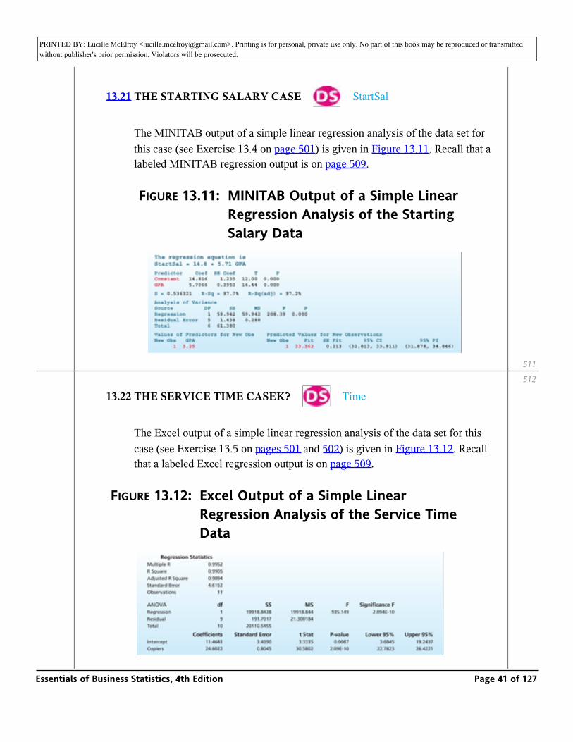
13.21 THE STARTING SALARY CASE _ StartSal
The MINITAB output of a simple linear regression analysis of the data set for this case (see Exercise 13.4 on page 501) is given in Figure 13.11. Recall that a labeled MINITAB regression output is on page 509.
FIGURE 13.11: MINITAB Output of a Simple Linear Regression Analysis of the Starting Salary Data
13.22 THE SERVICE TIME CASEK? _ Time
The Excel output of a simple linear regression analysis of the data set for this case (see Exercise 13.5 on pages 501 and 502) is given in Figure 13.12. Recall that a labeled Excel regression output is on page 509.
FIGURE 13.12: Excel Output of a Simple Linear Regression Analysis of the Service Time Data
511
512
Essentials of Business Statistics, 4th Edition Page 41 of 127

PRINTED BY: Lucille McElroy <[email protected]>. Printing is for personal, private use only. No part of this book may be reproduced or transmitted without publisher's prior permission. Violators will be prosecuted.
13.23 THE FRESH DETERGENT CASE _ Fresh
The MINITAB output of a simple linear regression analysis of the data set for this case (see Exercise 13.6 on page 502) is given in Figure 13.13. Recall that a labeled MINITAB regression output is on page 509.
FIGURE 13.13: MINITAB Output of a Simple Linear Regression Analysis of the Fresh Detergent Demand Data
13.24 THE DIRECT LABOR COST CASE _ DirLab
The Excel output of a simple linear regression analysis of the data set for this case (see Exercise 13.7 on page 503) is given in Figure 13.14. Recall that a labeled Excel regression output is on page 509.
FIGURE 13.14: Excel Output of a Simple Linear Regression Analysis of the Direct Labor Cost Data
Essentials of Business Statistics, 4th Edition Page 42 of 127

PRINTED BY: Lucille McElroy <[email protected]>. Printing is for personal, private use only. No part of this book may be reproduced or transmitted without publisher's prior permission. Violators will be prosecuted.
13.25 THE REAL ESTATE SALES PRICE CASE _ RealEst
The MINITAB output of a simple linear regression analysis of the data set for this case (see Exercise 13.8 on page 503) is given in Figure 13.15. Recall that a labeled MINITAB regression output is on page 509.
FIGURE 13.15: MINITAB Output of a Simple Linear Regression Analysis of the Real Estate Sales Price Data
13.26 Find and interpret a 95 percent confidence interval for the slope β1 of the simple linear regression model describing the sales volume data in Exercise 13.17 (page
507). _ SalesPlot
13.27 THE FAST-FOOD RESTAURANT RATING CASE _ FastFood
In the early 1990s researchers at The Ohio State University studied consumer ratings of six fast-food restaurants: Borden Burger, Hardee’s, Burger King, McDonald’s, Wendy’s, and White Castle. Each of 406 randomly selected individuals gave each restaurant a rating of 1, 2, 3, 4, 5, or 6 on the basis of taste, and then ranked the restaurants from 1 through 6 on the basis of overall preference. In each case, 1 is the best rating and 6 the worst. The mean ratings given by the 406 individuals are given in the following table:
512
513
Essentials of Business Statistics, 4th Edition Page 43 of 127

PRINTED BY: Lucille McElroy <[email protected]>. Printing is for personal, private use only. No part of this book may be reproduced or transmitted without publisher's prior permission. Violators will be prosecuted.given by the 406 individuals are given in the following table:
Figure 13.16 gives the Excel output of a simple linear regression analysis of this data. Here, mean preference is the dependent variable and mean taste is the independent variable. Recall that a labeled Excel regression output is given on page 509.
FIGURE 13.16: Excel Output of a Simple Linear Regression Analysis of the Fast-Food Restaurant Rating Data
a Find the least squares point estimate β1 of β1 on the computer output. Report and interpret this estimate.
b Find the 95 percent confidence interval for β1 on the output. Report and interpret the interval.
513
514
Essentials of Business Statistics, 4th Edition Page 44 of 127

PRINTED BY: Lucille McElroy <[email protected]>. Printing is for personal, private use only. No part of this book may be reproduced or transmitted without publisher's prior permission. Violators will be prosecuted.
13.4: Confidence and Prediction Intervals
_ Calculate and interpret a confidence interval for a mean value and a
prediction interval for an individual value.
If the regression relationship between y and x is significant, then
is the point estimate of the mean value of y when the value of the independent variable x is x0. We have also seen that _ is the point prediction of an individual value of y when the value of the independent variable x is x0. In this section we will assess the accuracy of y as both a point estimate and a point prediction. To do this, we will find a confidence interval for the mean value of y and a prediction interval for an individual value of y.
y^
Because each possible sample of n values of the dependent variable gives values of b0 and b1 t that differ from the values given by other samples, different samples give different values of _ = _
+ _ _ . If the regression assumptions hold, a confidence interval for the mean value of y is based
on the estimated standard deviation of the normally distributed population of all possible values of _ . This estimated standard deviation is called the standard error of _ is denoted _ , and is given
by the formula
y^ b 0
b 1 x 0
y^ y^ S _y^
Here, s is the standard error (see Section 13.2), _ is the average of the n previously observed values
of x, and _ = Σ_ − ( Σ_ _ / n .
x
S S x x x i2 ( x i ))
2
/As explained above, a confidence interval for the mean value of y is based on the standard error _ .
A prediction interval for an individual value of y is based on a more complex standard error: the estimated standard deviation of the population of all possible values of y − _ , the prediction error
S _y
^
514
515
13.6
Essentials of Business Statistics, 4th Edition Page 45 of 127
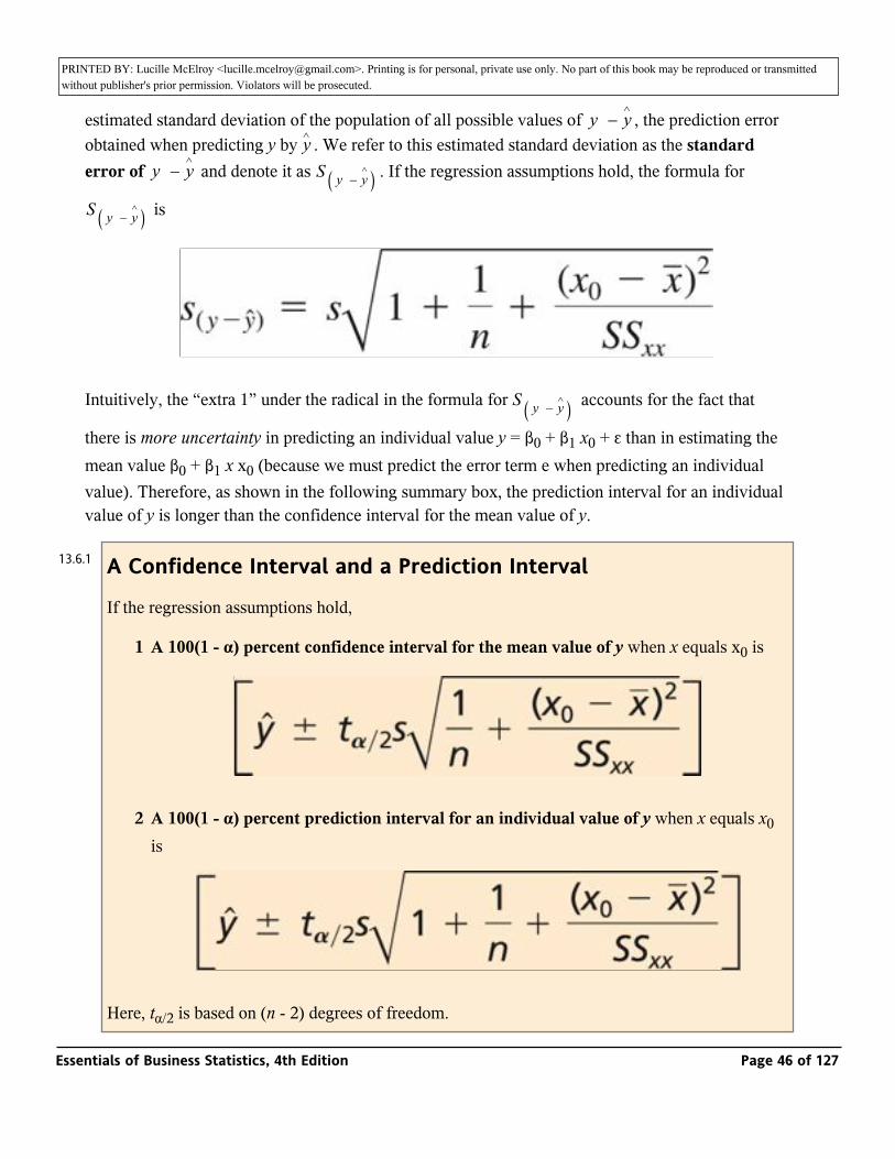
PRINTED BY: Lucille McElroy <[email protected]>. Printing is for personal, private use only. No part of this book may be reproduced or transmitted without publisher's prior permission. Violators will be prosecuted.A prediction interval for an individual value of y is based on a more complex standard error: the
estimated standard deviation of the population of all possible values of y − _ , the prediction error obtained when predicting y by _ . We refer to this estimated standard deviation as the standard error of y − _ and denote it as _ . If the regression assumptions hold, the formula for
_ is
y^
yy^ S ( y − _)( y
^ )S ( y − _)( y
^ )
Intuitively, the “extra 1” under the radical in the formula for _ accounts for the fact that
there is more uncertainty in predicting an individual value y = β0 + β1 x0 + ε than in estimating the mean value β0 + β1 x x0 (because we must predict the error term e when predicting an individual value). Therefore, as shown in the following summary box, the prediction interval for an individual value of y is longer than the confidence interval for the mean value of y.
S ( y − _)( y )
A Confidence Interval and a Prediction Interval
If the regression assumptions hold,
1 A 100(1 - α) percent confidence interval for the mean value of y when x equals x0 is
2 A 100(1 - α) percent prediction interval for an individual value of y when x equals x0 is
Here, tα/2 is based on (n - 2) degrees of freedom.
13.6.1
Essentials of Business Statistics, 4th Edition Page 46 of 127

PRINTED BY: Lucille McElroy <[email protected]>. Printing is for personal, private use only. No part of this book may be reproduced or transmitted without publisher's prior permission. Violators will be prosecuted.
The summary box tells us that both the formula for the confidence interval and the formula for the
prediction interval use the quantity 1 / n + (_ − _ _ / _ We will call this quantity the
distance value, because it is a measure of the distance between x0, the value of x for which we will make a point estimate or a point prediction, and _ , the average of the previously observed values of x. The farther that x0 is from _ , which represents the center of the experimental region, the larger is
the distance value, and thus the longer are both the confidence interval [_
± _ s_ ] and the predictiis farther from the center of the data, on interval [_
± _ s_ ]. Said another way, when x0 is farther from the center of the data,
_ = _ + _ _ is likely to be less accurate as both a point estimate and a point prediction.
/ ( x 0 x ))2
/ S S x x
xx
[ y
t α / 2 distance value ] [ y^
t α / 2 distance value ]y^ b 0 b 1 x 0
EXAMPLE 13.6: The Tasty Sub Shop Case _
In the Tasty Sub Shop problem, recall that one of the business entrepreneur’s potential sites is near a population of 47,300 residents. Also, recall that
is the point estimate of the mean yearly revenue for all Tasty Sub restaurants that could potentially be built near populations of 47,300 residents and is the point prediction of the yearly revenue for a single Tasty Sub restaurant that is built near a population of 47,300 residents. Using the information in Example 13.2 (page 497), we compute
515
516
13.6.2
13.6.2
Essentials of Business Statistics, 4th Edition Page 47 of 127

PRINTED BY: Lucille McElroy <[email protected]>. Printing is for personal, private use only. No part of this book may be reproduced or transmitted without publisher's prior permission. Violators will be prosecuted.Using the information in Example 13.2 (page 497), we compute
Since s = 61.7052(see Example 13.3 on page 506) andsince tα/2 = t.025 basedon n − 2 = 10 − 2 = 8 degrees of freedom equals 2.306, it follows that a 95 percent confidence interval for the mean yearly revenue when x = 47.3 is
This interval says we are 95 percent confident that the mean yearly revenue for all Tasty Sub restaurants that could potentially be built near populations of 47,300 residents is between $874,300 and $967,700.
Because the entrepreneur would be operating a single Tasty Sub restaurant that is built near a population of 47,300 residents, the entrepreneur is interested in obtaining a prediction interval for the yearly revenue of such a restaurant. A 95 percent prediction interval for this revenue is
Essentials of Business Statistics, 4th Edition Page 48 of 127

PRINTED BY: Lucille McElroy <[email protected]>. Printing is for personal, private use only. No part of this book may be reproduced or transmitted without publisher's prior permission. Violators will be prosecuted.
This interval says that we are 95 percent confident that the yearly revenue for a single Tasty Sub restaurant that is built near a population of 47,300 residents will be between $771,200 and $1,070,800. Moreover, recall that the yearly rent and other fixed costs for the entrepreneur’s potential restaurant will be $257,550 and that (according to Tasty Sub corporate headquarters) the yearly food and other variable costs for the restaurant will be 60 percent of the yearly revenue. Using the lower end of the 95 percent prediction interval [771.2, 1070.8], we predict that (1) the restaurant’s yearly operating cost will be $257,550 + .6($771,200) = $720,270 and (2) the restaurant’s yearly profit will be $771,200 - $720,270 = $50,930. Using the upper end of the 95 percent prediction interval [771.2, 1070.8], we predict that (1) the restaurant’s yearly
operating cost will be $257,550 + .6($1,070,800) = $900,030 and (2) the restaurant’s yearly profit will be $1,070,800 - $900,030 = $170,770. Combining the two predicted profits, it follows that we are 95 percent confident that the potential restaurant’s yearly profit will be between $50,930 and $170,770. If the entrepreneur decides that this is an acceptable range of potential yearly profits, then the entrepreneur might decide to purchase a Tasty Sub franchise for the potential restaurant site. In Chapter 14 we will use a multiple regression model to reduce the range of the predicted yearly profits for the potential Tasty Sub restaurant.
_
Below we repeat the bottom of the MINITAB output in Figure 13.8(b) on page 509. This output gives (within rounding) the point estimate and prediction _ = 921.0, the 95 percent confidence interval for the mean value of y when x equals 47.3, and the 95 percent prediction interval for an individual value of y when x equals 47.3.
y^
Although the MINITAB output does not directly give the distance value, it does give _ = s_ under the heading “SE Fit.” A little algebra shows that this implies that the
distance value equals (_ / S_ . Specifically, because sy = 20.3 and s = 61.7052, the distance
s _y^ distance value2
516
517
Essentials of Business Statistics, 4th Edition Page 49 of 127

PRINTED BY: Lucille McElroy <[email protected]>. Printing is for personal, private use only. No part of this book may be reproduced or transmitted without publisher's prior permission. Violators will be prosecuted._ = s_ under the heading “SE Fit.” A little algebra shows that this implies that the
distance value equals (_ / S_ . Specifically, because sy = 20.3 and s = 61.7052, the distance
value equals (20.3/61.7052)2 = .1082. Note that, because MINITAB rounds sŷ, this calculation of the distance value is slightly less accurate than the previous hand calculation that obtained a distance value of .1079.
_y
( S _y / ))2
To conclude this example, note that Figure 13.17 illustrates the MINITAB output of the 95 percent confidence and prediction intervals corresponding to all values of x in the experimental region. Here _ = 43.41 can be regarded as the center of the experimental region. Notice that the farther x0 is from _ = 43.41, the larger is the distance value and, therefore, the longer are the 95 percent confidence and prediction intervals. These longer intervals are undesirable because they give us less information about mean and individual values of y.
xx
FIGURE 13.17: MINITAB Output of 95% Confidence and Prediction Intervals for the Tasty Sub Shop Case
Exercises for Section 13.4CONCEPT
517
51813.6.3
Essentials of Business Statistics, 4th Edition Page 50 of 127

PRINTED BY: Lucille McElroy <[email protected]>. Printing is for personal, private use only. No part of this book may be reproduced or transmitted without publisher's prior permission. Violators will be prosecuted.
CONCEPT
_
13.28 What is the difference between a confidence interval and a prediction interval?
13.29 What does the distance value measure? How does the distance value affect a confidence or prediction interval?
METHODS AND APPLICATIONS
13.30 THE FUEL CONSUMPTION CASE _ FuelConl
The following partial MINITAB regression output for the fuel consumption data relates to predicting the city’s fuel consumption (in MMcf of natural gas) in a week that has an average hourly temperature of 40°F.
a Report (as shown on the computer output) a point estimate of and a 95 percent confidence interval for the mean fuel consumption for all weeks having an average hourly temperature of 40°F.
b Report (as shown on the computer output) a point prediction of and a 95 percent prediction interval for the fuel consumption in a single week that has an average hourly temperature of 40°F.
c Remembering that s = .6542; SSxx = 1,404.355;_ = 43.98 n = 8, hand calculate the distance value when x0 = 40. Remembering that the distance
value equals (_ / S_ , use s and _ from the computer output to calculate
(within rounding) the distance value using this formula. Note that, because MINITAB rounds sy, the first hand calculation is the more accurate calculation of the distance value.
x
( S _y / ))2
S _y
d Remembering that for the fuel consumption data b0 = 15.84 and b1 = —.1279, calculate (within rounding) the confidence interval of part a and the prediction interval of part b.
Essentials of Business Statistics, 4th Edition Page 51 of 127

PRINTED BY: Lucille McElroy <[email protected]>. Printing is for personal, private use only. No part of this book may be reproduced or transmitted without publisher's prior permission. Violators will be prosecuted.prediction interval of part b.
e Suppose that next week the city’s average hourly temperature will be 40°F. Also, suppose that the city’s natural gas company will use the point prediction _ = 10.721 and order 10.721 MMcf of natural gas to be shipped to the city by a pipeline transmission system. The company will have to pay a fine to the transmission system if the city’s actual gas useage y differs from the order of 10.721 MMcf by more than 10.5 percent—that is, is outside of the range [10.721 ± .105(10.721)] = [9.595, 11.847]. Discuss why the 95 percent prediction interval for y, [9.015, 12.427], says that y might be outside of the allowable range and thus does not make the company 95 percent confident that it will avoid paying a fine.
y^
Note: In the exercises of Chapter 14 we will use multiple regression analysis to predict y accurately enough that the company is likely to avoid paying a fine.
13.31 THE STARTING SALARY CASE _ StartSal
The following partial MINITAB regression output for the starting salary data relates to predicting the starting salary of a marketing graduate having a grade point average of 3.25.
a Report (as shown on the computer output) a point estimate of and a 95 percent confidence interval for the mean starting salary of all marketing graduates having a grade point average of 3.25.
b Report (as shown on the computer output) a point prediction of and a 95 percent prediction interval for the starting salary of an individual marketing graduate having a grade point average of 3.25.
c Remembering that s = .536321 and that the distance value equals (_ /
S_ , use sy from the computer output to hand calculate the distance value
when x = 3.25.
( S _y /))
2
Essentials of Business Statistics, 4th Edition Page 52 of 127

PRINTED BY: Lucille McElroy <[email protected]>. Printing is for personal, private use only. No part of this book may be reproduced or transmitted without publisher's prior permission. Violators will be prosecuted.when x = 3.25.
d Remembering that for the starting salary data n = 7, b0 = 14.816, and b1 = 5.7066, hand calculate (within rounding) the confidence interval of part a and the prediction interval of part b.
13.32 THE SERVICE TIME CASE _ SrvcTime
The following partial Excel add-in (MegaStat) regression output for the service time data relates to predicting service times for 1, 2, 3, 4, 5, 6, and 7 copiers.
a Report (as shown on the computer output) a point estimate of and a 95 percent confidence interval for the mean time to service four copiers.
b Report (as shown on the computer output) a point prediction of and a 95 percent prediction interval for the time to service four copiers on a single call.
c For this case: n = 11, b0 = 11.4641, b11 = 24.6022, and s = 4.615. Using this information and a distance value (called Leverage on the add-in output), hand calculate (within rounding) the confidence interval of part a and the prediction interval of part b.
d If we examine the service time data, we see that there was at least one call on which Accu-Copiers serviced each of 1, 2, 3, 4, 5, 6, and 7 copiers. The 95 percent confidence intervals for the mean service times on these calls might be used to schedule future service calls. To understand this, note that a person making service calls will (in, say, a year or more) make a very large number of service calls. Some of the person’s individual service times will be below, and some will be above, the corresponding mean service times. However, since the very large number of individual service times will average out to the mean service times, it seems fair to both the efficiency of the company and to the person making service calls to schedule service calls by using estimates of the mean service times. Therefore, suppose we wish to schedule a call to service five copiers. Examining the computer output, we see that a
518
519
Essentials of Business Statistics, 4th Edition Page 53 of 127

PRINTED BY: Lucille McElroy <[email protected]>. Printing is for personal, private use only. No part of this book may be reproduced or transmitted without publisher's prior permission. Violators will be prosecuted.estimates of the mean service times. Therefore, suppose we wish to schedule
a call to service five copiers. Examining the computer output, we see that a 95 percent confidence interval for the mean time to service five copiers is [130.753, 138.197]. Since the mean time might be 138.197 minutes, it would seem fair to allow 138 minutes to make the service call. Now suppose we wish to schedule a call to service four copiers. Determine how many minutes to allow for the service call.
13.33 THE FRESH DETERGENT CASE _ Fresh
The following partial MINITAB regression output for the Fresh detergent data relates to predicting demand for future sales periods in which the price difference will be .10 (see New Obs 1) and .25 (see New Obs2).
a Report (as shown on the computer output) a point estimate of and a 95 percent confidence interval for the mean demand for Fresh in all sales periods when the price difference is .10.
b Report (as shown on the computer output) a point prediction of and a 95 percent prediction interval for the actual demand for Fresh in an individual sales period when the price difference is .10.
c Remembering that s = .316561 and that the distance value equals (_ / S_ ,
use sy from the computer output to hand calculate the distance value when x = .10.
( S _y^ / ))2
d For this case: n = 30, b0 = 7.81409, b1 = 2.6652, and s = .316561. Using this information, and your result from part c, find 99 percent confidence and prediction intervals for mean and individual demands when x = .10.
e Repeat parts a, b, c, and d when x = .25.
13.34 THE DIRECT LABOR COST CASEBDS _ DirLab
519
520
Essentials of Business Statistics, 4th Edition Page 54 of 127
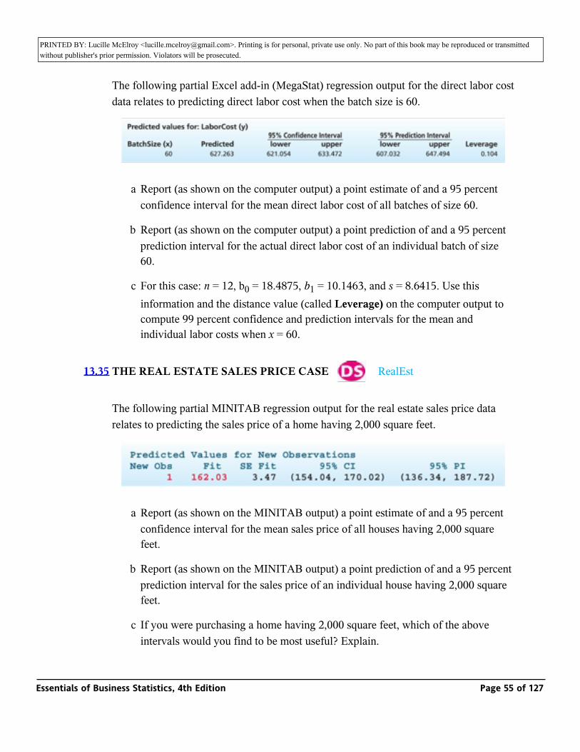
PRINTED BY: Lucille McElroy <[email protected]>. Printing is for personal, private use only. No part of this book may be reproduced or transmitted without publisher's prior permission. Violators will be prosecuted.
THE DIRECT LABOR COST CASEBDS _ DirLab
The following partial Excel add-in (MegaStat) regression output for the direct labor cost data relates to predicting direct labor cost when the batch size is 60.
a Report (as shown on the computer output) a point estimate of and a 95 percent confidence interval for the mean direct labor cost of all batches of size 60.
b Report (as shown on the computer output) a point prediction of and a 95 percent prediction interval for the actual direct labor cost of an individual batch of size 60.
c For this case: n = 12, b0 = 18.4875, b1 = 10.1463, and s = 8.6415. Use this information and the distance value (called Leverage) on the computer output to compute 99 percent confidence and prediction intervals for the mean and individual labor costs when x = 60.
13.35 THE REAL ESTATE SALES PRICE CASE_ RealEst
The following partial MINITAB regression output for the real estate sales price data relates to predicting the sales price of a home having 2,000 square feet.
a Report (as shown on the MINITAB output) a point estimate of and a 95 percent confidence interval for the mean sales price of all houses having 2,000 square feet.
b Report (as shown on the MINITAB output) a point prediction of and a 95 percent prediction interval for the sales price of an individual house having 2,000 square feet.
c If you were purchasing a home having 2,000 square feet, which of the above intervals would you find to be most useful? Explain.
Essentials of Business Statistics, 4th Edition Page 55 of 127

PRINTED BY: Lucille McElroy <[email protected]>. Printing is for personal, private use only. No part of this book may be reproduced or transmitted without publisher's prior permission. Violators will be prosecuted.intervals would you find to be most useful? Explain.
13.5: Simple Coefficients of Determination and Correlation •
The simple coefficient of determination
_ Calculate and interpret the simple coefficients of determination and
correlation.
The simple coefficient of determination is a measure of the usefulness of a simple linear regression model. To introduce this quantity, which is denoted r 2 (pronounced r squared), suppose we have observed n values of the dependent variable y. However, we choose to predict y without using a predictor (independent) variable x. In such a case the only reasonable prediction of a specific value of y, say yi, would be _ , which is simply the average of the n observed values y1, y2,..., yn. Here the error of prediction in predicting yi would be yi −_ For example, Figure 13.18(a) illustrates the prediction errors obtained for the Tasty Sub Shop revenue data when we do not use the information provided by the independent variable x, population size.
yy
FIGURE 13.18: The Reduction in the Prediction Errors Accomplished by Employing the Predictor Variable x
13.7
13.7.1
Essentials of Business Statistics, 4th Edition Page 56 of 127

PRINTED BY: Lucille McElroy <[email protected]>. Printing is for personal, private use only. No part of this book may be reproduced or transmitted without publisher's prior permission. Violators will be prosecuted.
Next, suppose we decide to employ the predictor variable x and observe the values x1, x2,. . ., xn corresponding to the observed values of y. In this case the prediction of yi is
and the error of prediction is yi − For example, Figure 13.18(b) illustrates the prediction errors obtained in the Tasty Sub Shop problem when we use the predictor variable x. Together, Figures 13.18(a) and (b) show the reduction in the prediction errors accomplished by employing the predictor variable x (and the least squares line).
Using the predictor variable x decreases the prediction error in predicting yi from (_ − _ ) to (yi
− ŷi ) or by an amount equal to( y
iy )
It can be shown that in general
The sum of squared prediction errors obtained when we do not employ the predictor variable x,
Σ_ , , is called the total variation. Intuitively, this quantity measures the total amount
of variation exhibited by the observed values of y. The sum of squared prediction errors obtained when we use the predictor variable x, Σ(yi − ŷi )2, is called the unexplained variation (this is another name for SSE). Intuitively, this quantity measures the amount of variation in the values
of y that is not explained by the predictor variable. The quantity Σ_ is called the
explained variation. Using these definitions and the above equation involving these summations, we see that
(_ − _ )( y i y )2
(_ − _ )(_y^ i y )2
It follows that the explained variation is the reduction in the sum of squared prediction errors that has been accomplished by using the predictor variable x to predict y. It also follows that
520
521
521Essentials of Business Statistics, 4th Edition Page 57 of 127

PRINTED BY: Lucille McElroy <[email protected]>. Printing is for personal, private use only. No part of this book may be reproduced or transmitted without publisher's prior permission. Violators will be prosecuted.
Intuitively, this equation implies that the explained variation represents the amount of the total variation in the observed values of y that is explained by the predictor variable x (and the simple linear regression model).
We now define the simple coefficient of determination to be
That is, r 2 is the proportion of the total variation in the n observed values of y that is explained by the simple linear regression model. Neither the explained variation nor the total variation can be negative (both quantities are sums of squares). Therefore, r 2 is greater than or equal to 0. Because the explained variation must be less than or equal to the total variation, r 2 cannot be greater than 1. The nearer r 2 is to 1, the larger is the proportion of the total variation that is explained by the model, and the greater is the utility of the model in predicting y. If the value of r 2 is not reasonably close to 1, the independent variable in the model does not provide accurate predictions of y. In such a case, a different predictor variable must be found in order to accurately predict y. It is also possible that no regression model employing a single predictor variable will accurately predict y. In this case the model must be improved by including more than one independent variable. We show how to do this in Chapter 14.
The Simple Coefficient of Determination, r 2
For the simple linear regression model
1 Total variation = Σ_(_ − _ )( y 1 y )2
2 Explained variation = Σ_(_ − _ )(_y i y )2
3 Unexplained variation = Σ_(_ − _ )( y i _y i )2
4 Total variation = Explained variation + unexplained variation
5 The simple coefficient of determination is
521
522
13.7.1.1
Essentials of Business Statistics, 4th Edition Page 58 of 127

PRINTED BY: Lucille McElroy <[email protected]>. Printing is for personal, private use only. No part of this book may be reproduced or transmitted without publisher's prior permission. Violators will be prosecuted.5 The simple coefficient of determination is
6 r 2 is the proportion of the total variation in the n observed values of the dependent variable that is explained by the simple linear regression model.
EXAMPLE 13.7: The Tasty Sub Shop Case _
For the Tasty Sub data (see Table 13.1 on page 492) we have seen that _ = (527.1 + 548.7 + ... + 1235.8)/10 = 8603.1/10 = 860.31. It follows that the total variation is
y
Furthermore, we found in Table 13.2 (page 498) that the unexplained variation is SSE = 30,460.21. Therefore, we can compute the explained variation and r 2 as follows:
This value of r 2 says that the regression model explains 93.9 percent of the total variation in the 10 observed yearly revenues.
The simple correlation coefficient, r
People often claim that two variables are correlated. For example, a college admissions officer might feel that the academic performance of college students (measured by grade point average) is correlated with the students’ scores on a standardized college entrance examination. This means that college students’ grade point averages are related to their college entrance exam scores. One measure of the relationship between two variables y and x is the simple correlation coefficient.
522
523
13.7.1.2
13.7.1.2
13.7.2
Essentials of Business Statistics, 4th Edition Page 59 of 127

PRINTED BY: Lucille McElroy <[email protected]>. Printing is for personal, private use only. No part of this book may be reproduced or transmitted without publisher's prior permission. Violators will be prosecuted.that college students’ grade point averages are related to their college entrance exam scores. One
measure of the relationship between two variables y and x is the simple correlation coefficient. We define this quantity as follows:
The Simple Correlation Coefficient
The simple correlation coefficient between y and x, denoted by r, is
where b1 is the slope of the least squares line relating y to x. This correlation coefficient measures the strength of the linear relationship between y and x.
Because r 2 is always between 0 and 1, the correlation coefficient r is between −1 and 1. A value of r near 0 implies little linear relationship between y and x. A value of r close to 1 says that y and x have a strong tendency to move together in a straight-line fashion with a positive slope and, therefore, that y and x are highly related and positively correlated. A value of r close to − 1 says that y and x have a strong tendency to move together in a straight-line fashion with a negative slope and, therefore, that y and x are highly related and negatively correlated. Figure 13.19 illustrates these relationships. Notice that when r = 1, y and x have a perfect linear relationship with a positive slope, whereas when r = −1, y and x have a perfect linear relationship with a negative slope.
FIGURE 13.19: An Illustration of Different Values of the Simple Correlation Coefficient
523
13.7.2.1
Essentials of Business Statistics, 4th Edition Page 60 of 127

PRINTED BY: Lucille McElroy <[email protected]>. Printing is for personal, private use only. No part of this book may be reproduced or transmitted without publisher's prior permission. Violators will be prosecuted.
EXAMPLE 13.8: The Tasty Sub Shop Case _
In the Tasty Sub Shop problem, we found that b1 = 15.596 and r 2 = .939. It follows that the simple correlation coefficient between y (yearly revenue) and x (population size) is
This simple correlation coefficient says that x and y have a strong tendency to move together in a linear fashion with a positive slope. We have seen this tendency in Figure 13.1 (page 492), which indicates that y and x are positively correlated.
If we have computed the least squares slope b1 and r 2, the method given in the previous box provides the easiest way to calculate r. The simple correlation coefficient can also be calculated using the formula
Here SSxy and SSxx have been defined in Section 13.1 on page 496, and SSyy denotes the total variation, which has been defined in this section. Furthermore, this formula for r automatically gives r the correct (+ or −) sign. For instance, in the Tasty Sub Shop problem, SSxy = 29,836.389, SSxx = 1913.129, and SSyy = 495,776.51 (see Examples 13.2 on page 497 and 13.7 on page 522). Therefore
523
524
13.7.2.2
13.7.2.2
Essentials of Business Statistics, 4th Edition Page 61 of 127

PRINTED BY: Lucille McElroy <[email protected]>. Printing is for personal, private use only. No part of this book may be reproduced or transmitted without publisher's prior permission. Violators will be prosecuted.
It is important to make two points. First, the value of the simple correlation coefficient is not the slope of the least squares line. If we wish to find this slope, we should use the previously
given formula for _ 3 Second, high correlation does not imply that a cause-and-effect
relationship exists. When r indicates that y and x are highly correlated, this says that y and x have a strong tendency to move together in a straight-line fashion. The correlation does not mean that changes in x cause changes in y. Instead, some other variable (or variables) could be causing the apparent relationship between y and x. For example, suppose that college students’ grade point averages and college entrance exam scores are highly positively correlated. This does not mean that earning a high score on a college entrance exam causes students to receive a high grade point average. Rather, other factors such as intellectual ability, study habits, and attitude probably determine both a student’s score on a college entrance exam and a student’s college grade point average. In general, while the simple correlation coefficient can show that variables tend to move together in a straight-line fashion, scientific theory must be used to establish cause-and-effect relationships.
A technical note
In optional Section 13.10 we present some shortcut formulas for calculating the total, explained, and unexplained variations. Also, for those who have already read Section 13.3, r 2, the explained variation, the unexplained variation, and the total variation are calculated by Excel and MINITAB. These quantities are identified on the Excel and MINITAB outputs of Figure 13.8 (page 509) by,
respectively, the labels _ , _ , _ and _ . These outputs also give an
“adjusted r 2 .” We will explain the meaning of this quantity in Chapter 14.
Exercises for Section 13.5CONCEPTS
_
13.36 Discuss the meanings of the total variation, the unexplained variation, and the explained variation.
13.37 What does the simple coefficient of determination measure?
524
525
13.7.3
13.7.3.1
Essentials of Business Statistics, 4th Edition Page 62 of 127

PRINTED BY: Lucille McElroy <[email protected]>. Printing is for personal, private use only. No part of this book may be reproduced or transmitted without publisher's prior permission. Violators will be prosecuted.13.37 What does the simple coefficient of determination measure?
METHODS AND APPLICATIONS
In Exercises 13.38 through 13.43, we give the total variation, the unexplained variation (SSE), and the least squares point estimate b1 that are obtained when simple linear regression is used to analyze the data set related to each of six previously discussed case studies. Using the information given in each exercise, find the explained variation, the simple coefficient of determination (r 2), and the simple correlation coefficient (r). Interpret r 2.
13.38 THE FUEL CONSUMPTION CASE _ FuelCon1
Total variation = 25.549; SSE = 2.568; b1 = −.12792
13.39 THE STARTING SALARY CASE _ StartSal
Total variation = 61.380; SSE = 1.438; b1 = 5.7066
13.40 THE SERVICE TIME CASE _ SrvcTime
Total variation = 20,110.5455; SSE = 191.7017; b1 = 24.6022
13.41 THE FRESH DETERGENT CASE _ Fresh
Total variation = 13.459; SSE = 2.806; b1 = 2.6652
13.42 THE DIRECT LABOR COST CASE _ DirLab
Total variation = 1,025,339.6667; SSE = 746.7624; b1 = 10.1463
13.43 THE REAL ESTATE SALES PRICE CASE _ RealEst
Essentials of Business Statistics, 4th Edition Page 63 of 127

PRINTED BY: Lucille McElroy <[email protected]>. Printing is for personal, private use only. No part of this book may be reproduced or transmitted without publisher's prior permission. Violators will be prosecuted.
THE REAL ESTATE SALES PRICE CASE _ RealEst
Total variation = 7447.5; SSE = 896.8; b1 = 5.7003
13.6: Testing the Significance of the Population Correlation Coefficient
_ Test hypotheses about the population correlation coefficient.
We have seen that the simple correlation coefficient measures the linear relationship between the observed values of x and the observed values of y that make up the sample. A similar coefficient of linear correlation can be defined for the population of all possible combinations of observed values of x and y. We call this coefficient the population correlation coefficient and denote it by the symbol p (pronounced rho). We use r as the point estimate of p. In addition, we can carry out a hypothesis test. Here we test the null hypothesis H0 : p = 0, which says there is no linear relationship between x and y, against the alternative Ha : p ≠0, which says there is a positive or negative linear relationship between x and y. This test employs the test statistic
and is based on the assumption that the population of all possible observed combinations of values of x and y has a bivariate normal probability distribution. See Wonnacott and Wonnacott (1981) for a discussion of this distribution. It can be shown that the preceding test statistic t and the p-value used to test H0 : p = 0 versus Ha : p ≠ 0 are equal to, respectively, the test statistic t = b1 /sb1 and the p -value used to test H0 : µ1 = 0 versus Ha : µ1 ≠ 0, where b1 is the slope in the simple linear regression model. Keep in mind, however, that although the mechanics involved in these hypothesis tests are the same, these tests are based on different assumptions (remember that the test for significance of the slope is based on the regression assumptions). If the bivariate normal distribution assumption for the test concerning p is badly violated, we can use a non-parametric approach to correlation. One such approach is Spearman’s rank correlation coefficient. This approach is discussed in Bowerman, O’Connell, and Murphree (2011). 525
13.8
Essentials of Business Statistics, 4th Edition Page 64 of 127
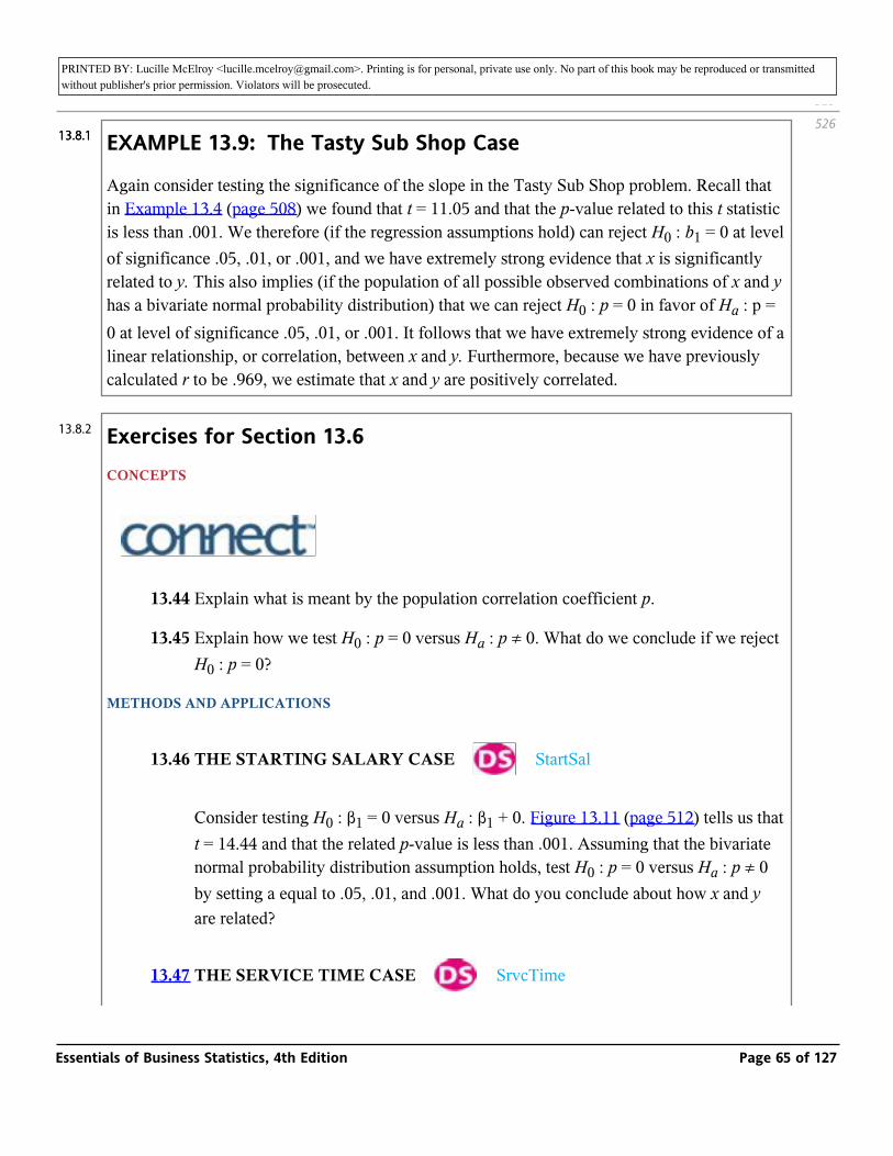
PRINTED BY: Lucille McElroy <[email protected]>. Printing is for personal, private use only. No part of this book may be reproduced or transmitted without publisher's prior permission. Violators will be prosecuted.discussed in Bowerman, O’Connell, and Murphree (2011).
EXAMPLE 13.9: The Tasty Sub Shop Case
Again consider testing the significance of the slope in the Tasty Sub Shop problem. Recall that in Example 13.4 (page 508) we found that t = 11.05 and that the p-value related to this t statistic is less than .001. We therefore (if the regression assumptions hold) can reject H0 : b1 = 0 at level of significance .05, .01, or .001, and we have extremely strong evidence that x is significantly related to y. This also implies (if the population of all possible observed combinations of x and y has a bivariate normal probability distribution) that we can reject H0 : p = 0 in favor of Ha : p = 0 at level of significance .05, .01, or .001. It follows that we have extremely strong evidence of a linear relationship, or correlation, between x and y. Furthermore, because we have previously calculated r to be .969, we estimate that x and y are positively correlated.
Exercises for Section 13.6CONCEPTS
_
13.44 Explain what is meant by the population correlation coefficient p.
13.45 Explain how we test H0 : p = 0 versus Ha : p ≠ 0. What do we conclude if we reject H0 : p = 0?
METHODS AND APPLICATIONS
13.46 THE STARTING SALARY CASE _ StartSal
Consider testing H0 : β1 = 0 versus Ha : β1 + 0. Figure 13.11 (page 512) tells us that t = 14.44 and that the related p-value is less than .001. Assuming that the bivariate normal probability distribution assumption holds, test H0 : p = 0 versus Ha : p ≠ 0 by setting a equal to .05, .01, and .001. What do you conclude about how x and y are related?
13.47 THE SERVICE TIME CASE _ SrvcTime
525
52613.8.113.8.1
13.8.2
Essentials of Business Statistics, 4th Edition Page 65 of 127

PRINTED BY: Lucille McElroy <[email protected]>. Printing is for personal, private use only. No part of this book may be reproduced or transmitted without publisher's prior permission. Violators will be prosecuted.
THE SERVICE TIME CASE _ SrvcTime
Consider testing H0 : β1 = 0 versus Ha : β1 ≠ 0. Figure 13.12 (page 512) tells us that t = 30.5802 and that the related p-value is less than .001. Assuming that the bivariate normal probability distribution assumption holds, test H0 : p = 0 versus Ha : p ≠ 0 by setting a equal to .05, .01, and .001. What do you conclude about how x and y are related?
13.7: An F Test for the Model
_ Test the significance of a simple linear regression model by using an F test.
In this section we discuss an F test that can be used to test the significance of the regression relationship between x and y. Sometimes people refer to this as testing the significance of the simple linear regression model. For simple linear regression, this test is another way to test the null hypothesis H0 : β1 = 0 (the relationship between x and y is not significant) versus Ha : β1 ≠ 0 (the relationship between x and y is significant). If we can reject H0 at level of significance a, we often say that the simple linear regression model is significant at level of significance α.
An F Test for the Simple Linear Regression Model
Suppose that the regression assumptions hold, and define the overall F statistic to be
Also define the p -value related to F (model) to be the area underthe curve of the F distribution (having 1 numerator and n - 2 denominator degrees of freedom) to the right of F (model)—see Figure 13.20(b).
13.9
13.9.1
Essentials of Business Statistics, 4th Edition Page 66 of 127

PRINTED BY: Lucille McElroy <[email protected]>. Printing is for personal, private use only. No part of this book may be reproduced or transmitted without publisher's prior permission. Violators will be prosecuted.Figure 13.20(b).
FIGURE 13.20(a): The F Test Critical Value
FIGURE 13.20(b): The F Test p -Value
Essentials of Business Statistics, 4th Edition Page 67 of 127

PRINTED BY: Lucille McElroy <[email protected]>. Printing is for personal, private use only. No part of this book may be reproduced or transmitted without publisher's prior permission. Violators will be prosecuted.
We can reject H0 : β1 = 0 in favor of Ha : β1 ≠ 0 at level of significance a if either of the following equivalent conditions holds:
1 F (model) > Fα
2 p -value < α
Here the point Fα is based on 1 numerator and n - 2 denominator degrees of freedom.
The first condition in the box says we should reject H0 : µ1 = 0 (and conclude that the relationship between x and y is significant) when F (model) is large. This is intuitive because a large overall F statistic would be obtained when the explained variation is large compared to the unexplained variation. This would occur if x is significantly related to y, which would imply that the slope β1 is not equal to 0. Figure 13.20(a) illustrates that we reject H0 when F (model) is greater than Fα. As can be seen in Figure 13.20(b), when F (model) is large, the related p-value is small. When the p -value is small enough [resulting from an F (model) statistic that is large enough], we reject H0. Figure 13.20(b) illustrates that the second condition in the box (p -value < a) is an equivalent way to carry out this test.
EXAMPLE 13.10: The Tasty Sub Shop Case _
Consider the Tasty Sub Shop problem and the following partial MINITAB output of the simple linear regression analysis relating yearly revenue y to population size x:
Looking at this output, we see that the explained variation is 465,316 and the unexplained variation is 30,460. It follows that
526
527
13.9.2
13.9.2
Essentials of Business Statistics, 4th Edition Page 68 of 127
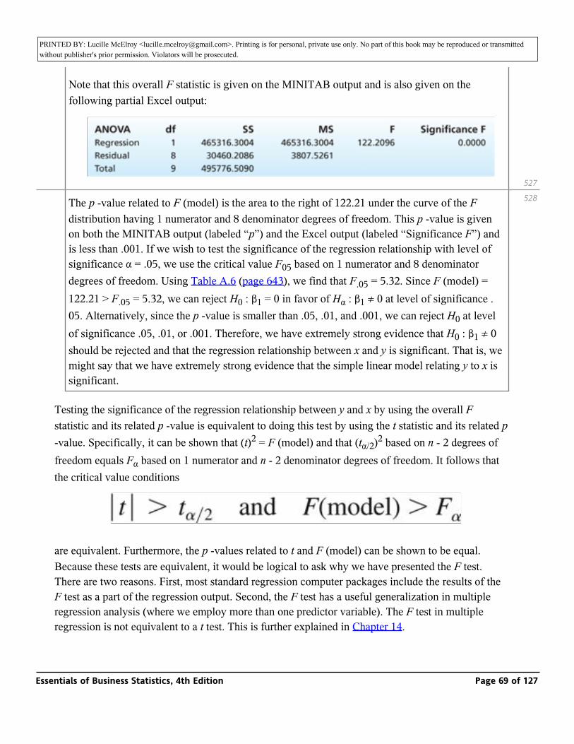
PRINTED BY: Lucille McElroy <[email protected]>. Printing is for personal, private use only. No part of this book may be reproduced or transmitted without publisher's prior permission. Violators will be prosecuted.
Note that this overall F statistic is given on the MINITAB output and is also given on the following partial Excel output:
The p -value related to F (model) is the area to the right of 122.21 under the curve of the F distribution having 1 numerator and 8 denominator degrees of freedom. This p -value is given on both the MINITAB output (labeled “p”) and the Excel output (labeled “Significance F”) and is less than .001. If we wish to test the significance of the regression relationship with level of significance α = .05, we use the critical value F05 based on 1 numerator and 8 denominator degrees of freedom. Using Table A.6 (page 643), we find that F.05 = 5.32. Since F (model) = 122.21 > F.05 = 5.32, we can reject H0 : β1 = 0 in favor of Hα : β1 ≠ 0 at level of significance .05. Alternatively, since the p -value is smaller than .05, .01, and .001, we can reject H0 at level of significance .05, .01, or .001. Therefore, we have extremely strong evidence that H0 : β1 ≠ 0 should be rejected and that the regression relationship between x and y is significant. That is, we might say that we have extremely strong evidence that the simple linear model relating y to x is significant.
Testing the significance of the regression relationship between y and x by using the overall F statistic and its related p -value is equivalent to doing this test by using the t statistic and its related p -value. Specifically, it can be shown that (t)2 = F (model) and that (tα/2)2 based on n - 2 degrees of freedom equals Fα based on 1 numerator and n - 2 denominator degrees of freedom. It follows that the critical value conditions
are equivalent. Furthermore, the p -values related to t and F (model) can be shown to be equal. Because these tests are equivalent, it would be logical to ask why we have presented the F test. There are two reasons. First, most standard regression computer packages include the results of the F test as a part of the regression output. Second, the F test has a useful generalization in multiple regression analysis (where we employ more than one predictor variable). The F test in multiple regression is not equivalent to a t test. This is further explained in Chapter 14.
527
528
Essentials of Business Statistics, 4th Edition Page 69 of 127

PRINTED BY: Lucille McElroy <[email protected]>. Printing is for personal, private use only. No part of this book may be reproduced or transmitted without publisher's prior permission. Violators will be prosecuted.regression is not equivalent to a t test. This is further explained in Chapter 14.
Exercises for Section 13.7CONCEPTS
_
13.48 What are the null and alternative hypotheses for the F test in simple linear regression?
13.49 The F test in simple linear regression is equivalent to what other test?
METHODS AND APPLICATIONS
In Exercises 13.50 through 13.55, we give MINITAB and Excel outputs of simple linear regression analyses of the data sets related to six previously discussed case studies. Using the appropriate computer output,
a Use the explained variation and the unexplained variation as given on the computer output to calculate (within rounding) the F (model) statistic.
b Utilize the F (model) statistic and the appropriate critical value to test H0 : β1 = 0 versus Hα : α1 ≠ 0 by setting a equal to .05. What do you conclude about the regression relationship between y and x?
c Utilize the F (model) statistic and the appropriate critical value to test H0 : β1 = 0 versus Hα : β1 ≠ 0 by setting a equal to .01. What do you conclude about the regression relationship between y and x?
d Find the p -value related to F (model) on the computer output and report its value. Using the p -value, test the significance of the regression model at the .10, .05, .01, and .001 levels of significance. What do you conclude?
e Show that the F (model) statistic is (within rounding) the square of the t statistic for testing H0 : β1 = 0 versus Hα : b1 ≠ 0. Also, show that the F.05 critical value is the square of the t025 critical value.
13.9.3
Essentials of Business Statistics, 4th Edition Page 70 of 127
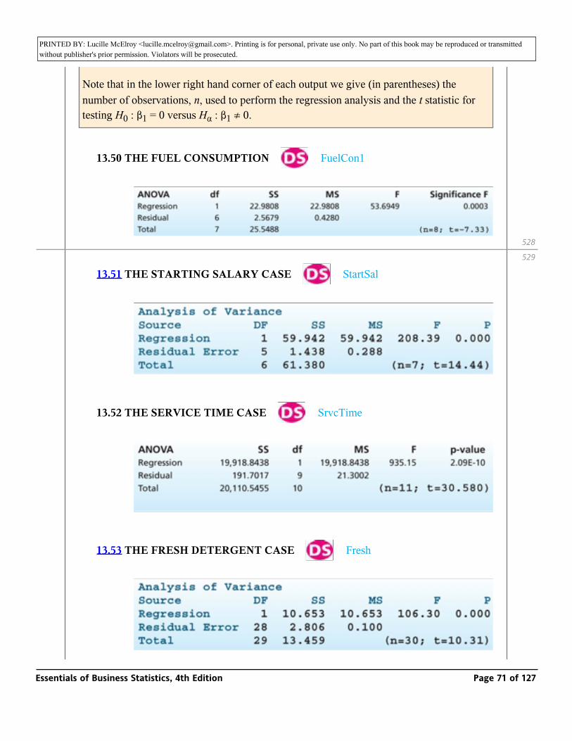
PRINTED BY: Lucille McElroy <[email protected]>. Printing is for personal, private use only. No part of this book may be reproduced or transmitted without publisher's prior permission. Violators will be prosecuted.square of the t025 critical value.
Note that in the lower right hand corner of each output we give (in parentheses) the number of observations, n, used to perform the regression analysis and the t statistic for testing H0 : β1 = 0 versus Hα : β1 ≠ 0.
13.50 THE FUEL CONSUMPTION _ FuelCon1
13.51 THE STARTING SALARY CASE _ StartSal
13.52 THE SERVICE TIME CASE _ SrvcTime
13.53 THE FRESH DETERGENT CASE _ Fresh
528
529
Essentials of Business Statistics, 4th Edition Page 71 of 127

PRINTED BY: Lucille McElroy <[email protected]>. Printing is for personal, private use only. No part of this book may be reproduced or transmitted without publisher's prior permission. Violators will be prosecuted.
13.54 THE DIRECT LABOR COST CASE _ DirLab
13.55 THE REAL ESTATE SALES PRICE CASE _ RealEst
13.8: The QHIC Case
Quality Home Improvement Center (QHIC) operates five stores in a large metropolitan area. The marketing department at QHIC wishes to study the relationship between x, home value (in thousands of dollars), and y, yearly expenditure on home upkeep (in dollars). A random sample of 40 homeowners is taken and asked to estimate their expenditures during the previous year on the types of home upkeep products and services offered by QHIC. Public records of the county auditor are used to obtain the previous year’s assessed values of the homeowner’s homes. The resulting x and y values, as well as a scatter plot of these values, are given in Figure 13.21. The Excel output included in this figure tells us that the least squares point estimates of the y -intercept β0 and the slope β1 are b0 = -348.3921 and b1 = 7.2583. The p -value associated with β1 i implies there is a significant linear relationship between x and y. In addition, because β1 = 7.2583, we estimate that mean yearly upkeep expenditure increases by $7.26 for each additional $1,000 increase in home value. Consider a home worth $220,000, and note that x0 = 220 is in the range of previously observed values of x : 48.9 to 286.18. It follows that is the point estimate of the mean yearly upkeep expenditure for all homes worth $220,000 and
1...
Essentials of Business Statistics, 4th Edition Page 72 of 127

PRINTED BY: Lucille McElroy <[email protected]>. Printing is for personal, private use only. No part of this book may be reproduced or transmitted without publisher's prior permission. Violators will be prosecuted.expenditure for all homes worth $220,000 and
FIGURE 13.21: The QHIC Upkeep Expenditure Data, Scatterplot,
and Excel Output _ QHIC
Essentials of Business Statistics, 4th Edition Page 73 of 127

PRINTED BY: Lucille McElroy <[email protected]>. Printing is for personal, private use only. No part of this book may be reproduced or transmitted without publisher's prior permission. Violators will be prosecuted.
529Essentials of Business Statistics, 4th Edition Page 74 of 127

PRINTED BY: Lucille McElroy <[email protected]>. Printing is for personal, private use only. No part of this book may be reproduced or transmitted without publisher's prior permission. Violators will be prosecuted.
is the point prediction of a yearly upkeep expenditure for an individual home worth $220,000.
_
The marketing department at QHIC wishes to determine which homes should be sent advertising brochures promoting QHIC’s products and services. If the marketing department has decided to send an advertising brochure to any home that has a predicted yearly upkeep expenditure of at least $500, then a home worth $220,000 would be sent an advertising brochure. This is because the predicted yearly upkeep expenditure for such a home is (as calculated above) $1,248.43. Other homes can be evaluated in a similar fashion.
13.9: Residual Analysis
_ Use residual analysis to check the assumptions of simple linear regression.
In this section we explain how to check the validity of the regression assumptions. The required checks are carried out by analyzing the regression residuals. The residuals are defined as follows:
For any particular observed value of y, the corresponding residual is
e = y - ŷ = (observed value of y - predicted value of y)
where the predicted value of y is calculated using the least squares prediction equation
The linear regression model y = β0 + β1 x + ε implies that the error term ε is given by the equation ε = y - (β0 + β1 x). Since ŷ in the previous box is clearly the point estimate of β0 + β1 x, we see that the residual ε = y - ŷ is the point estimate of the error term ε. If the regression assumptions are valid, then, for any given value of the independent variable, the population of potential error term values will be normally distributed with mean 0 and variance σ2 (see the regression assumptions in Section
529
531
1...
Essentials of Business Statistics, 4th Edition Page 75 of 127

PRINTED BY: Lucille McElroy <[email protected]>. Printing is for personal, private use only. No part of this book may be reproduced or transmitted without publisher's prior permission. Violators will be prosecuted.then, for any given value of the independent variable, the population of potential error term values
will be normally distributed with mean 0 and variance σ2 (see the regression assumptions in Section 13.2 on page 504). Furthermore, the different error terms will be statistically independent. Because the residuals provide point estimates of the error terms, it follows that
If the regression assumptions hold, the residuals should look like they have been randomly and independently selected from normally distributed populations having mean 0 and variance σ2.
In any real regression problem, the regression assumptions will not hold exactly. In fact, it is important to point out that mild departures from the regression assumptions do not seriously hinder our ability to use a regression model to make statistical inferences. Therefore, we are looking for pronounced, rather than subtle, departures from the regression assumptions. Because of this, we will require that the residuals only approximately fit the description just given.
Residual plots
One useful way to analyze residuals is to plot them versus various criteria. The resulting plots are called residual plots. To construct a residual plot, we compute the residual for each observed y value. The calculated residuals are then plotted versus some criterion. To validate the regression assumptions, we make residual plots against (1) values of the independent variable x; (2) values of y, the predicted value of the dependent variable; and (3) the time order in which the data have been observed (if the regression data are time series data).
We next look at an example of constructing residual plots. Then we explain how to use these plots to check the regression assumptions.
EXAMPLE 13.11: The QHIC Case _
Figure 13.21 gives the QHIC upkeep expenditure data and a scatterplot of the data. If we use a simple linear regression model to describe the QHIC data, we find that the least squares point estimates of β0 and β1 are b0 = -348.3921 and b1 = 7.2583. The Excel add-in (MegaStat) output in Figure 13.22(a) presents the predicted home upkeep expenditures and residuals that are given by the simple linear regression model. Here each residual is computed as
531
532
13.1...
13.11.1.1
13.11.1.1
Essentials of Business Statistics, 4th Edition Page 76 of 127

PRINTED BY: Lucille McElroy <[email protected]>. Printing is for personal, private use only. No part of this book may be reproduced or transmitted without publisher's prior permission. Violators will be prosecuted.are given by the simple linear regression model. Here each residual is computed as
FIGURE 13.22: Residuals and Residual Plots for the QHIC Simple Linear Regression Model
For instance, for the first observation (home) when y = 1,412.08 and x = 237.00 (see Figure 13.21), the residual is
The MINITAB output in Figure 13.22(b) and (c) gives plots of the residuals for the QHIC simple linear regression model against values of x and ŷ. To understand how these plots are constructed, recall that for the first observation (home) y = 1,412.08, x = 237.00, ŷ = 1,371.816, and the residual is 40.264. It follows that the point plotted in Figure 13.22(b)
Essentials of Business Statistics, 4th Edition Page 77 of 127

PRINTED BY: Lucille McElroy <[email protected]>. Printing is for personal, private use only. No part of this book may be reproduced or transmitted without publisher's prior permission. Violators will be prosecuted.constructed, recall that for the first observation (home) y = 1,412.08, x = 237.00, ŷ =
1,371.816, and the residual is 40.264. It follows that the point plotted in Figure 13.22(b) corresponding to the first observation has a horizontal axis coordinate of the x value 237.00 and a vertical axis coordinate of the residual 40.264. It also follows that the point plotted in Figure 13.22(c) corresponding to the first observation has a horizontal axis coordinate of the ŷ value 1,371.816, and a vertical axis coordinate of the residual 40.264. Finally, note that the QHIC data are cross-sectional data, not time series data. Therefore, we cannot make a residual plot versus time.
The constant variance assumption
To check the validity of the constant variance assumption, we examine plots of the residuals against values of x, ŷ, and time (if the regression data are time series data). When we look at these plots, the pattern of the residuals’ fluctuation around 0 tells us about the validity of the constant variance assumption. A residual plot that “fans out” [as in Figure 13.23(a)] suggests that the error terms are becoming more spread out as the horizontal plot value increases and that the constant variance assumption is violated. Here we would say that an increasing error variance exists. A residual plot that “funnels in” [as in Figure 13.23(b)] suggests that the spread of the error terms is decreasing as the horizontal plot value increases and that again the constant variance assumption is violated. In this case we would say that a decreasing error variance exists. A residual plot with a “horizontal band appearance” [as in Figure 13.23(c)] suggests that the spread of the error terms around 0 is not changing much as the horizontal plot value increases. Such a plot tells us that the constant variance assumption (approximately) holds.
FIGURE 13.23: Residual Plots and the Constant Variance Assumption
532
53313.1...
Essentials of Business Statistics, 4th Edition Page 78 of 127

PRINTED BY: Lucille McElroy <[email protected]>. Printing is for personal, private use only. No part of this book may be reproduced or transmitted without publisher's prior permission. Violators will be prosecuted.
As an example, consider the QHIC case and the residual plot in Figure 13.22(b). This plot appears to fan out as x increases, indicating that the spread of the error terms is increasing as x increases. That is, an increasing error variance exists. This is equivalent to saying that the variance of the population of potential yearly upkeep expenditures for houses worth x (thousand dollars) appears to increase as x increases. The reason is that the model y = β0 + β1 x + ε says that the variation of y is the same as the variation of e. For example, the variance of the population of potential yearly upkeep expenditures for houses worth $200,000 would be larger than the variance of the population of potential yearly upkeep expenditures for houses worth $100,000. Increasing variance makes some intuitive sense because people with more expensive homes generally have more discretionary income. These people can choose to spend either a substantial amount or a much smaller amount on home upkeep, thus causing a relatively large variation in upkeep expenditures.
Another residual plot showing the increasing error variance in the QHIC case is Figure 13.22(c). This plot tells us that the residuals appear to fan out as ŷ (predicted y) increases, which is logical because ŷ is an increasing function of x. Also, note that the scatter plot of y versus x in Figure 13.21 shows the increasing error variance—the y values appear to fan out as x increases. In fact, one might ask why we need to consider residual plots when we can simply look at scatter plots of y versus x. One answer is that, in general, because of possible differences in scaling between residual plots and scatter plots of y versus x, one of these types of plots might be more informative in a particular situation. Therefore, we should always consider both types of plots.
When the constant variance assumption is violated, we cannot use the formulas of this chapter to make statistical inferences. Later in this section we discuss how we can make statistical inferences when a nonconstant error variance exists.
The assumption of correct functional form
If the functional form of a regression model is incorrect, the residual plots constructed by using the model often display a pattern suggesting the form of a more appropriate model. For instance, if we use a simple linear regression model when the true relationship between y and x is curved, the residual plot will have a curved appearance. For example, the scatter plot of upkeep expenditure, y, versus home value, x, in Figure 13.21 (page 530) has either a straight-line or slightly curved appearance. We used a simple linear regression model to describe the relationship between y and x, but note that there is a “dip,” or slightly curved appearance, in the upper left portion of each residual plot in Figure 13.22. Therefore, both the scatter plot and residual plots indicate that there might be a slightly curved relationship between y and x. Later in this section we discuss one way to model curved relationships.
533
53413.1...
Essentials of Business Statistics, 4th Edition Page 79 of 127

PRINTED BY: Lucille McElroy <[email protected]>. Printing is for personal, private use only. No part of this book may be reproduced or transmitted without publisher's prior permission. Violators will be prosecuted.to model curved relationships.
The normality assumption
If the normality assumption holds, a histogram and/or stem-and-leaf display of the residuals should look reasonably bell-shaped and reasonably symmetric about 0. Figure 13.24(a) gives the MINITAB output of a stem-and-leaf display of the residuals from the simple linear regression model describing the QHIC data. The stem-and-leaf display looks fairly bell-shaped and symmetric about 0. However, the tails of the display look somewhat long and “heavy” or “thick,” indicating a possible violation of the normality assumption.
FIGURE 13.24: Stem-and-Leaf Display and Normal Plots of the Residuals from the Simple Linear Regression Model Describing the QHIC Data
Another way to check the normality assumption is to construct a normal plot of the residuals. To make a normal plot, we first arrange the residuals in order from smallest to largest. Letting the ordered residuals be denoted as e(1), e(2),. . ., e(n) we denote the i th residual in the ordered listing as e(i). We plot e(i) on the vertical axis against a point called z(i) on the horizontal axis. Here z{i) is defined to be the point on the horizontal axis under the standard normal curve so that the area
13.1...
Essentials of Business Statistics, 4th Edition Page 80 of 127

PRINTED BY: Lucille McElroy <[email protected]>. Printing is for personal, private use only. No part of this book may be reproduced or transmitted without publisher's prior permission. Violators will be prosecuted.as e(i). We plot e(i) on the vertical axis against a point called z(i) on the horizontal axis. Here z{i) is
defined to be the point on the horizontal axis under the standard normal curve so that the area under this curve to the left of z{i) is (3i - 1)/(3n + 1). For example, recall in the QHIC case that there are n = 40 residuals given in Figure 13.22(a). It follows that, when i = 1, then
Therefore, z(1) is the normal point having an area of .0165 under the standard normal curve to its left. Thus, as illustrated in Figure 13.24(b), z(1) equals - 2.13. Because the smallest residual in Figure 13.22(a) is -289.044, the first point plotted is e(1) = -289.044 on the vertical scale versus Z (1) = -2.13 on the horizontal scale. When i = 2, it can be verified that (3i - 1)/(3n + 1) equals .0413 and thus that z(2) = -1.74. Therefore, because the second-smallest residual in Figure 13.24(a) is -259.958, the second point plotted is e(2) =-259.958 on the vertical scale versus z(2) =-1.74 on the horizontal scale. This process is continued until the entire normal plot is constructed. The Excel add-in (MegaStat) output of this plot is given in Figure 13.24(c).
An equivalent plot is shown in Figure 13.24(d), which is a MINITAB output. In this figure, we plot the percentage p(i) of the area under the standard normal curve to the left of z(i) on the vertical axis. Thus, the first point plotted in this normal plot is e(V) = -289.044 on the horizontal scale versus p{l) = (.0165)(100) = 1.65 on the vertical scale, and the second point plotted is e (2) = -259.958 on the horizontal scale versus p{1) = (.0413)(100) = 4.13 on the vertical scale. It is important to note that the scale on the vertical axis does not have the usual spacing between the percentages. The spacing reflects the distance between the z -scores that correspond to the percentages in the standard normal distribution. Hence, if we wished to create the plot in Figure 13.24(d) by hand, we would need special graphing paper with this vertical scale.
It can be proven that, if the normality assumption holds, then the expected value of the i th ordered residual e(i) is proportional to z(i). Therefore, a plot of the e(i) values on the horizontal scale versus the z(i) values on the vertical scale (or equivalently, the e(i) values on the horizontal scale versus the p(i) values on the vertical scale) should have a straight-line appearance. That is, if the normality assumption holds, then the normal plot should have a straight-line appearance. A normal plot that does not look like a straight line (admittedly, a subjective decision) indicates that the normality assumption is violated. Since the normal plots in Figure 13.24 have some curvature (particularly in the upper right portion), there is a possible violation of the normality assumption.
It is important to realize that violations of the constant variance and correct functional form assumptions can often cause a histogram and/or stem-and-leaf display of the residuals to look nonnormal and can cause the normal plot to have a curved appearance. Because of this, it is
534
535
Essentials of Business Statistics, 4th Edition Page 81 of 127

PRINTED BY: Lucille McElroy <[email protected]>. Printing is for personal, private use only. No part of this book may be reproduced or transmitted without publisher's prior permission. Violators will be prosecuted.assumptions can often cause a histogram and/or stem-and-leaf display of the residuals to look
nonnormal and can cause the normal plot to have a curved appearance. Because of this, it is usually a good idea to use residual plots to check for nonconstant variance and incorrect functional form before making any final conclusions about the normality assumption. Later in this section we discuss a procedure that sometimes remedies simultaneous violations of the constant variance, correct functional form, and normality assumptions.
The independence assumption
The independence assumption is most likely to be violated when the regression data are time series data—that is, data that have been collected in a time sequence. For such data the time-ordered error terms can be autocorrelated. Intuitively, we say that error terms occurring over time have positive autocorrelation if a positive error term in time period i tends to produce, or be followed by, another positive error term in time period i + k (some later time period) and if a negative error term in time period i tends to produce, or be followed by, another negative error term in time period i + k. In other words, positive autocorrelation exists when positive error terms tend to be followed over time by positive error terms and when negative error terms tend to be followed over time by negative error terms. Positive autocorrelation in the error terms is depicted in Figure 13.25(a), which illustrates that positive autocorrelation can produce a cyclical error term pattern over time. The simple linear regression model implies that a positive error term produces a greater-than-average value of y and a negative error term produces a smaller-than-average value of y. It follows that positive autocorrelation in the error terms means that greater-than-average values of y tend to be followed by greater-than-average values of y, and smaller-than-average values of y tend to be followed by smaller-than-average values of y. An example of positive autocorrelation could hypothetically be provided by a simple linear regression model relating demand for a product to advertising expenditure. Here we assume that the data are time series data observed over a number of consecutive sales periods. One of the factors included in the error term of the simple linear regression model is competitors’ advertising expenditure for their similar products. If, for the moment, we assume that competitors’ advertising expenditure significantly affects the demand for the product, then a higher-than-average competitors’ advertising expenditure probably causes demand for the product to be lower than average and hence probably causes a negative error term. On the other hand, a lower-than-average competitors’ advertising expenditure probably causes the demand for the product to be higher than average and hence probably causes a positive error term. If, then, competitors tend to spend money on advertising in a cyclical fashion—spending large amounts for several consecutive sales periods (during an advertising campaign) and then spending lesser amounts for several consecutive sales periods—a negative error term in one sales period will tend to be followed by a negative error term in the next sales period, and a positive error term in one sales period will tend to be followed by a positive error term in the next sales period. In this case the error terms would display positive autocorrelation, and thus these error terms would not be statistically independent.
535
536
13.1...
Essentials of Business Statistics, 4th Edition Page 82 of 127

PRINTED BY: Lucille McElroy <[email protected]>. Printing is for personal, private use only. No part of this book may be reproduced or transmitted without publisher's prior permission. Violators will be prosecuted.display positive autocorrelation, and thus these error terms would not be statistically independent.
FIGURE 13.25: Positive and Negative Autocorrelation
Intuitively, error terms occurring over time have negative autocorrelation if a positive error term in time period i tends to produce, or be followed by, a negative error term in time period i + k and if a negative error term in time period i tends to produce, or be followed by, a positive error term in time period i + k. In other words, negative autocorrelation exists when positive error terms tend to be followed over time by negative error terms and negative error terms tend to be followed over time by positive error terms. An example of negative autocorrelation in the error terms is depicted in Figure 13.25(b), which illustrates that negative autocorrelation in the error terms can produce an alternating pattern over time. It follows that negative autocorrelation in the error terms means that greater-than-average values of y tend to be followed by smaller-than-average values of y and smaller-than-average values of y tend to be followed by greater-than-average values of y. An example of negative autocorrelation might be provided by a retailer’s weekly stock orders. Here a larger-than-average stock order one week might result in an oversupply and hence a smaller-than-average order the next week.
The independence assumption basically says that the time-ordered error terms display no positive or negative autocorrelation. This says that the error terms occur in a random pattern over time. Such a random pattern would imply that the error terms (and their corresponding y values) are statistically independent.
Because the residuals are point estimates of the error terms, a residual plot versus time is used to check the independence assumption. If a residual plot versus the data’s time sequence has a cyclical appearance, the error terms are positively autocorrelated, and the independence assumption is violated. If a plot of the time-ordered residuals has an alternating pattern, the error terms are negatively autocorrelated, and again the independence assumption is violated. However, if a plot of the time-ordered residuals displays a random pattern, the error terms have little or no autocorrelation. In such a case, it is reasonable to conclude that the independence assumption holds.
536
537
Essentials of Business Statistics, 4th Edition Page 83 of 127

PRINTED BY: Lucille McElroy <[email protected]>. Printing is for personal, private use only. No part of this book may be reproduced or transmitted without publisher's prior permission. Violators will be prosecuted.holds.
EXAMPLE 13.12
Figure 13.26(a) presents data concerning weekly sales at Pages Bookstore (Sales), Pages weekly advertising expenditure (Adver), and the weekly advertising expenditure of Pages main competitor (Compadv). Here the sales values are expressed in thousands of dollars, and the advertising expenditure values are expressed in hundreds of dollars. Figure 13.26(a) also gives the MINITAB output of the residuals that are obtained when a simple linear regression analysis is performed relating Pages sales to Pages advertising expenditure. These residuals are plotted versus time in Figure 13.26(b). We see that the residual plot has a cyclical pattern. This tells us that the error terms for the model are positively autocorrelated and the independence assumption is violated. Furthermore, there tend to be positive residuals when the competitor’s advertising expenditure is lower (in weeks 1 through 8 and weeks 14, 15, and 16) and negative residuals when the competitor’s advertising expenditure is higher (in weeks 9 through 13). Therefore, the competitor’s advertising expenditure seems to be causing the positive autocorrelation.
FIGURE 13.26: Pages Bookstore Sales and Advertising Data, and Residual Analysis
537
13.11.5.1
Essentials of Business Statistics, 4th Edition Page 84 of 127

PRINTED BY: Lucille McElroy <[email protected]>. Printing is for personal, private use only. No part of this book may be reproduced or transmitted without publisher's prior permission. Violators will be prosecuted.
To conclude this example, note that the simple linear regression model relating Pages sales to Pages advertising expenditure has a standard error, s, of 5.038. The residual plot in Figure 13.26(b) includes grid lines that are placed one and two standard errors above and below the residual mean of 0. Such grid lines help us to better diagnose potential violations of the regression assumptions.
When the independence assumption is violated, various remedies can be employed. One approach is to identify which independent variable left in the error term (for example, competitors’ advertising expenditure) is causing the error terms to be autocorrelated. We can then remove this independent variable from the error term and insert it directly into the regression model, forming a multiple regression model. (Multiple regression models are discussed in Chapter 14.)
The Durbin–Watson test
One type of positive or negative autocorrelation is called first-order autocorrelation. It says that εt, the error term in time period t, is related to εt -1, the error term in time period t - 1. To check for first-order autocorrelation, we can use the Durbin–Watson statistic
where e1, e2, ..., en are the time-ordered residuals.
Intuitively, small values of d lead us to conclude that there is positive autocorrelation. This is because, if d is small, the differences (et - et -1) are small. This indicates that the adjacent residuals et and et -1 are of the same magnitude, which in turn says that the adjacent error terms et and et -1 are positively correlated. Consider testing the null hypothesis H0 that the error terms are not autocorrelated versus the alternative hypothesis Hα that the error terms are positively autocorrelated. Durbin and Watson have shown that there are points (denoted dL α and dU α) such that, if a is the probability of a Type I error, then
537
538
13.1...
Essentials of Business Statistics, 4th Edition Page 85 of 127
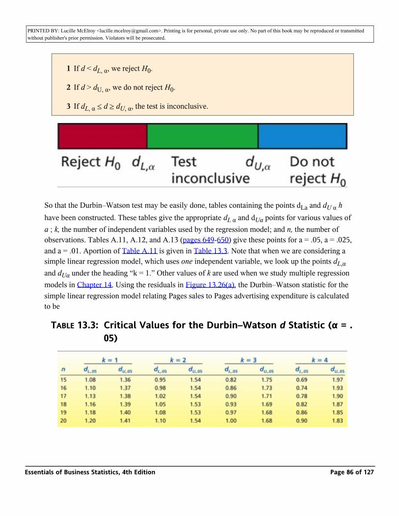
PRINTED BY: Lucille McElroy <[email protected]>. Printing is for personal, private use only. No part of this book may be reproduced or transmitted without publisher's prior permission. Violators will be prosecuted.that, if a is the probability of a Type I error, then
1 If d < dL, α, we reject H0.
2 If d > dU, α, we do not reject H0.
3 If dL, α ≤ d ≥ dU, α, the test is inconclusive.
So that the Durbin–Watson test may be easily done, tables containing the points dLa and dU α h have been constructed. These tables give the appropriate dL α and dUα points for various values of a ; k, the number of independent variables used by the regression model; and n, the number of observations. Tables A.11, A.12, and A.13 (pages 649-650) give these points for a = .05, a = .025, and a = .01. Aportion of Table A.11 is given in Table 13.3. Note that when we are considering a simple linear regression model, which uses one independent variable, we look up the points dL,α and dUα under the heading “k = 1.” Other values of k are used when we study multiple regression models in Chapter 14. Using the residuals in Figure 13.26(a), the Durbin–Watson statistic for the simple linear regression model relating Pages sales to Pages advertising expenditure is calculated to be
TABLE 13.3: Critical Values for the Durbin–Watson d Statistic (α = .05)
Essentials of Business Statistics, 4th Edition Page 86 of 127
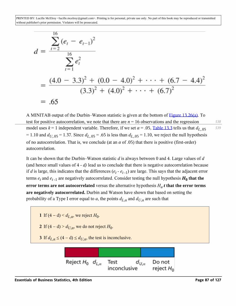
PRINTED BY: Lucille McElroy <[email protected]>. Printing is for personal, private use only. No part of this book may be reproduced or transmitted without publisher's prior permission. Violators will be prosecuted.
A MINITAB output of the Durbin–Watson statistic is given at the bottom of Figure 13.26(a). To test for positive autocorrelation, we note that there are n = 16 observations and the regression model uses k = 1 independent variable. Therefore, if we set α = .05, Table 13.3 tells us that dL,.05 = 1.10 and dU,.05 = 1.37. Since dL,.05 = .65 is less than dL,.05 = 1.10, we reject the null hypothesis of no autocorrelation. That is, we conclude (at an α of .05) that there is positive (first-order) autocorrelation.
It can be shown that the Durbin–Watson statistic d is always between 0 and 4. Large values of d (and hence small values of 4 - d) lead us to conclude that there is negative autocorrelation because if d is large, this indicates that the differences (et - et -1) are large. This says that the adjacent error terms et and et -1 are negatively autocorrelated. Consider testing the null hypothesis H0 that the error terms are not autocorrelated versus the alternative hypothesis Ha t that the error terms are negatively autocorrelated. Durbin and Watson have shown that based on setting the probability of a Type I error equal to a, the points dL,α and dU,α are such that
1 If (4 − d) < dL,α, we reject H0.
2 If (4 − d) > dU,α, we do not reject H0.
3 If dL,α ≤ (4 − d) ≤ dU,α, the test is inconclusive.
538
539
Essentials of Business Statistics, 4th Edition Page 87 of 127
PRINTED BY: Lucille McElroy <[email protected]>. Printing is for personal, private use only. No part of this book may be reproduced or transmitted without publisher's prior permission. Violators will be prosecuted.
As an example, for the Pages sales simple linear regression model, we see that
Therefore, on the basis of setting a equal to .05, we do not reject the null hypothesis of no autocorrelation. That is, there is no evidence of negative (first-order) autocorrelation.
We can also use the Durbin–Watson statistic to test for positive or negative autocorrelation. Specifically, consider testing the null hypothesis H0 that the error terms are not autocorrelated versus the alternative hypothesis Ha that the error terms are positively or negatively autocorrelated. Durbin and Watson have shown that, based on setting the probability of a Type I error equal to a, we perform both the above described test for positive autocorrelation and the above described test for negative autocorrelation by using the critical values dL,.α/2 and dU,.α/2 for each test. If either test says to reject H0 then we reject H0. If both tests say to not reject H0, then we do not reject H0. Finally, if either test is inconclusive, then the overall test is inconclusive. For example, consider testing for positive or negative autocorrelation in the Pages sales model. If we set α equal to .05, then a/2 = .025, and we need to find the points dL,.025 and dU,.025 when n = 16 and k = 1. Looking up these points in Table A.12 (page 649), we find that dL,.025 = .98 and dU,.025 = 1.24. Since d = .65 is less than dL,.025 = .98, we reject the null hypothesis of no autocorrelation. That is, we conclude (at an a of .05) that there is first-order autocorrelation.
Although we have used the Pages sales model in these examples to demonstrate the Durbin–Watson tests for (1) positive autocorrelation, (2) negative autocorrelation, and (3) positive or negative autocorrelation, we must in practice choose one of these Durbin-Watson tests in a particular situation. Since positive autocorrelation is more common in real time series data than negative autocorrelation, the Durbin–Watson test for positive autocorrelation is used more often than the other two tests. Also, note that each Durbin–Watson test assumes that the population of all possible residuals at any time t has a normal distribution.
Transforming the dependent variable: A possible remedy for violations of the constant variance, correct functional form, and normality assumptions
In general, if a data or residual plot indicates that the error variance of a regression model increases as an independent variable or the predicted value of the dependent variable increases, then we can sometimes remedy the situation by transforming the dependent variable. One transformation that works well is to take each y value to a fractional power. As an example, we might use a transformation in which we take the square root (or one-half power) of each y value. Letting y* denote the value obtained when the transformation is applied to y, we would write the
539
540
13.1...
Essentials of Business Statistics, 4th Edition Page 88 of 127
PRINTED BY: Lucille McElroy <[email protected]>. Printing is for personal, private use only. No part of this book may be reproduced or transmitted without publisher's prior permission. Violators will be prosecuted.might use a transformation in which we take the square root (or one-half power) of each y value.
Letting y* denote the value obtained when the transformation is applied to y, we would write the square root transformation as
Another commonly used transformation is the quartic root transformation. Here we take each y value to the one-fourth power. That is,
If we consider a transformation that takes each y value to a fractional power (such as .5, .25, or the like), as the power approaches 0, the transformed value y* approaches the natural logarithm of y (commonly written ln y). In fact, we sometimes use the logarithmic transformation
which takes the natural logarithm of each y value. In general, when we take a fractional power (including the natural logarithm) of the dependent variable, the transformation not only tends to equalize the error variance but also tends to “straighten out” certain types of nonlinear data plots. Specifically, if a data plot indicates that the dependent variable is increasing at an increasing rate, then a fractional power transformation tends to straighten out the data plot. A fractional power transformation can also help to remedy a violation of the normality assumption. Because we cannot know which fractional power to use before we actually take the transformation, we recommend taking all of the square root, quartic root, and natural logarithm transformations and seeing which one best equalizes the error variance and (possibly) straightens out a nonlinear data plot.
EXAMPLE 13.13: The QHIC Case _
Consider the QHIC upkeep expenditures in Figure 13.21. In Figures 13.27, 13.28, and 13.29 we show the plots that result when we take the square root, quartic root, and natural logarithmic transformations of the upkeep expenditures and plot the transformed values versus the home values. The square root transformation seems to best equalize the error variance and straighten out the curved data plot in Figure 13.21. Note that the natural
13.11.7.1
13.11.7.1
Essentials of Business Statistics, 4th Edition Page 89 of 127
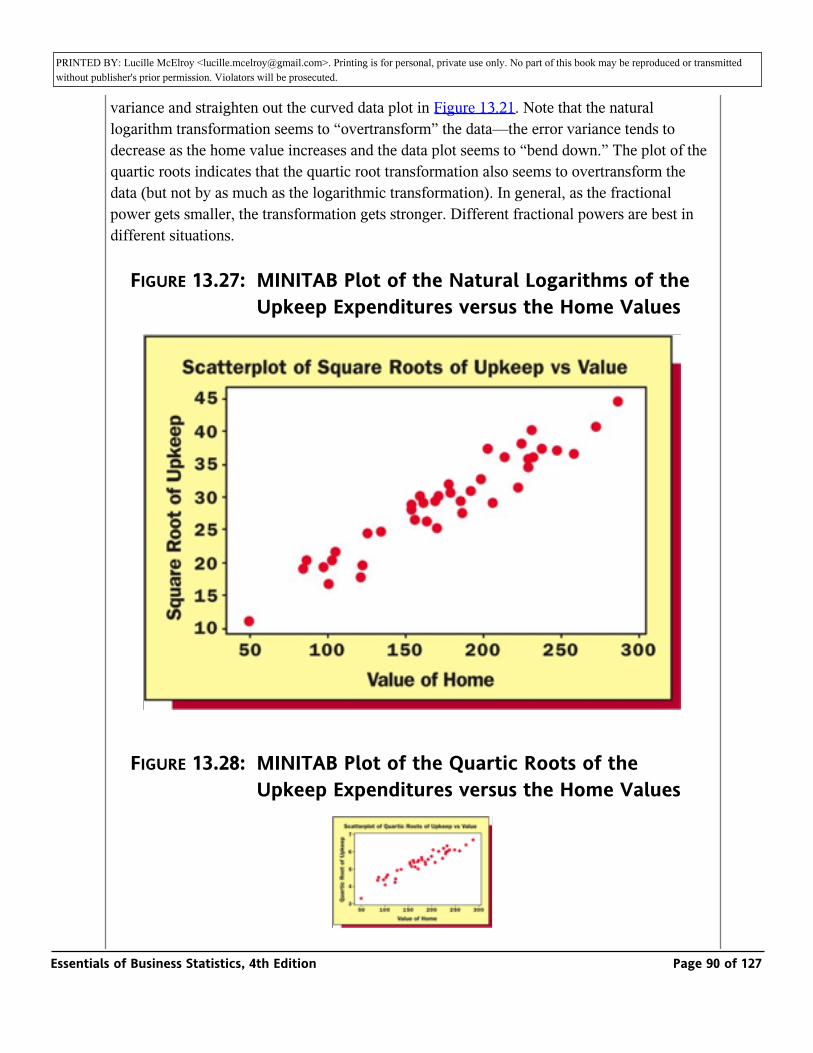
PRINTED BY: Lucille McElroy <[email protected]>. Printing is for personal, private use only. No part of this book may be reproduced or transmitted without publisher's prior permission. Violators will be prosecuted.versus the home values. The square root transformation seems to best equalize the error
variance and straighten out the curved data plot in Figure 13.21. Note that the natural logarithm transformation seems to “overtransform” the data—the error variance tends to decrease as the home value increases and the data plot seems to “bend down.” The plot of the quartic roots indicates that the quartic root transformation also seems to overtransform the data (but not by as much as the logarithmic transformation). In general, as the fractional power gets smaller, the transformation gets stronger. Different fractional powers are best in different situations.
FIGURE 13.27: MINITAB Plot of the Natural Logarithms of the Upkeep Expenditures versus the Home Values
FIGURE 13.28: MINITAB Plot of the Quartic Roots of the Upkeep Expenditures versus the Home Values
Essentials of Business Statistics, 4th Edition Page 90 of 127
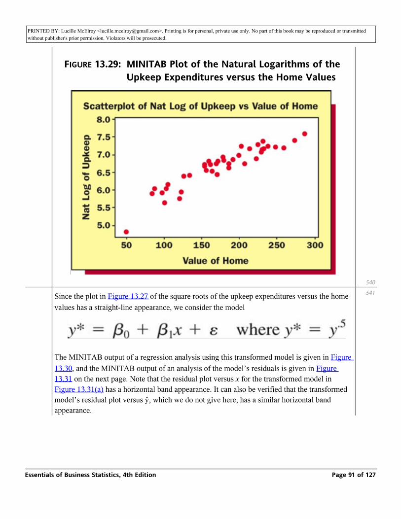
PRINTED BY: Lucille McElroy <[email protected]>. Printing is for personal, private use only. No part of this book may be reproduced or transmitted without publisher's prior permission. Violators will be prosecuted.
FIGURE 13.29: MINITAB Plot of the Natural Logarithms of the Upkeep Expenditures versus the Home Values
Since the plot in Figure 13.27 of the square roots of the upkeep expenditures versus the home values has a straight-line appearance, we consider the model
The MINITAB output of a regression analysis using this transformed model is given in Figure 13.30, and the MINITAB output of an analysis of the model’s residuals is given in Figure 13.31 on the next page. Note that the residual plot versus x for the transformed model in Figure 13.31(a) has a horizontal band appearance. It can also be verified that the transformed model’s residual plot versus ŷ, which we do not give here, has a similar horizontal band appearance.
540
541
Essentials of Business Statistics, 4th Edition Page 91 of 127

PRINTED BY: Lucille McElroy <[email protected]>. Printing is for personal, private use only. No part of this book may be reproduced or transmitted without publisher's prior permission. Violators will be prosecuted.appearance.
FIGURE 13.30: MINITAB Output of a Regression Analysis of the Upkeep Expenditure Data by Using the Model y * = β0 + β1 x + ε where y * = y 5
Therefore, we conclude that the constant variance and the correct functional form assumptions approximately hold for the transformed model. Next, note that the histogram of the transformed model’s residuals in Figure 13.31(b) looks reasonably bell-shaped and symmetric, and note that the normal plot of these residuals in Figure 13.31(c) looks straighter than the normal plots for the untransformed model (see Figure 13.24 on page 535). Therefore, we also conclude that the normality assumption approximately holds for the transformed model.
FIGURE 13.31: MINITAB Output of Residual Analysis for the Upkeep Expenditure Model y * = β0 + β1 x + ε
where y * = y 5
541
542
Essentials of Business Statistics, 4th Edition Page 92 of 127

PRINTED BY: Lucille McElroy <[email protected]>. Printing is for personal, private use only. No part of this book may be reproduced or transmitted without publisher's prior permission. Violators will be prosecuted.
Because the regression assumptions approximately hold for the transformed regression model, we can use this model to make statistical inferences. Consider a home worth $220,000. Using the least squares point estimates on the MINITAB output in Figure 13.30 on the previous page, it follows that a point prediction of y* for such a home is
_
This point prediction is given at the bottom of the MINITAB output, as is the 95 percent prediction interval for y*, which is [30.348, 39.954]. It follows that a point prediction of the upkeep expenditure for a home worth $220,000 is (35.151)2 = $1,235.59 and that a 95 percent prediction interval for this upkeep expenditure is [(30.348)2, (39.954)2 ] = [$921.00, $1596.32]. Suppose that QHIC wishes to send an advertising brochure to any home that has a predicted upkeep expenditure of at least $500. It follows that a home worth $220,000 would be sent an advertising brocedure. This is because the predicted yearly upkeep expenditure for such a home is (as just calculated) $1,235.59. Other homes can be evaluated in a similar fashion.
Exericses for Section 13.9CONCEPTS
_
13.56 In a regression analysis, what variables should the residuals be plotted against? What types of patterns in residual plots indicate violations of the regression assumptions?
542
54313.11.7.2
Essentials of Business Statistics, 4th Edition Page 93 of 127

PRINTED BY: Lucille McElroy <[email protected]>. Printing is for personal, private use only. No part of this book may be reproduced or transmitted without publisher's prior permission. Violators will be prosecuted.assumptions?
13.57 In regression analysis, how do we check the normality assumption?
13.58 What is one possible remedy for violations of the constant variance, correct functional form, and normality assumptions?
METHODS AND APPLICATIONS
13.59 THE FUEL CONSUMPTION CASE _ FuelConl
Figure 13.32(a) gives the Excel output of a plot of the residuals obtained by fitting a simple linear regression model to the fuel consumption data. Describe the appearance of this plot. Does the plot indicate any violations of the regression assumptions?
FIGURE 13.32: Residual Diagnostics for Exercises 13.59 and 13.60
13.60 THE FRESH DETERGENT CASE _ Fresh
Figure 13.32(b) gives the MINITAB output of residual diagnostics that are obtained when the simple linear regression model is fit to the Fresh detergent demand data. Interpret the diagnostics and determine if they indicate any violations of the regression assumptions.
Essentials of Business Statistics, 4th Edition Page 94 of 127
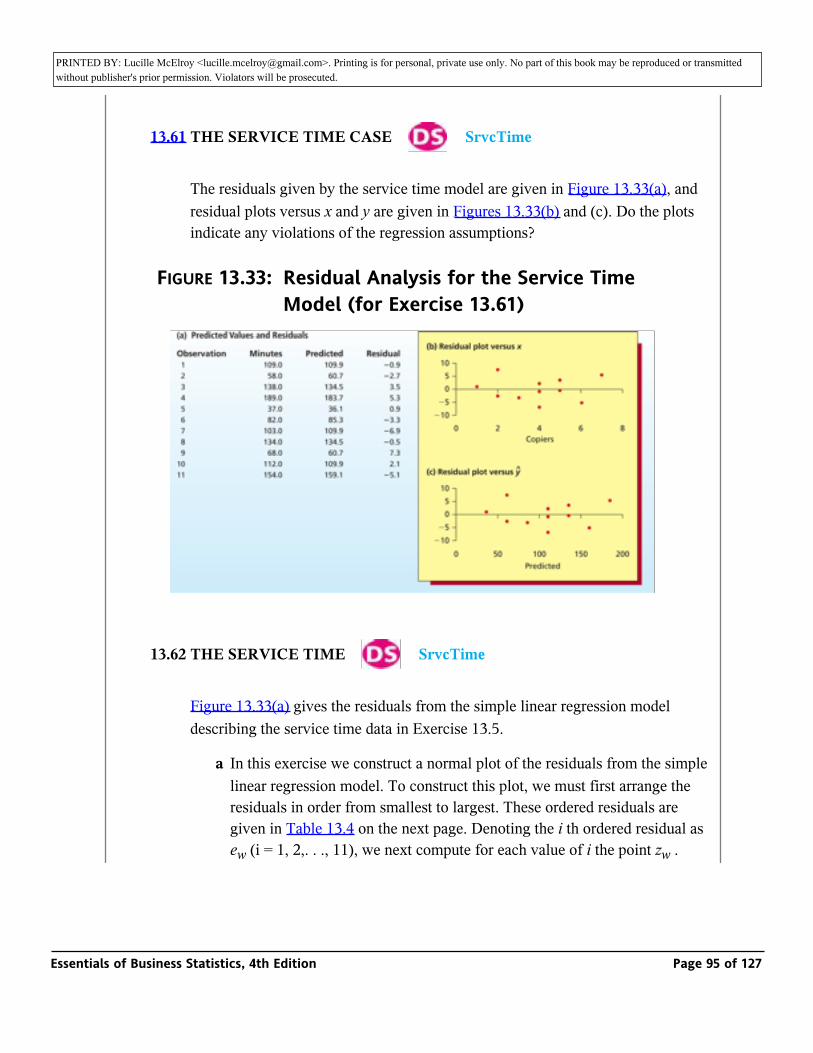
PRINTED BY: Lucille McElroy <[email protected]>. Printing is for personal, private use only. No part of this book may be reproduced or transmitted without publisher's prior permission. Violators will be prosecuted.violations of the regression assumptions.
13.61 THE SERVICE TIME CASE _ SrvcTime
The residuals given by the service time model are given in Figure 13.33(a), and residual plots versus x and y are given in Figures 13.33(b) and (c). Do the plots indicate any violations of the regression assumptions?
FIGURE 13.33: Residual Analysis for the Service Time Model (for Exercise 13.61)
13.62 THE SERVICE TIME _ SrvcTime
Figure 13.33(a) gives the residuals from the simple linear regression model describing the service time data in Exercise 13.5.
a In this exercise we construct a normal plot of the residuals from the simple linear regression model. To construct this plot, we must first arrange the residuals in order from smallest to largest. These ordered residuals are given in Table 13.4 on the next page. Denoting the i th ordered residual as ew (i = 1, 2,. . ., 11), we next compute for each value of i the point zw .
Essentials of Business Statistics, 4th Edition Page 95 of 127
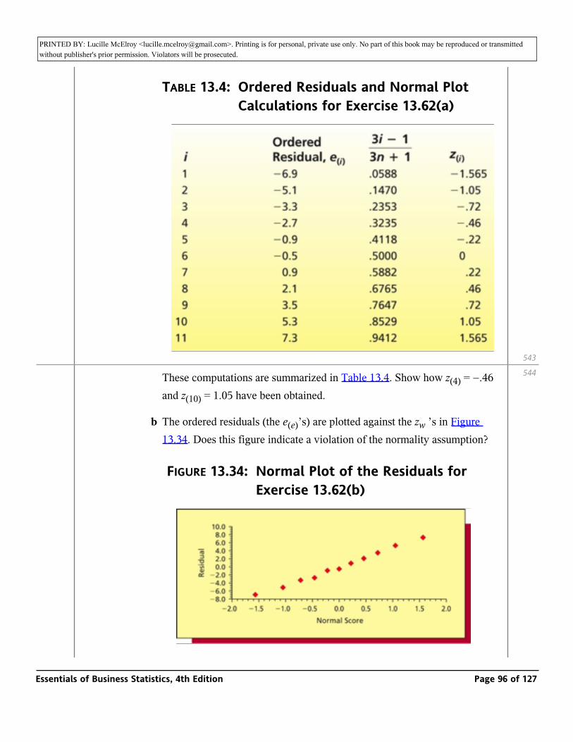
PRINTED BY: Lucille McElroy <[email protected]>. Printing is for personal, private use only. No part of this book may be reproduced or transmitted without publisher's prior permission. Violators will be prosecuted.ew (i = 1, 2,. . ., 11), we next compute for each value of i the point zw .
TABLE 13.4: Ordered Residuals and Normal Plot Calculations for Exercise 13.62(a)
These computations are summarized in Table 13.4. Show how z(4) = −.46 and z(10) = 1.05 have been obtained.
b The ordered residuals (the e(e)’s) are plotted against the zw ’s in Figure 13.34. Does this figure indicate a violation of the normality assumption?
FIGURE 13.34: Normal Plot of the Residuals for Exercise 13.62(b)
543
544
Essentials of Business Statistics, 4th Edition Page 96 of 127

PRINTED BY: Lucille McElroy <[email protected]>. Printing is for personal, private use only. No part of this book may be reproduced or transmitted without publisher's prior permission. Violators will be prosecuted.
13.63 A simple linear regression model is employed to analyze the 24 monthly observations given in Table 13.5. Residuals are computed and are plotted versus time. The resulting residual plot is shown in Figure 13.35. Discuss why the residual plot suggests the existence of positive autocorrelation. The Durbin–Watson statistic d can be calculated to be .473. Test for positive (first-order) autocorrelation at a = .05, and test for negative (first-order) autocorrelation at α
= .05 _ SalesAdv
TABLE 13.5: Sales and Advertising Data for
Exercise 13.63 _ SalesAdv
Essentials of Business Statistics, 4th Edition Page 97 of 127
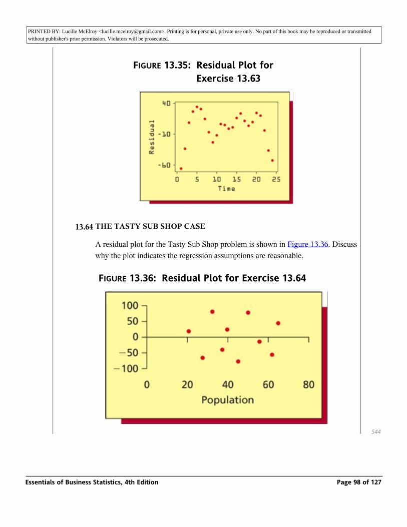
PRINTED BY: Lucille McElroy <[email protected]>. Printing is for personal, private use only. No part of this book may be reproduced or transmitted without publisher's prior permission. Violators will be prosecuted.
FIGURE 13.35: Residual Plot for Exercise 13.63
13.64 THE TASTY SUB SHOP CASE
A residual plot for the Tasty Sub Shop problem is shown in Figure 13.36. Discuss why the plot indicates the regression assumptions are reasonable.
FIGURE 13.36: Residual Plot for Exercise 13.64
544
Essentials of Business Statistics, 4th Edition Page 98 of 127

PRINTED BY: Lucille McElroy <[email protected]>. Printing is for personal, private use only. No part of this book may be reproduced or transmitted without publisher's prior permission. Violators will be prosecuted.
13.65 USING A NATURAL LOGARITHM TRANSFORMATION _
WestStk
Western Steakhouses, a fast-food chain, opened 15 years ago. Each year since then the number of steakhouses in operation, y, was recorded. An analyst for the firm wishes to use these data to predict the number of steakhouses that will be in operation next year. The data are given in the page margin, and a plot of the data is given in Figure 13.37(a). Examining the data plot, we see that the number of steakhouse openings has increased over time at an increasing rate and with increasing variation. A plot of the natural logarithms of the steakhouse values versus time (see Figure 13.37(b)) has a straight-line appearance with constant variation. Therefore, we consider the model ln yt = β0 + β1 t + εt . If we use MINITAB, we find that the least squares point estimates of β0 and β1 are β0 = 2.07012 and β1 = .256880. We also find that a point prediction of and a 95 percent prediction interval for the natural logarithm of the number of steakhouses in operation next year (year 16) are 6.1802 and [5.9945, 6.3659]. See the MINITAB output in Figure 13.38.
FIGURE 13.37: Data Plots for Exercise 13.65 DS WestStk
544
545
Essentials of Business Statistics, 4th Edition Page 99 of 127

PRINTED BY: Lucille McElroy <[email protected]>. Printing is for personal, private use only. No part of this book may be reproduced or transmitted without publisher's prior permission. Violators will be prosecuted.
FIGURE 13.38: MINITAB Output of a Regression Analysis of the Steakhouse Data Using the Model y * = µ0 + µ1 x + ε, where y * = ln y (for Exercise 13.65)
a Use the least squares point estimates to verify the point prediction.
b By exponentiating the point prediction and prediction interval—that is, by calculating e 61802 and [e 5.9945, e 6.3659 ]—find a point prediction of and a 95 percent prediction interval for the number of steakhouses in operation next year.
c The model ln yt = β0 + β1 t + εt is called a growth curve model because it implies that
where α0 = e β0, α1 = e β1 and ηt = eεt. Here α1 = eβl is called the growth rate of the y values. Noting that the least squares point estimate of β1 is µ1 = .256880, estimate the growth rate α1. Also, interpret this growth rate by using the fact that
yt = α0 α1t ηt = (α0 α1t-1)α1 ηt ≠ (yt-1)α1 ηt. This says that yt is expected to be approximately α1 times yt-1.
Essentials of Business Statistics, 4th Edition Page 100 of 127

PRINTED BY: Lucille McElroy <[email protected]>. Printing is for personal, private use only. No part of this book may be reproduced or transmitted without publisher's prior permission. Violators will be prosecuted.approximately α1 times yt-1.
The Steakhouse Data
545
Essentials of Business Statistics, 4th Edition Page 101 of 127

PRINTED BY: Lucille McElroy <[email protected]>. Printing is for personal, private use only. No part of this book may be reproduced or transmitted without publisher's prior permission. Violators will be prosecuted.
13.10: Some Shortcut Formulas (Optional)
Calculating the sum of squared residuals
A shortcut formula for the sum of squared residuals is
where
For example, consider the Tasty Sub Shop case. If we square each of the ten observed yearly revenues in Table 13.1 (page 492) and add up the resulting squared values, we find that ∑yi
2 = 7,897,109.47. We have also found in Example 13.2 (page 497) that ∑yi = 8603.1, SSxy = 29,836.389 and SSxx = 1,913.129. It follows that
and
545
546
546
547
1...
13.1...
Essentials of Business Statistics, 4th Edition Page 102 of 127

PRINTED BY: Lucille McElroy <[email protected]>. Printing is for personal, private use only. No part of this book may be reproduced or transmitted without publisher's prior permission. Violators will be prosecuted.
Finally, note that SS2xy /SSxx equals b1SSxy. However, we recommend using the first of these
expressions, because doing so usually gives less round-off error.
Calculating the total, explained, and unexplained variations
The unexplained variation is SSE, and thus the shortcut formula for SSE is a shortcut formula for the unexplained variation. The quantity SSyy defined on page 546 is the total variation, and thus the shortcut formula for SSyy is a shortcut formula for the total variation. Lastly, it can be shown that the expression SS 2 xy /SSxx equals the explained variation and thus is a shortcut formula for this quantity.
Chapter Summary
This chapter has discussed simple linear regression analysis, which relates a dependent variable to a single independent (predictor) variable. We began by considering the simple linear regression model, which employs two parameters: the slope and y intercept. We next discussed how to compute the least squares point estimates of these parameters and how to use these estimates to calculate a point estimate of the mean value of the dependent variable and a point prediction of an individual value of the dependent variable. Then, after considering the assumptions behind the simple linear regression model, we discussed testing the significance of the regression relationship (slope), calculating a confidence interval for the mean value of the dependent variable, and calculating a prediction interval for an individual value of the dependent variable. We next explained several measures of the utility of the simple linear regression model. These include the simple coefficient of determination and an F test for the simple linear model. We concluded this chapter by giving a discussion of using residual analysis to detect violations of the regression assumptions. We learned that we can sometimes remedy violations of these assumptions by transforming the dependent variable.
Glossary of Terms
dependent variable:
The variable that is being described, predicted, or controlled. (page 491)
distance value:
A measure of the distance between a particular value x0 of the independent variable x and, the average of the previously observed values of x (the center of the experimental region). (page 515)
13.1...
1...
1...
Essentials of Business Statistics, 4th Edition Page 103 of 127

PRINTED BY: Lucille McElroy <[email protected]>. Printing is for personal, private use only. No part of this book may be reproduced or transmitted without publisher's prior permission. Violators will be prosecuted.
error term:
The difference between an individual value of the dependent variable and the corresponding mean value of the dependent variable. (page 494)
experimental region:
The range of the previously observed values of the independent variable. (page 498)
independent variable:
A variable used to describe, predict, and control the dependent variable. (page 491)
least squares point estimates:
The point estimates of the slope and y intercept of the simple linear regression model that minimize the sum of squared residuals. (pages 496–497)
negative autocorrelation:
The situation in which positive error terms tend to be followed over time by negative error terms and negative error terms tend to be followed over time by positive error terms. (page 536)
normal plot:
A residual plot that is used to check the normality assumption. (page 534)
positive autocorrelation:
The situation in which positive error terms tend to be followed over time by positive error terms and x negative error terms tend to be followed over time by negative error terms. (page 535)
residual:
The difference between the observed value of the dependent variable and the corresponding predicted value of the dependent variable. (pages 496, 531)
Essentials of Business Statistics, 4th Edition Page 104 of 127

PRINTED BY: Lucille McElroy <[email protected]>. Printing is for personal, private use only. No part of this book may be reproduced or transmitted without publisher's prior permission. Violators will be prosecuted.
residual plot:
A plot of the residuals against some criterion. The plot is used to check the validity of one or more regression assumptions. (page 531)
simple coefficient of determination:
The proportion of the total variation in the observed values of the dependent variable that is explained by the simple linear regression model. (page 522)
simple correlation coefficient:
A measure of the linear association between two variables. (page 523)
simple linear regression model:
An equation that describes the straight-line relationship between a dependent variable and an independent variable. (page 494)
slope (of the simple linear regression model):
The change in the mean value of the dependent variable that is associated with a one-unit increase in the value of the independent variable. (page 494)
y -intercept (of the simple linear regression model):
The mean value of the dependent variable when the value of the independent variable is 0. (page 494)
Important Formulas and Tests
Simple linear regression model: page 494
Least squares point estimates of b0 and b1 : page 496
Least squares line (prediction equation): page 496
547
5481...
Essentials of Business Statistics, 4th Edition Page 105 of 127
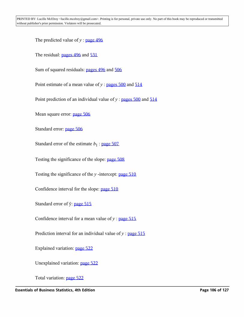
PRINTED BY: Lucille McElroy <[email protected]>. Printing is for personal, private use only. No part of this book may be reproduced or transmitted without publisher's prior permission. Violators will be prosecuted.Least squares line (prediction equation): page 496
The predicted value of y : page 496
The residual: pages 496 and 531
Sum of squared residuals: pages 496 and 506
Point estimate of a mean value of y : pages 500 and 514
Point prediction of an individual value of y : pages 500 and 514
Mean square error: page 506
Standard error: page 506
Standard error of the estimate b1 : page 507
Testing the significance of the slope: page 508
Testing the significance of the y -intercept: page 510
Confidence interval for the slope: page 510
Standard error of ŷ: page 515
Confidence interval for a mean value of y : page 515
Prediction interval for an individual value of y : page 515
Explained variation: page 522
Unexplained variation: page 522
Total variation: page 522
Essentials of Business Statistics, 4th Edition Page 106 of 127
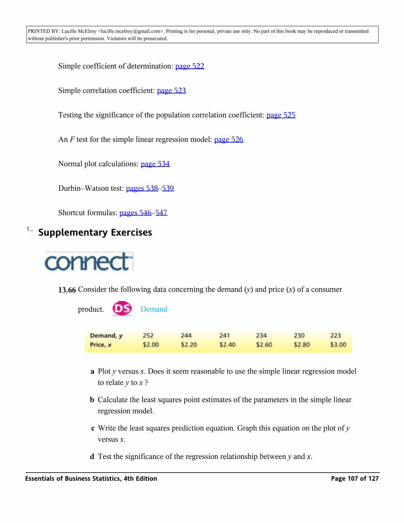
PRINTED BY: Lucille McElroy <[email protected]>. Printing is for personal, private use only. No part of this book may be reproduced or transmitted without publisher's prior permission. Violators will be prosecuted.Total variation: page 522
Simple coefficient of determination: page 522
Simple correlation coefficient: page 523
Testing the significance of the population correlation coefficient: page 525
An F test for the simple linear regression model: page 526
Normal plot calculations: page 534
Durbin–Watson test: pages 538–539
Shortcut formulas: pages 546–547
Supplementary Exercises
_
13.66 Consider the following data concerning the demand (y) and price (x) of a consumer
product. _ Demand
a Plot y versus x. Does it seem reasonable to use the simple linear regression model to relate y to x ?
b Calculate the least squares point estimates of the parameters in the simple linear regression model.
c Write the least squares prediction equation. Graph this equation on the plot of y versus x.
d Test the significance of the regression relationship between y and x.
1...
Essentials of Business Statistics, 4th Edition Page 107 of 127

PRINTED BY: Lucille McElroy <[email protected]>. Printing is for personal, private use only. No part of this book may be reproduced or transmitted without publisher's prior permission. Violators will be prosecuted.d Test the significance of the regression relationship between y and x.
e Find a point prediction of and a 95 percent prediction interval for the demand corresponding to each of the prices $2.10, $2.75, and $3.10.
13.67 In an article in Public Roads (1983), Bissell, Pilkington, Mason, and Woods study bridge safety (measured in accident rates per 100 million vehicles) and the difference between the width of the bridge and the width of the roadway approach (road plus shoulder):4 AutoAcc
The MINITAB output of a simple linear regression analysis relating accident to width difference is as follows:
Using the MINITAB output
a Identify and interpret the least squares point estimate of the slope of the simple linear regression model.
b Identify and interpret the p -value for testing H0 : β1 0 versus Ha : β1 ≠ 0.
c Identify and interpret r 2.
13.68 The data in Table 13.6 concerning the relationship between smoking and lung cancer death are presented in a course of The Open University, Statistics in Society, Unit C4, The Open University Press, Milton Keynes, England, 1983. The original source of the data is Occupational Mortality: The Registrar General’s Decennial Supplement for England and Wales, 1970–1972, Her Majesty’s Stationery Office, London, 1978. In the table, a smoking index greater (less) than 100 indicates that men in the occupational group smoke more (less) than average when compared to all men of the same age.
548
549
Essentials of Business Statistics, 4th Edition Page 108 of 127

PRINTED BY: Lucille McElroy <[email protected]>. Printing is for personal, private use only. No part of this book may be reproduced or transmitted without publisher's prior permission. Violators will be prosecuted.table, a smoking index greater (less) than 100 indicates that men in the occupational
group smoke more (less) than average when compared to all men of the same age. Similarly, a lung cancer death index greater (less) than 100 indicates that men in the occupational group have a greater (less) than average lung cancer death rate when compared to all men of the same age. In Figure 13.39 we present a portion of a MINITAB output of a simple linear regression analysis relating the lung cancer death index to the smoking index. In Figure 13.40 we present a plot of the lung cancer death
index versus the smoking index. _ Smoking
TABLE 13.6: The Smoking and Lung Cancer Death Data
_ Smoking
FIGURE 13.39: MINITAB Output of a Simple Linear Regression Analysis of the Data in Table 13.6
Essentials of Business Statistics, 4th Edition Page 109 of 127
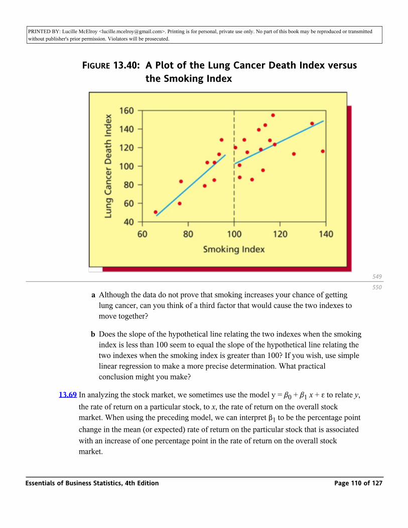
PRINTED BY: Lucille McElroy <[email protected]>. Printing is for personal, private use only. No part of this book may be reproduced or transmitted without publisher's prior permission. Violators will be prosecuted.
FIGURE 13.40: A Plot of the Lung Cancer Death Index versus the Smoking Index
a Although the data do not prove that smoking increases your chance of getting lung cancer, can you think of a third factor that would cause the two indexes to move together?
b Does the slope of the hypothetical line relating the two indexes when the smoking index is less than 100 seem to equal the slope of the hypothetical line relating the two indexes when the smoking index is greater than 100? If you wish, use simple linear regression to make a more precise determination. What practical conclusion might you make?
13.69 In analyzing the stock market, we sometimes use the model y = β0 + β1 x + ε to relate y, the rate of return on a particular stock, to x, the rate of return on the overall stock market. When using the preceding model, we can interpret β1 to be the percentage point change in the mean (or expected) rate of return on the particular stock that is associated with an increase of one percentage point in the rate of return on the overall stock market.
549
550
Essentials of Business Statistics, 4th Edition Page 110 of 127

PRINTED BY: Lucille McElroy <[email protected]>. Printing is for personal, private use only. No part of this book may be reproduced or transmitted without publisher's prior permission. Violators will be prosecuted.market.
If regression analysis can be used to conclude (at a high level of confidence) that β1 is greater than 1 (for example, if the 95 percent confidence interval for β1 were [1.1826, 1.4723]), this indicates that the mean rate of return on the particular stock changes more quickly than the rate of return on the overall stock market. Such a stock is called an aggressive stock because gains for such a stock tend to be greater than overall market gains (which occur when the market is bullish). However, losses for such a stock tend to be greater than overall market losses (which occur when the market is bearish). Aggressive stocks should be purchased if you expect the market to rise and avoided if you expect the market to fall.
If regression analysis can be used to conclude (at a high level of confidence) that b1 is less than 1 (for example, if the 95 percent confidence interval for β1 were [.4729, .7861]), this indicates that the mean rate of return on the particular stock changes more slowly than the rate of return on the overall stock market. Such a stock is called a defensive stock. Losses for such a stock tend to be less than overall market losses, whereas gains for such a stock tend to be less than overall market gains. Defensive stocks should be held if you expect the market to fall and sold off if you expect the market to rise.
If the least squares point estimate b1 of b1 is nearly equal to 1, and if the 95 percent confidence interval for b1 contains 1, this might indicate that the mean rate of return on the particular stock changes at roughly the same rate as the rate of return on the overall stock market. Such a stock is called a neutral stock.
In a 1984 article in Financial Analysts Journal, Haim Levy considers how a stock’s value of β1 depends on the length of time for which the rate of return is calculated. Levy calculated estimated values of β1 for return length times varying from 1 to 30 months for each of 38 aggressive stocks, 38 defensive stocks, and 68 neutral stocks. Each estimated value was based on data from 1946 to 1975. In Table 13.7 we present the average estimate of β1 for each stock type for different return length times. Let y = average estimate of β1 and x = return length time, and consider relating y to x for each
stock type by using the simple linear regression model y = β0 * + β1 * x + ε Here β0 *
and β1 * are regression parameters relating y to x. We use the asterisks to indicate that these regression parameters are different from β0 and β1. Calculate a 95 percent
confidence interval for β1 * for each stock type. Carefully interpret the meaning of each interval.
550
551
Essentials of Business Statistics, 4th Edition Page 111 of 127

PRINTED BY: Lucille McElroy <[email protected]>. Printing is for personal, private use only. No part of this book may be reproduced or transmitted without publisher's prior permission. Violators will be prosecuted.interval.
TABLE 13.7: Return Length Estimates ofβ1
13.70 On January 28, 1986, the space shuttle Challenger exploded soon after takeoff, killing all eight astronauts aboard. The temperature at the Kennedy Space Center at liftoff was 31°F. Before the launch, several scientists argued that the launch should be delayed because the shuttle’s O-rings might harden in the cold and leak. Other scientists used the data plot in Figure 13.41 to argue that there was no relationship between temperature and O-ring failure. On the basis of this figure and other considerations, Challenger was launched to its disastrous, last flight.
Essentials of Business Statistics, 4th Edition Page 112 of 127

PRINTED BY: Lucille McElroy <[email protected]>. Printing is for personal, private use only. No part of this book may be reproduced or transmitted without publisher's prior permission. Violators will be prosecuted.Challenger was launched to its disastrous, last flight.
FIGURE 13.41: A Data Plot Based on Seven Launches
Scientists using the data plot in Figure 13.41 made a horrible mistake. They relied on a data plot that was created by using only the seven previous launches where there was at least one O-ring failure. A plot based on all 24 previous launches—17 of which had no O-ring failures—is given in Figure 13.42.
FIGURE 13.42: A Data Plot Based on All 24 Launches
Essentials of Business Statistics, 4th Edition Page 113 of 127
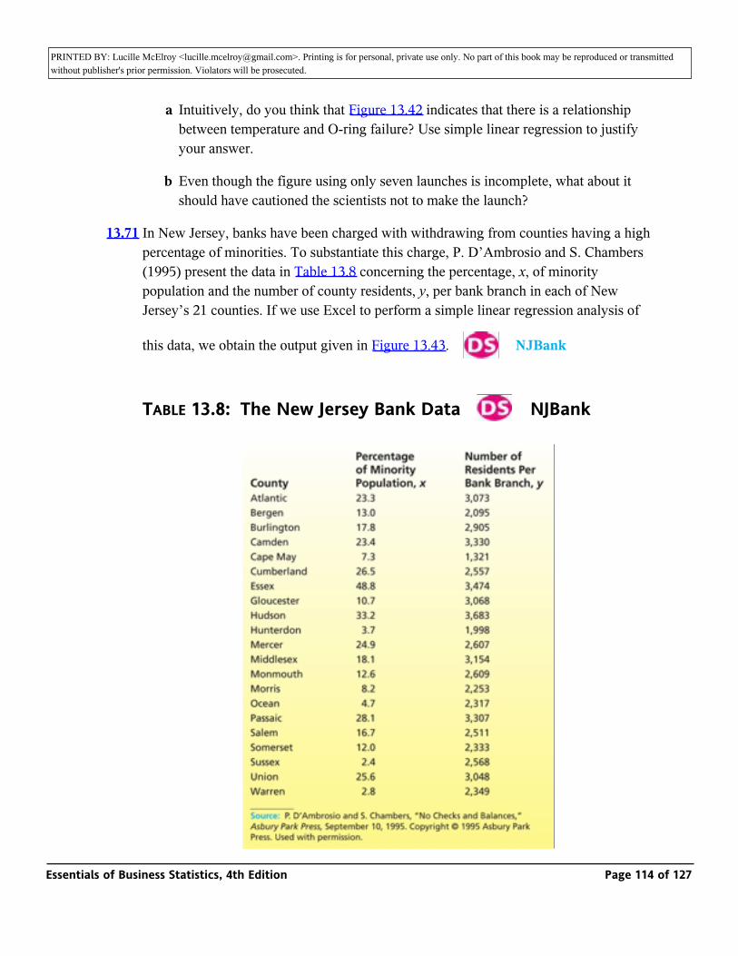
PRINTED BY: Lucille McElroy <[email protected]>. Printing is for personal, private use only. No part of this book may be reproduced or transmitted without publisher's prior permission. Violators will be prosecuted.
a Intuitively, do you think that Figure 13.42 indicates that there is a relationship between temperature and O-ring failure? Use simple linear regression to justify your answer.
b Even though the figure using only seven launches is incomplete, what about it should have cautioned the scientists not to make the launch?
13.71 In New Jersey, banks have been charged with withdrawing from counties having a high percentage of minorities. To substantiate this charge, P. D’Ambrosio and S. Chambers (1995) present the data in Table 13.8 concerning the percentage, x, of minority population and the number of county residents, y, per bank branch in each of New Jersey’s 21 counties. If we use Excel to perform a simple linear regression analysis of
this data, we obtain the output given in Figure 13.43. _ NJBank
TABLE 13.8: The New Jersey Bank Data _ NJBank
Essentials of Business Statistics, 4th Edition Page 114 of 127

PRINTED BY: Lucille McElroy <[email protected]>. Printing is for personal, private use only. No part of this book may be reproduced or transmitted without publisher's prior permission. Violators will be prosecuted.
FIGURE 13.43: Excel Output of a Simple Linear Regression Analysis of the New Jersey Bank Data
a Determine if there is a significant relationship between x and y.
b Describe the exact nature of any relationship that exists between x and y. (Hint: Estimate β1 by a point estimate and a confidence interval.)
Note: The Internet exercise for this chapter is on page 557.
Appendix 13.1: _ Simple Linear Regression Analysis Using Excel
The instruction blocks in this section each begins by describing the entry of data into an Excel spreadsheet. Alternatively, the data may be loaded directly from the data disk included with the text. The appropriate data file name is given at the top of each instruction block. Please refer to Appendix 1.1 for further information about entering data, saving data, and printing results when using Excel.
Simple linear regression in Figure 13.9 on page 511 (data file: FuelCon1.xlsx):
• Enter the fuel consumption data (page 501)—the temperatures in column A with label Temp and the fuel consumptions in column B with label FuelCons.
• Select Data : Data Analysis : Regression and click OK in the Data Analysis dialog box.
• In the Regression dialog box: Enter B1:B9 into the “Input Y Range” box. Enter A1:A9 into the “Input X Range” box.
• Place a checkmark in the Labels checkbox.
• Be sure that the “Constant is Zero” checkbox is NOT checked.
551
552
1...
Essentials of Business Statistics, 4th Edition Page 115 of 127

PRINTED BY: Lucille McElroy <[email protected]>. Printing is for personal, private use only. No part of this book may be reproduced or transmitted without publisher's prior permission. Violators will be prosecuted.• Be sure that the “Constant is Zero” checkbox is NOT checked.
• Select the “New Worksheet Ply” option.
• Click OK in the Regression dialog box to obtain the regression results in a new worksheet.
Essentials of Business Statistics, 4th Edition Page 116 of 127
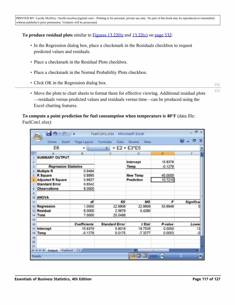
PRINTED BY: Lucille McElroy <[email protected]>. Printing is for personal, private use only. No part of this book may be reproduced or transmitted without publisher's prior permission. Violators will be prosecuted.
To produce residual plots similar to Figures 13.22(b) and 13.22(c) on page 532:
• In the Regression dialog box, place a checkmark in the Residuals checkbox to request predicted values and residuals.
• Place a checkmark in the Residual Plots checkbox.
• Place a checkmark in the Normal Probability Plots checkbox.
• Click OK in the Regression dialog box.
• Move the plots to chart sheets to format them for effective viewing. Additional residual plots—residuals versus predicted values and residuals versus time—can be produced using the Excel charting features.
To compute a point prediction for fuel consumption when temperature is 40°F (data file: FuelCon1.xlsx):
552
553
Essentials of Business Statistics, 4th Edition Page 117 of 127

PRINTED BY: Lucille McElroy <[email protected]>. Printing is for personal, private use only. No part of this book may be reproduced or transmitted without publisher's prior permission. Violators will be prosecuted.
• The Excel Analysis ToolPak does not provide an option for computing point or interval predictions. A point prediction can be computed from the regression results using Excel cell formulas.
• In the regression output, the estimated intercept and slope parameters from cells A17:B18 have been copied to cells D2:E3 and the predictor value 40 has been placed in cell E5.
• In cell E6, enter the Excel formula = E2 + E3*E5 (= 10.7210) to compute the prediction.
Simple linear regression with a transformed response similar to Figure 13.30 on page 541 (data file: QHIC.xlsx):
• Enter the QHIC upkeep expenditure data from Figure 13.21 (page 530). Enter the label Value in cell A1 with the home values in cells A2 to A41 and enter the label Upkeep in cell B1 with the upkeep expenditures in cells B2 to B41.
• Enter the label SqUpkeep in cell C1.
• Click on cell C2 and then select the Insert Function button _ on the Excel ribbon.
• Select Math & Trig from the “Or select a category:” menu, select SQRT from the “Select a function:” menu, and click OK in the Insert Function dialog box.
• In the “SQRT Function Arguments” dialog box, enter B2 in the Number box and click OK to compute the square root of the value in B2.
• Copy the cell formula of C2 through cell C41 by double-clicking the drag handle (in the lower right corner) of cell C2 to compute the square roots of the remaining upkeep values.
• Follow the steps for simple linear regression (on page 552) using cells C1:C41 as the response (Input Y Range) and cells A1:A41 as the predictor (Input X Range).
Essentials of Business Statistics, 4th Edition Page 118 of 127

PRINTED BY: Lucille McElroy <[email protected]>. Printing is for personal, private use only. No part of this book may be reproduced or transmitted without publisher's prior permission. Violators will be prosecuted.response (Input Y Range) and cells A1:A41 as the predictor (Input X Range).
553Essentials of Business Statistics, 4th Edition Page 119 of 127
PRINTED BY: Lucille McElroy <[email protected]>. Printing is for personal, private use only. No part of this book may be reproduced or transmitted without publisher's prior permission. Violators will be prosecuted.
Appendix 13.2: _ Simple Linear Regression Analysis Using
MegaStat
The instructions in this section begin by describing the entry of data into an Excel worksheet. Alternatively, the data may be downloaded from this book’s website. The appropriate data file name is given at the top of each instruction block. Please refer to Appendix 1.1 for further information about entering data, saving data, and printing results in Excel. Please refer to Appendix 1.2 for more information about using MegaStat.
Simple linear regression for the service time data in Exercise 13.5 on page 501 (data file: SrvcTime.xlsx):
• Enter the service time data (page 502) with the numbers of copiers serviced in column A with label Copiers and with the service times in column B with label Minutes.
• Select Add-Ins : MegaStat : Correlation/Regression : Regression Analysis.
• In the Regression Analysis dialog box, click in the Independent Variables window and use the autoexpand feature to enter the range A1 : A12.
• Click in the Dependent Variable window and use the autoexpand feature to enter the range B1 : B12.
• Check the appropriate Options and Residuals checkboxes as follows:
1 Check “Test Intercept” to include a y -intercept and to test its significance.
2 Check “Output Residuals” to obtain a list of the model residuals.
3 Check “Plot Residuals by Observation,” and “Plot Residuals by Predicted Y and X” to obtain residual plots versus time, versus the predicted values of y, and versus the values of the independent variable.
4 Check “Normal Probability Plot of Residuals” to obtain a normal plot.
5 Check “Durbin-Watson” for the Durbin–Watson statistic.
To obtain a point prediction of y when four computers will be serviced (as well as a confidence interval and prediction interval):
• Click on the drop-down menu above the Predictor Values window and select “Type in predictor values.”
553
5541...
Essentials of Business Statistics, 4th Edition Page 120 of 127

PRINTED BY: Lucille McElroy <[email protected]>. Printing is for personal, private use only. No part of this book may be reproduced or transmitted without publisher's prior permission. Violators will be prosecuted.predictor values.”
• Type the value of the independent variable for which a prediction is desired (here equal to 4) into the Predictor Values window.
• Select a desired level of confidence (here 95%) from the Confidence Level drop-down menu or type in a value.
• Click OK in the Regression Analysis dialog box.
554Essentials of Business Statistics, 4th Edition Page 121 of 127
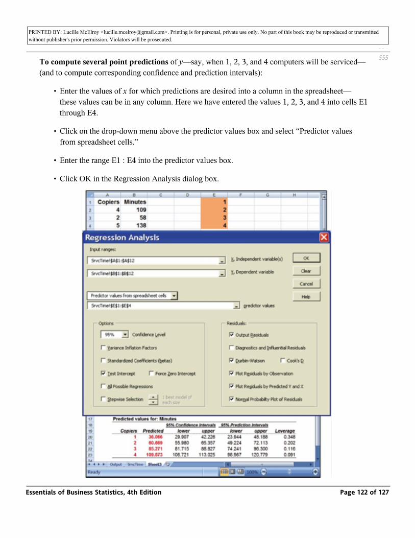
PRINTED BY: Lucille McElroy <[email protected]>. Printing is for personal, private use only. No part of this book may be reproduced or transmitted without publisher's prior permission. Violators will be prosecuted.
To compute several point predictions of y—say, when 1, 2, 3, and 4 computers will be serviced—(and to compute corresponding confidence and prediction intervals):
• Enter the values of x for which predictions are desired into a column in the spreadsheet—these values can be in any column. Here we have entered the values 1, 2, 3, and 4 into cells E1 through E4.
• Click on the drop-down menu above the predictor values box and select “Predictor values from spreadsheet cells.”
• Enter the range E1 : E4 into the predictor values box.
• Click OK in the Regression Analysis dialog box.
554
555
Essentials of Business Statistics, 4th Edition Page 122 of 127

PRINTED BY: Lucille McElroy <[email protected]>. Printing is for personal, private use only. No part of this book may be reproduced or transmitted without publisher's prior permission. Violators will be prosecuted.
Simple linear regression with a transformed response similar to Figure 13.30 on page 541 (data file: QHIC.xlsx):
• Enter the QHIC data from Figure 13.21 (page 530)—the home values in column A (with label Value) and the upkeep expenditures in column B (with label Upkeep).
• Follow the instructions on page 553 in Appendix 13.1 to calculate the square roots of the upkeep expenditures in column C (with label SRUpkeep).
• Select Add-Ins : MegaStat : Correlation/Regression : Regression Analysis.
• In the Regression Analysis dialog box, click in the Independent variables window, and use the AutoExpand feature to enter the range A1 : A41.
• Click in the Dependent variable window and use the AutoExpand feature to enter the range C1 : C41.
• Check the “Test Intercept” checkbox to include a y -intercept and test its significance.
Essentials of Business Statistics, 4th Edition Page 123 of 127

PRINTED BY: Lucille McElroy <[email protected]>. Printing is for personal, private use only. No part of this book may be reproduced or transmitted without publisher's prior permission. Violators will be prosecuted.
To compute a point prediction of the square root of y (as well as a confidence interval and prediction interval) for a house having a value of $220,000:
• Select “Type in predictor values” from the drop-down menu above the predictor values window.
• Type 220 into the predictor values window.
• Select a desired level of confidence (here 95%) from the drop-down menu in the Confidence Level box or type in a value.
• Click OK in the Regression Analysis dialog box.
Appendix 13.3: _ Simple Linear Regression Analysis Using
MINITAB
The instruction blocks in this section each begins by describing the entry of data into the MINITAB data window. Alternatively, the data may be downloaded from this book’s website. The appropriate data file name is given at the top of each instruction block. Please refer to Appendix 1.3 for further information about entering data, saving data, and printing results when using MINITAB.
Simple linear regression of the fuel consumption data in Figure 13.10 on page 511 (data file: FuelCon1. MTW):
555
556
556
1...
Essentials of Business Statistics, 4th Edition Page 124 of 127
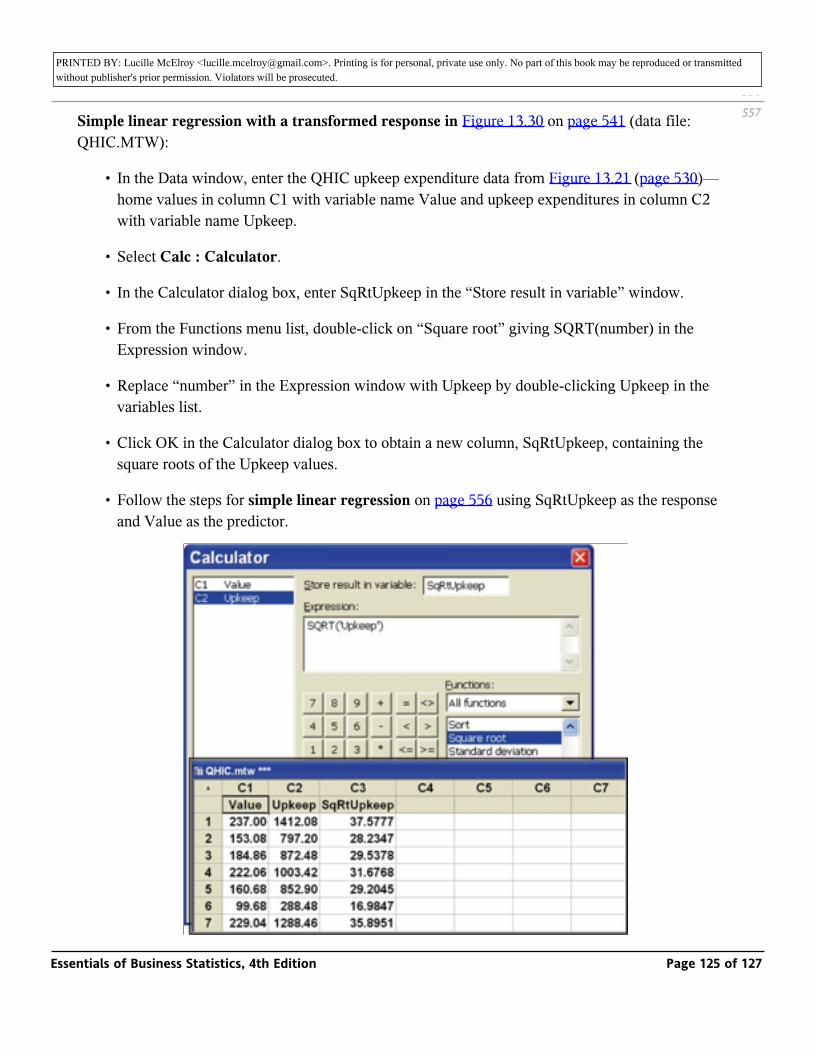
PRINTED BY: Lucille McElroy <[email protected]>. Printing is for personal, private use only. No part of this book may be reproduced or transmitted without publisher's prior permission. Violators will be prosecuted.
Simple linear regression with a transformed response in Figure 13.30 on page 541 (data file: QHIC.MTW):
• In the Data window, enter the QHIC upkeep expenditure data from Figure 13.21 (page 530)—home values in column C1 with variable name Value and upkeep expenditures in column C2 with variable name Upkeep.
• Select Calc : Calculator.
• In the Calculator dialog box, enter SqRtUpkeep in the “Store result in variable” window.
• From the Functions menu list, double-click on “Square root” giving SQRT(number) in the Expression window.
• Replace “number” in the Expression window with Upkeep by double-clicking Upkeep in the variables list.
• Click OK in the Calculator dialog box to obtain a new column, SqRtUpkeep, containing the square roots of the Upkeep values.
• Follow the steps for simple linear regression on page 556 using SqRtUpkeep as the response and Value as the predictor.
556
557
Essentials of Business Statistics, 4th Edition Page 125 of 127

PRINTED BY: Lucille McElroy <[email protected]>. Printing is for personal, private use only. No part of this book may be reproduced or transmitted without publisher's prior permission. Violators will be prosecuted.
13.72: Internet Exercise
The U.S. News & World Report website provides rankings of the best colleges and universities in the United States. The free version of Best Colleges gives information such as number of students enrolled, tuition rates, and so forth. Among the data provided are the percentage acceptance rate (at the time of this writing the data are for the fall semester of 2008) and the average freshman retention rate (at the time of this writing, the average percentage of freshman entering starting in 2005 through 2008 who returned to school the following fall is given).
One might wonder if there is a statistically significant relationship between average freshman percentage retention rate and the percentage acceptance rate at colleges and universities in the United States. To investigate this possible relationship, go to the U.S. News & World Report website (www.usnews.com). Then make selections as follows: Education; Best Colleges; National Universities; View National Universities Rankings. From the rankings, randomly select a list of the ranked universities and their most recent acceptance rates. Note that following the list of ranked universities is a list of unranked schools. Omit these unranked schools from your analysis. Next, return to the National Universities page and select Freshman Retention Rate from the National Universities Quick Comparison list. Compile a list of average retention rates for the schools in your list of ranked universities. Finally, enter the ranked universities and their corresponding acceptance rates and average freshman retention rates into a spreadsheet.
Using Excel or MINITAB, construct a scatter plot of average freshman retention rate versus acceptance rate. Describe any apparent relationship between these variables. Develop a simple linear regression model expressing average freshman retention rate as a linear function of acceptance rate. Then use Excel or MINITAB to fit the model. Using the computer output, identify the key summary measures—r 2, the standard error, and the F -statistic from the ANOVA table. Identify and interpret the estimated regression coefficients. Suppose that a university has an acceptance rate of 90 percent. Use your regression model to predict the average freshman retention rate for this school. Prepare a brief report summarizing your analysis and conclusions.
1 www.quiznosfranchises.com/top-food-franchise-faqs.
2 In order to simplify notation, we will often drop the limits on summations in this and subsequent chapters. That is,
instead of using the summation _ .we will simply write ΣΣi = 1
n
3 Essentially, the difference between r and b1 is a change of scale. It can be shown that b1 and r are related by the
equatio b = (ssyy /ssxx)1/2 r .
13.1...
Essentials of Business Statistics, 4th Edition Page 126 of 127

PRINTED BY: Lucille McElroy <[email protected]>. Printing is for personal, private use only. No part of this book may be reproduced or transmitted without publisher's prior permission. Violators will be prosecuted.
4 Source: H. H. Bissell, G. B. Pilkington II, J. M. Mason, and D. L. Woods, “Roadway Cross Section and Alignment,” Public Roads 46 (March 1983), pp. 132–41.
Essentials of Business Statistics, 4th Edition Page 127 of 127